https://doi.org/10.1007/s00348-018-2518-z
RESEARCH ARTICLE
Experiments on a smooth wall hypersonic boundary layer at Mach 6
Dominik Neeb1 · Dominik Saile1 · Ali Gülhan1Received: 21 August 2017 / Revised: 3 February 2018 / Accepted: 15 February 2018 © The Author(s) 2018
Abstract
The turbulent boundary layer along the surface of high-speed vehicles drives shear stress and heat flux. Although essential to the vehicle design, the understanding of compressible turbulent boundary layers at high Mach numbers is limited due to the lack of available data. This is particularly true if the surface is rough, which is typically the case for all technical surfaces. To validate a methodological approach, as initial step, smooth wall experiments were performed. A hypersonic turbulent boundary layer at Ma = 6 ( Mae=5.4 ) along a 7◦ sharp cone model at low Reynolds numbers Re𝜃≈3000 was characterized.
The mean velocities in the boundary layer were acquired by means of Pitot pressure and particle image velocimetry (PIV) measurements. Furthermore, the PIV data were used to extract turbulent intensities along the profile. The mean velocities in the boundary layer agree with numerical data, independent of the measurement technique. Based on the profile data, three dif-ferent approaches to extract the skin friction velocity were applied and show favorable comparison to literature and numerical data. The extracted values were used for inner and outer scaling of the van Driest transformed velocity profiles which are in good agreement to incompressible theoretical data. Morkovin scaled turbulent intensities show ambiguous results compared to literature data which may be influenced by inflow turbulence level, particle lag and other measurement uncertainties.
1 Introduction
The thin flow region close to the surface of high-speed vehi-cles, dominated by the boundary layer, drives shear stress and heat flux. Therefore this region essentially influences the vehicle design, including components like aerothermal protection systems. This is in particular true if the boundary layer is turbulent, which is connected to increased gradients in the flow and therefore increased shear and heat flux. The understanding of compressible turbulent boundary layers at high Mach numbers is limited due to the lack of available data. This is especially true if additional aspects like sur-face roughness influence the flow. For the spacecraft design, this typically results in large safety margins which mean an increase in weight and cost. Therefore, further experi-mental data are important for the physical understanding and validation of state-of-the-art computations. However, accurate measurements of the compressible turbulent bound-ary layer in ground-based facilities is very challenging due
to a multitude of reasons, e.g., limited model dimensions, thin boundary layers, limited useable test times and inflow effects, like turbulence intensity. The choice of measurement technique is also a crucial parameter with high impact on spatial and temporal resolution.
At high speeds, density gradients influence the properties of the compressible boundary layer. Viscous heating within the boundary layer, which is caused by the deceleration of the fluid, is responsible for high-density gradients. But also the wall temperature affects the near wall density. This com-plicates the definition of driving parameters for the flow, like the Reynolds number. For incompressible flow, typically quantities of the free-stream or boundary layer edge condi-tions like density 𝜌
e , velocity ue and viscosity 𝜇e are
com-bined with a characteristic boundary layer length scale, such as the momentum loss thickness 𝜃 , to Re𝜃=𝜌eue𝜃∕𝜇e . Due
to the changing density in the compressible boundary layer, this definition might not be sufficient to capture, e.g., wall effects. This led to the definition of Re𝛿2=𝜌eue𝜃∕𝜇w , where the viscosity is defined at the wall, instead of the boundary layer edge, according to, e.g., Fernholz and Finley (1980), Duan and Martin (2011), Duan et al. (2011).
One attempt to study compressible boundary layers is to enable comparison to the larger database of the incompress-ible counterpart. This is done by accounting for the density
* Dominik Neeb
1 Institute of Aerodynamics and Flow Technology, Supersonic
and Hypersonic Technologies Department, German Aerospace Center (DLR), Cologne, Germany
gradient with specific scalings or transformations. A promi-nent and widely applied transformation for the mean velocity is the van Driest scaling (Van Driest 1951, 1956). It shows good results in a broad Mach number range at a variety of experimental (e.g., Humble et al. 2007; Ekoto et al. 2008; Sahoo et al. 2009; Williams 2014) and numerical data (e.g., Duan et al. 2010, 2011). Due to the thin boundary layer and the complexities in resolving this region accurately in experimental measurements, data is typically limited to regions excluding the region close to the wall. Humble et al. (2007) reported to be the first to perform PIV measurements within the viscous sublayer of a supersonic boundary layer at Ma=2.1.
A further transformation was postulated by Morkovin with his hypothesis that the turbulent intensities within the boundary layer also scale with the mean density profile and skin friction (Morkovin 1962). It was based on the sugges-tion that the length scales are not significantly affected by compressibility and that turbulent coherent structures should follow an incompressible pattern. Morkovin demonstrated his scaling with data up to Mach numbers of 4.76. Only a few investigations exist on the validity for higher Mach num-bers, like the PIV measurements at Mae≈7 according to
Williams (2014), Williams et al. (2015), Williams and Smits (2017) and Williams et al. (2018) or data from DNS simula-tions, e.g., Duan et al. (2011) and Priebe and Martin (2011). At the German Aerospace Center (DLR) Cologne, an experimental setup was characterized in the hypersonic wind tunnel, with the objective of realizing accurate bound-ary layer measurements on smooth and rough wind tunnel models. Before applying the experimental setup on rough wall models, a series of test campaigns was conducted to characterize the performance with measurements on a sharp smooth 7◦ cone model, based on literature and CFD data.
This paper summarizes the results of these smooth wall char-acterization tests. The main focus lay on the measurement of the mean velocity profiles in the logarithmic part of the boundary layer. This is of special interest for future rough wall investigations, since specific roughness characterizing parameters can be deduced from the velocity defect in this region (see, e.g., Bowersox 2007). Two different independ-ent measuremindepend-ent techniques were applied, first with a mov-able Pitot probe and second with particle image velocime-try (PIV). Dedicated uncertainty analyses were performed for both measurement techniques. For PIV measurements, influences like the impact of particle slip on the mean veloc-ity and turbulent quantities were approximated based on numerical predictions. The mean flow velocities from both measurement techniques were used for a cross-check and for different analyses according to AGARD suggestions (Fernholz and Finley 1980). For these analyses, van Driest and skin friction velocity scaling were necessary. Since no direct measurement of the skin friction velocity, defined by
U𝜏= √
𝜏w∕𝜌
w , with the wall shear stress 𝜏w and wall
den-sity 𝜌
w , was performed, different indirect approaches were
applied and compared to each other and literature data. Additionally, turbulent intensity profiles were extracted from velocity data of the PIV measurements. Limitations in number of images and resolution as well as random noise and sub-grid filtering at the demanding flow conditions com-plicated the analysis of the data and is discussed. Morkovin’s scaling was applied on the final results and compared to literature data.
In the following Sect. 2, analytical and numerical tools are presented, which were used to support the experimental analysis. The applied experimental tools and procedures are summarized in Sect. 3. Before presenting the results, dedi-cated sensitivity studies and uncertainties are discussed for the numerical and experimental data in Sect. 4. The results for the hypersonic boundary layer mean flow velocities and turbulence intensities are then presented and discussed in Sect. 4. Finally, conclusions are given in Sect. 5. If not otherwise stated, the axial, wall-parallel and wall-normal directions are denoted in the following by x, s and y, respec-tively. Velocities denoted by U correspond to the s and V to the y direction. Furthermore, mean velocities are denoted by a capital letter (U, V), while instantaneous velocities are the corresponding lowercase letters (u, v). The fluctuating velocities are denoted by an additional bar ( u′ , v′ ). An
over-bar indicates ensemble averaging (e.g., u′u′ ). Superscript +
indicates normalization using viscous length and velocity scales which are 𝜈w∕U𝜏 and U𝜏 , respectively, where 𝜈
w is the
kinematic viscosity at the wall.
2 Analytical and numerical tools
In this chapter, analytical and numerical tools are summa-rized, which were used to support the analysis of experimen-tal data. First, the analytical predictions for the skin friction are listed. In the following, the hybrid CFD code TAU will be introduced for the rebuilding of skin friction, boundary layer mean velocity and turbulence intensity profiles.
2.1 Analytical prediction methods
In the framework of this paper, a correlation based on the work of Van Driest for turbulent compressible flow along a flat plate with heat transfer using Sutherland’s viscosity model (extended for low temperatures according to Abgrall et al. 1992) was used according to Van Driest (1951) and Willems and Gülhan (2013). A transformation from a flat plate to a cone skin friction value according to Van Driest (1952) was used in this paper.
2.2 TAU code
The CFD calculations were performed with the DLR TAU code. The TAU code is a finite volume Euler/ Navier–Stokes solver, which can use structured, unstruc-tured and hybrid meshes, and has already been applied and validated on studies of various configurations in vari-ous flow regimes, including hypersonic flow (Hannemann
2002). In case of turbulent computations, a one-equation Spalart–Allmaras model with Edwards modification (SAE), a two-equation Wilcox-k-𝜔 model and a
seven-equation Reynolds stress model (RSM) with a hybrid Spe-ziale–Sarkar–Gatski/Launder–Reece–Rodi (SSG/LRR-𝜔 )
model was used. If not otherwise noted, a turbulent Prandtl number of Prt=0.9 was assumed in all applied models.
This choice is supported by DNS data according to Duan et al. (2010). A dedicated grid convergence anaylsis was performed (Sect. 4.2).
2.2.1 Particle module extensions
An existing analysis module for the TAU solver, based on a Lagrangian approach, was used to model motions of particles with mass. This module was originally imple-mented to predict ice accretion on various components of an aircraft, by predicting droplet trajectories in CFD solu-tions (Widhalm et al. 2008). Since this module is designed for sub- to transonic flows, it was necessary to extend the implementation of the equations of motion to cover com-pressible, rarefied conditions. This included implementa-tion of suitable drag coefficient models, chosen with the Tedeschi (Tedeschi et al. 1999) and Henderson model (implemented as given in Thomas 1991). Both include the effect of compressibility and variable Knudsen number. The TAU module was validated with literature data from Tedeschi et al. (1999). With the presented module, single particle trajectories, as well as wall particle impingement points and particle density distributions along the coni-cal flow field, can be modeled, extracted and compared to experimental data. Analyses with this approach are pre-sented in Sect. 4.3.
3 Experimental tools and procedures
In this section, the different measurement techniques are pre-sented. First, details of the pressure measurements are given. Then, the setup and analysis tools of the particle image velocimetry (PIV) are reported. Finally, different methods to approximate the skin friction velocity from mean velocity profiles are presented.
3.1 Wind tunnel and model properties
Experiments were performed in the DLR hypersonic wind tunnel (H2K) in Cologne. The facility is an inter-mittently working blowdown tunnel with a free jet test section. Depending on the flow condition, test durations up to 30 s can be achieved. The facility can be equipped with five exchangeable contoured nozzles with an exit diameter of 600 mm for different Mach numbers, i.e.,
Ma=5.3; 6.0; 7.0; 8.7; 11.2 . To avoid air condensation as
well as to operate the facility at high stagnation tempera-tures, electrical heaters with a capacity of up to 5 MW are
integrated upstream of the nozzle. Unit Reynolds numbers between Re=2.5×10⁶ to 16×106m−1 can be set by
vary-ing the stagnation pressure p0 and stagnation temperature T0.
To enable natural transition from a laminar to turbulent boundary layer, without the necessity of a tripping device along the model, a sharp cone with 7◦ opening angle was
chosen. The model consisted of three exchangeable seg-ments. The first segment consisted of a sharp metallic nose with a radius in the order of 0.1 mm . All other segments
were made of polyether ether ketone (PEEK), which is a colorless organic high-temperature polymer thermoplastic. It is a standard material for heat flux investigations in H2K due to detailed knowledge of the temperature-dependent material properties (Häberle 2009). The total length of the model was L=0.73 m with an end diameter of 0.18 m .
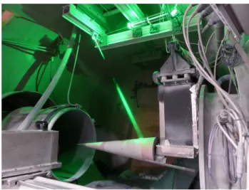
The model was fixated by a typical sting configuration and placed in a short distance downstream of the wind tunnel nozzle exit (see Fig. 1).
3.2 Pressure measurements 3.2.1 Surface pressure
The wind tunnel model was equipped with pressure holes with a diameter of 0.5 mm at nine different positions. Pres-sure tabs were located at three different axial sections along the model, at x=0.25, 0.495 and 0.651 m . In the first and
last section, four different tabs were positioned with an angu-lar distance of 45◦ . This setup enabled the analysis of model alignment and pressure gradients along the surface. The tabs were connected via steel and flexible tubing to a miniature electronic pressure scanner (ESP) outside the wind tunnel model with a measurement range of 34.5 kPa(5 psi). 3.2.2 Pitot pressure
The Pitot pressure was measured with a movable rake, con-sisting of five tubes, each with an inner and outer diameter of 0.2 and 0.4 mm , respectively. The distance between sub-sequent tubes was 1 mm . This multiple tube concept mini-mized the testing time for a highly resolved boundary layer profile. In wall-normal direction the rake was traversed with a linear actuator L4118L1804−T6X1 from Nanotec
Elector-nic GmbH & Co. KG, whereas the axial position was fixed during a test run. The motor was operated by a Nanotec
SMCI33-1 controller. The position of the probe was moni-tored with a Nanotec WEDL 5546 encoder. The actuator has a minimal step resolution of 5μm and a maximum speed of 20 mm/s . The rake movement during test time was stepwise
with corresponding settling times to ensure a sufficient fill-ing of the tube volumes. The Pitot tubes were connected via steel and flexible tubing to an ESP scanner with a meas-urement range of 103.4 kPa(15 psi) . The impact of potential interaction problems between the multiple tubes of the rake was tested with measurements via a single tube reference device. The differences fell within the corresponding uncer-tainties. To account for small run-to-run inflow differences, the pressure data of each run were first transformed to pres-sure coefficients via cp= (pPitot−p∞)∕q∞ . With the nominal
inflow values of static pressure p∞ and stagnation pressure q∞ according to Table 1, a corresponding Pitot pressure pPitot
was calculated and combined to a complete profile from sev-eral runs. The data from surface and Pitot pressure measure-ments were transformed to velocity profiles applying the
Rayleigh Pitot equation (see, e.g., Staff 1953) and assuming a Crocco–Busemann temperature distribution within the boundary layer (see, e.g., White 2006). The selection of the temperature distribution was based on a comparison between different approximations and numerical profiles for the cho-sen H2K flow conditions.
3.3 Particle image velocimetry 3.3.1 Setup
A particle image velocimetry setup was used to measure two-dimensional, two-component flow velocity fields. An ULTRA CFR Nd:YAG Laser System of the company Quantel was used as light source. It consisted of two pulse lasers which were superimposed and converted to a wave-length of ±532 nm . The frequency was set to 15 Hz for a
maximum energy of 191 mJ per pulse. The final laser sheet along the model surface had a nominal dimension of
60× (0.5−1.0)mm (streamwise length × thickness). The
setup inside the test section is visible in Fig. 1. To reduce wall reflections, the PEEK model wall was locally painted with red color in the vicinity of the laser sheet impact region. Additionally, the sheet was positioned so that most part of its extent was located on the camera-averted side of the model. For the acquisition of images, a PCO 1600 camera system was used, with a CCD chip of maximum resolution of 1600×1200 pix2 . The camera was positioned outside of
the test section, at a distance of approximately 2.1 m from
the model. A K2 DistaMax long distance microscope from the company Infinity Photo Optical was used. The chosen setup resulted in a magnification of M ≈0.99 . An optical
filter (wavelength 532±2 nm ) was mounted between the
objective and the CCD chip. With this setup a region of interest (ROI) of 9.0×12.0 mm2 (streamwise × wall-normal
distance) was obtained. The location of this ROI is described in Sect. 4. For seeding, a solid particle generator (SPG) was used, which was connected to the stilling chamber of the H2K wind tunnel. TiO2 particles of type 1002 from the
com-pany KRONOS INTERNATIONAL INC. were used. The manufacturer states a median diameter of dp≈0.2−0.3μm
and a density of 𝜌
p≈3800 kg/m3 . Before seeding, the
par-ticles were sieved and than dehydrated in an oven at 70◦C
for t>6 h to 12 h to prevent agglomeration (see, e.g., Ragni
et al. 2011). A dedicated sensitivity study of the particle
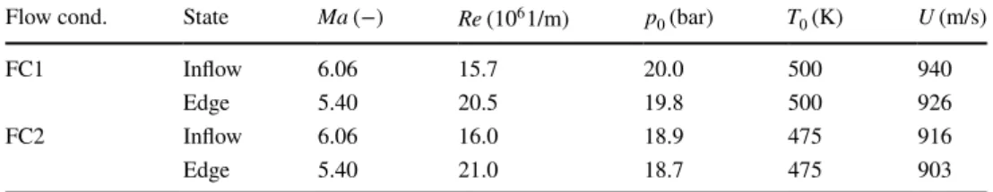
Table 1 Nominal flow
conditions FC1 and FC2 Flow cond. State Ma(−) Re(1061/m) p0(bar) T0(K) U(m/s)
FC1 Inflow 6.06 15.7 20.0 500 940
Edge 5.40 20.5 19.8 500 926
FC2 Inflow 6.06 16.0 18.9 475 916
property impact on the response behavior is given in Sect. 4. The timing of the PIV system was controlled via a Lab-Smith LC880 8-channel trigger box. The interframing time between two images was set to nominally tp=120 ns .
Dur-ing testDur-ing, a dependence of measured velocities on the laser power level was noticed. The time difference between two subsequent laser pulses was identified as the main contribu-tor to this deviation. A dedicated laser characterization with a photodiode setup was performed after the test campaign. This characterization resulted in corrected pulse distance values for all preset pulse distance and power level combi-nations used during the test campaign. The standard uncer-tainty of the extracted deviations was in the order of 1 ns or below and were included in the total PIV measurement uncertainty (see Sect. 4). A comparable influence was also reported in Williams (2014). The described setup typically resulted in a mean freestream displacement of Δx≈14.5 pix. 3.3.2 Analysis
All analyses were performed with the commercial PIV-view suite version 3.6.0. Approx. 200 valid PIV images were recorded per run. Several image pre-processing steps were conducted before analysis. Due to small model vibra-tions, a pattern matching algorithm was used to normalize all recorded images first. The wall was identified based on intensity images, averaged over all images per run. Profiles in the wall-normal direction, accumulated in streamwise direction, were used. A small rotation, typically below approximately 1◦ , was applied to align the surface with the
horizontal level. A background image subtraction was omit-ted since no significant improvement was noticeable.
For the processing of the images, several validation cri-teria were defined and correlated velocity vectors were not accepted if one of the following three criteria were not met. First, a normalized median filter with a threshold of 8 was applied on each vector along with its eight neighbors. Sec-ond, a dynamic mean test with a mean value of 2.0 and variance of 1.0 was applied. The third criterion was a mini-mum signal-to-noise ratio of each correlation peak of 5.0. An interrogation window size was accepted only if at each vector position at least 90% of the corresponding images met
the above criteria. The remaining single image non-accepted vectors were not included in further analysis (no interpola-tion was used). Based on these criteria, several single-grid and multigrid interrogation windows were chosen for further analyses (see Sect. 4). If not otherwise noted, an overlap of
50% was used. In all cases an algorithm was applied with
standard FFT correlation using Whittaker reconstruction sub-pixel peak fitting. Additionally, the algorithm used a multiple-pass interrogation method, which applied image deformation via cubic B-spline interpolation on all 3
selected steps, to compensate for high shear near the wall. Ensemble correlation analysis was applied to selected data.
3.4 Methods for skin friction approximation
For the analysis of the boundary layer velocity profiles, inner scaling is of interest (see Sect. 4). Since no direct meas-urements of the wall skin friction were performed, several different indirect approaches were compared. First, a fit-ting procedure, based on the law-of-the-wall, is presented. Additionally, the velocity gradient from the wall closest data points of the PIV measurements was exploited. Besides that, a modified integral method to approximate the compressible wall skin friction along the cone model was applied.
Fitting approach A procedure was applied to fit a meas-ured mean velocity profile onto the law-of-the-wall. In addi-tion to the logarithmic part, the wake part was also included using a Coles wake parameter formulation. The law-of-the-wall for a compressible turbulent boundary layer can be given according to White (2006):
Included are the effective velocity Ueff , derived from the
absolute, compressible velocity U by applying the trans-formation after Van Driest (see, e.g., Van Driest 1951,
1956; Berg 1977), the normalized wall normal distance
y+=√y
⋅U𝜏∕𝜈w , B as the law-of-the-wall constant chosen
with B=5.0 , 𝜅 as Karman constant chosen with 𝜅=0.4 , Π
as the wake strength parameter, usually depending on inflow and pressure gradient, and 𝛿 as the boundary layer thickness
(defined here by the wall distance where the velocity has reached 99% of the edge velocity). Including the wake for-mulation increased the amount of useful data points within the boundary layer, which in turn enhanced the quality of the fitting procedure. The applied method was originally introduced to study turbulent boundary layer profiles along smooth and rough walls by Berg (1977). The parameters necessary to fit are the skin friction velocity U𝜏 and the Coles
wake parameter Π . This method and its algorithm were
vali-dated against the data of Berg. Several consistency tests were performed by applying the fitting approach on PIV results derived with different interrogation windows (reported in Sect. 4.3) and on results from ensemble correlation. These tests resulted in a percentage change of the derived skin fric-tion velocities of ΔU𝜏 <1.3% , which showed only a small
sensitivity of the analysis to the investigated parameters. Additionally, it is a sign for the robustness of the fitting pro-cedure, since the results are only slightly affected by the amount of points within the profile, especially in the loga-rithmic region. The insensitivity of the fitting approach to the number of points is especially helpful for the analysis (1) U+ eff= Ueff U𝜏 = 1 𝜅ln(y + ) +B+Π 𝜅2 sin 2(𝜋 2 y 𝛿 ) .
of the Pitot data, which had a lower resolution than the PIV data.
Gradient approach If the velocity profile in the viscous sublayer close to the wall is available, the wall shear stress may be approximated by the velocity gradient at the wall. The high wall-normal resolution of the PIV interrogation windows 8×512 pix2 profiles (given as wall-normal ×
streamwise dimensions in pixel) enabled a distance from the wall for the first data point of iy(1) =4 pix which
corre-sponds to y(1) =0.03 mm , y∕𝛿(1) =0.0087 , y+(1) =1.79
which is located well within the viscous sublayer (see Fig. 5). Due to the derivation of the van Driest velocity transformation, its applicability is limited to the logarithmic layer (e.g., Fernholz and Finley (1980), Williams (2014)). For the viscous sublayer, an alternative velocity transforma-tion can be derived from the shear stress budget in the sub-layer with the assumption of negligible turbulent stress con-tribution, an exponential viscosity law with the exponent
𝜔=1 , the Crocco temperature distribution, 𝜕p∕𝜕x=0 and
constant wall temperature Tw according to Fernholz and
Fin-ley (1980). For the PIV data in this paper, both transforma-tions showed only minor differences in the sublayer, which fell below the corresponding uncertainties (see Sect. 4.3). Different developments to derive a scaling which is applica-ble to both, the viscous sublayer and log-layer, were dis-cussed, e.g., by Patel et al. (2016) and Trettel and Larsson (2016). Trettel and Larsson (2016) derived a scaling tested on supersonic channel and boundary layer cases with non-adiabatic wall conditions, including the effect of wall heat-ing. To categorize the impact of wall heating the authors derived a dimensionless parameter with Bq=qw∕(cpu𝜏Tw) ,
where qw represents the wall heat flux (negative, if wall is
heated) and cp the heat capacity at constant pressure. Low
absolute values of Bq represent near adiabatic conditions.
For boundary layer cases with || |Bq||
|<0.069, only small
dif-ferences between the introduced and the classical van Driest scaling were visible (see Trettel and Larsson 2016). For the boundary layer discussed in this paper, a value of |||Bq||
|≈0.02
can be approximated, based on infrared thermography data. This represents a case with only limited heating of the wall ( Tw∕Taw≈0.8 ) and therefore only limited differences to the
van Driest scaling are expected. Therefore, the van Driest scaled velocities were used in all following analyses. To esti-mate the shear stress, the wall closest velocity points were used to estimate the corresponding partial derivative by a difference quotient. The necessary wall viscosity 𝜇
w was
calculated via the Sutherland law based on the correspond-ing wall temperature from infrared thermography. The velocity difference was calculated for all points within y+<15 , assuming zero velocity at the wall.
Integral approach This method is based on an approach originally implemented to approximate the shear srtress
along a rough flat plate wall according to Latin (1998). For this approach, the momentum integral equation is solved in between two consecutive positions along the surface by implementing a functional dependence for the skin fric-tion coefficient of the kind cf,e=f(𝜃) (formulated with the boundary layer edge conditions). This function can be derived with the law of the wall solved at the boundary layer edge. In case of the rough version of the law of the wall along a flat plate, the resulting momentum integral can be solved analytically (Latin 1998). In case of a compressible smooth cone flow, an analytical solution is not possible any-more and need to be solved numerically. For the method, the validity of the law-of-the-wall needs to be assumed. Formu-lated at the boundary layer edge, Eq. 1 may be inserted into the compressible zero-pressure gradient momentum integral equation, which can be formulated along a cone with the assumption of constant edge conditions according to Fenter (1960). The resulting equation may be solved numerically with a Runge–Kutta solver with known initial values for boundary layer running length and momentum thickness. In this paper, the values were extracted from the first PIV (or Pitot) measurement section. The equations were iterated so that the resulting 𝜃2 matches the data at the second PIV
(or Pitot) measurement section at x2 . The influence of the
numerical step size Δx was tested and found to be
negli-gible for the conditions in this paper. The procedure was successfully cross-checked with the original implementation of Latin (1998) in a flat plate implementation. Additionally, the procedure was tested and validated with numerical data along a cone. The resulting percentage deviations of the skin friction coefficient was typically |Δcf,e|≤1.2%.
4 Results and discussion
Section 4.1 contains the nominal flow conditions of the conducted experimental test campaigns and the definition of measurement sections to extract boundary layer data. Then, numerical sensitivity studies are reported in Sect. 4.2. After the discussion of uncertainties and sensitivities, the experimental results of the mean velocities are compared to numerical and literature data in Sect. 4.3. Finally, the analy-sis of turbulence intensities from PIV measurements is dis-cussed based on numerical and literature data in Sect. 4.4.
4.1 Nominal flow conditions
Table 1 contains the nominal flow conditions of the wind tunnel campaigns. Two different flow conditions FC1 and FC2 were defined and details about the Mach number Ma, unit Reynolds number Re, reservoir pressure p0 , reservoir
temperature T0 and velocity U are given. The values are
In case of the inflow state ( ∞ ), U denotes the axial
veloc-ity, in contrast to the wall-parallel component in the rest of the paper. The inflow Mach number is derived from nozzle calibration, including viscous effects, depending on the Reynolds number. The reservoir conditions were directly measured, whereas the static conditions of the inflow were calculated via gas dynamic equations (e.g., Staff 1953). The uncertainties of the inflow parameters are based on calibrations of the corresponding instrumentation and can be given for the reservoir pressure with ±0.1% (full
scale of p0=70 bar ), reservoir temperature with ±1.1◦C
or ±0.4% (whichever is higher) and inflow Mach number
with ±0.04 . The nominal edge conditions were derived by
the Taylor–Maccoll equation (see, e.g., Anderson 1990), assuming negligible influence of a thin boundary layer. The two slightly different inflow conditions were designed to match the Mach and Reynolds number for different res-ervoir conditions. This was necessary due to infrastructure refurbishments of the H2K facility. The PIV measurement campaign was performed with FC1, and the Pitot cam-paign with FC2.
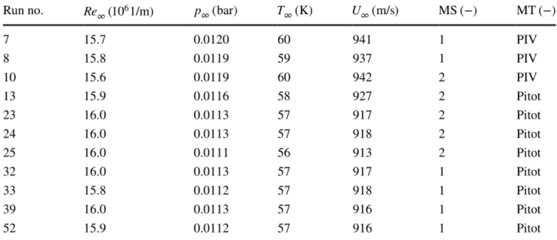
Table 2 contains detailed information for every reported run in this paper. The reservoir conditions of the con-ducted runs typically differ by less than approximately
1% from the nominal values. Run numbers from 7 to 10 correspond to the PIV campaign at FC1 and from 13 to 52 to the Pitot campaign at FC2. Only runs with suffi-cient quality with respect to inflow conditions and bound-ary layer measurements were chosen and included in this paper. The table contains the actual Reynolds number Re∞ ( Ma∞=6.06 for all runs), static pressure p∞ , temperature
T∞ and velocity U∞ . Additionally, the streamwise loca-tion for boundary layer profile measurements is given with measurement section MS1 or MS2 besides corresponding measurement techniques (MT). Locations for both meas-urement sections and measmeas-urement techniques are defined in Table 3 with the axial and the surface running length x
and s, respectively.
4.2 Numerical sensitivity studies
Dedicated sensitivity studies were performed on the hybrid axisymmetric mesh of the 7◦ cone model. The spatial
conver-gence was checked on three grid refinement levels via grid convergence index (GCI) according to Slater et al. (2000) and Roache (1994). The necessary parameters for a study with three grids ( i=1 : fine, i,j=2 : medium, i,j=3 : coarse)
were used according to Slater et al. (2000). All TAU code grid convergence computations were performed with the RSM model for fully turbulent flow and the nominal input parameters for FC1 and Tw=340 K (see Table 1). A nearly
constant refinement ratio of r≈1.5 was realized by globally
changing a pre-defined grid resolution in the complete field downstream the shock region. Additionally, the number of structured sub-grid layers along the wall was refined by an equal ratio (fine: 60 layers, medium: 40 layers, coarse: 27 layers). The corresponding order of convergence was calcu-lated to p=1.80 , which is close to the value p=1.75 ,
sug-gested by Rakowitz (2002) for TAU calculations with mixed first and second-order methods. The solution value to extract the GCI was the wall heat flux at MS1. The resulting conver-gence index between the finest and medium mesh resulted in GCI12=2.08% . The ratio GCI23∕(rpGCI12) =1.02 showed that the grid solutions were in the asymptotic range. Besides spatial convergence, the heat flux evaluation scheme, the height of first grid layer above the wall, reconstruction of gradients and turbulence model were considered. All influ-ences were finally added in quadrature and resulted in a total
Table 2 Test matrix Run no.
Re∞ ( 1061/m) p ∞ ( bar) T∞ ( K) U∞ ( m/s) MS (−) MT (−) 7 15.7 0.0120 60 941 1 PIV 8 15.8 0.0119 59 937 1 PIV 10 15.6 0.0119 60 942 2 PIV 13 15.9 0.0116 58 927 2 Pitot 23 16.0 0.0113 57 917 2 Pitot 24 16.0 0.0113 57 918 2 Pitot 25 16.0 0.0111 56 913 2 Pitot 32 16.0 0.0113 57 917 1 Pitot 33 15.8 0.0112 57 918 1 Pitot 39 16.0 0.0113 57 916 1 Pitot 52 15.9 0.0112 57 916 1 Pitot
Table 3 Streamwise locations of profile measurement sections for Pitot and PIV measurements
Name Pitot PIV
x ( mm) s ( mm) x ( mm) s ( mm)
MS1 492.3 496.0 490.3 − 499.3 493.9 − 503.0
variation of Δq̇ ≈13.2% , Δcf ≈9.2% ( ΔU𝜏≈4.6% ) and Δpw≈0.5% , which need to be accepted for TAU results on
the finest grid. The turbulence model variation had the big-gest impact with Δq̇ ≈10–13% . If not otherwise stated, all
results for comparison to experimental data were performed on the finest grid.
4.3 Mean flow velocity data
This chapter contains the results of the mean flow veloci-ties in the cone boundary layer extracted via Pitot pressure and PIV measurements. First, consistency, sensitivity and uncertainty checks of the PIV data are reported. Afterward, a synthesis for the profiles from both measurement techniques with numerical and literature data is given. Then, differ-ent approaches to extract the skin friction velocity from the Pitot and PIV data are presented and characterized, based on analytical and numerical data. Finally, the selected profiles are analyzed in inner and outer scaled form and discussed based on literature data.
4.3.1 Uncertainties and sensitivities
For the PIV data, general uncertainties from the setup, sensi-tivities to interrogation windows, wall temperature, particle slip and image number convergence were investigated. If not otherwise noted in this paper, combined uncertainties were derived by linear propagation of uncertainties. This uncer-tainty value represents a maximum level considering the most unfavorable and improbable case when all independ-ent influencing variables reach their minimum or maximum uncertainty value.
Setup The uncertainties for the flow velocities derived by PIV was estimated to ±2.5% based on the edge velocity.
The given final percentage difference is a propagated result of uncertainties for typical setup uncertainty, lens distortion, laser pulse timing and calibration reading error.
Interrogation window Sensitivity studies were performed with synthetic PIV images based on TAU RSM data of the cone flow to test the influence of the interrogation window (iw) size on the mean velocity profiles. Especially, the impact of stretched, high aspect ratio, interrogation win-dows was of interest. This type of window was selected to increase the wall-normal resolution, but at the same time ensure an acceptable amount of particles per interrogation window. This window shape is supported by the nature of the boundary layer with a much higher streamwise than wall-normal velocity magnitude. Interrogation window sizes were selected according to the analysis of the experi-mental data with 64×512 pix2 , 32×512 pix2 , 16×512 pix2
and 8×512 pix2 and multigrid analysis with 256×256 to 64×96 pix2 (published in Neeb et al. 2015) (given as wall-normal × streamwise dimensions in pixel). Valid results
could be extracted from the synthetic images for all tested interrogation windows. Only in the immediate vicinity of the wall ( y∕𝛿≈0.1 ), differences of pixel shift above Δdx=0.1 pix (corresponding to 0.7% of the edge
veloc-ity) were detected which were mainly caused by increased velocity gradients in this region. The drawback of using the aforementioned high aspect ratio interrogation windows is a limited resolution in the streamwise direction. Estimations based on TAU simulations resulted in an uncertainty below
ΔU∕Ue≈0.3%.
After utilizing synthetic images, the same interrogation windows were applied on the experimental data of run 7. Profiles in wall-normal direction were extracted at the mid-points in streamwise direction of the corresponding 2D vec-tor fields. All experimental profiles nearly collapsed, inde-pendent of interrogation window size, and the differences fell well below the corresponding uncertainties. Therefore, the interrogation window 8×512 pix2 was chosen to perform
all following mean velocity analyses due to its high resolu-tion in the wall-normal direcresolu-tion.
Wall temperature Due to the chosen wind tunnel model material PEEK, the wall temperature rose during a wind tunnel run by approximately 3–10% , corresponding to a
viscosity change of approximately 2–9% . This influence
was analyzed based on numerical calculations with chang-ing wall temperatures, accordchang-ing to the wind tunnel tests. An ensemble averaged velocity field from all temperature computations was compared to the velocity from a single calculation with a mean wall temperature. This resulted in an estimated maximal difference at MS1 of ΔU∕U≈0.5% ,
lim-ited to a region close to the wall for approximately y+<20 ( y∕𝛿 <0.1 ). This difference was included in the uncertainty
for the detailed analysis of viscous sublayer velocities (gra-dient approach for the friction velocity). For larger wall-normal distances, including the logarithmic layer (relevant, e.g, for the fitting for the friction velocity (see Sect. 4.3)), the difference dropped below ΔU∕U≈0.02% and was therefore
neglected.
Particle slip The finite particle response can have a major influence on velocities measured via PIV, especially in low density, hypersonic flows (Ragni et al. 2011; Wil-liams 2014). Simulations were performed with the particle module described in Sect. 2.2.1 to approximate the impact on the velocity profiles in the boundary layer under cur-rent experimental conditions. Since only manufacturer data for the used particles and no in situ measurements were available, sensitivity studies were performed to investigate the impact of these parameters on the particle response. On the one hand, the manufacturer values of the applied KRONOS 1002 particles for diameter and density were taken with dp1 =0.23μm and 𝜌p1=3800 kg/m3 , as
repre-sentative values for a state without any agglomeration. On the other hand, particle parameters with dp2 =2.0μm and
𝜌
p2=800 kg/m3 were used, according to Williams (2014),
approximating an agglomerated state. Williams derived these values experimentally for comparable TiO2 particles
at comparable particle Mach and Reynolds numbers. The particles were seeded into the TAU RSM flow solution at FC1 and Tw=360 K (see Sect. 4.2) and caught in a plane,
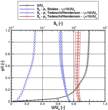
corresponding to MS1. Figure 2 contains the modulus of all relative particle velocity components ||𝐕
rel||= ( U2 rel+V 2 rel )0.5 (where, e.g., Urel=Up−U ), based on the streamwise edge
velocity component Ue to ||𝐕
rel||∕Ue for each caught particle p1 and p2 against the wall-normal distance, normalized by
the local boundary layer thickness 𝛿 . The collected particles
show negligible particle slip outside and near the boundary layer edge, whereas an increase toward the wall is visible. The maximum values are reached with |
|𝐕rel||∕Ue≈0.1% for
particle p1 and ||𝐕
rel||∕Ue≈2.1% for particle p2 . The
differ-ence in velocity is mainly driven by only weak successive deceleration of high-speed particles through the low-density boundary layer region. Although first decelerated by pass-ing the bow shock in front of the cone, high Knudsen num-bers and inertia effects lead to a persisting higher velocity than the surrounding fluid. This difference decreases with increasing running length, visible in Fig. 2 for the second measurement section MS2. Here the maximum relative velocity drops to ||𝐕
rel||∕Ue≈1.5% for particle p2.
Although on a noticeable level, the difference due to slip is not included in the general PIV uncertainty but kept in mind for later discussions. This decision was mainly based on the fact that only sensitivity values for the particle
parameters were available and so only a tendency could be estimated. Additionally, PIV measurements by Williams et al. (2015) and Williams et al. (2018), using comparable particles in a Ma≈7 boundary layer flow, show no sign of
slip influence on the mean velocity profiles, at least for a region including and above the logarithmic layer.
Image number convergence To check the convergence of the mean velocities, the cumulative mean of the streamwise velocity for different amounts of images N was analyzed at three positions outside the boundary layer. The extracted data between y∕𝛿=1.59−1.72 , including its uncertainties,
showed an agreement with the corresponding Taylor–Mac-coll edge velocity as reference for image numbers approxi-mately N>25 and nearly constant behavior above N≅150. 4.3.2 Comparison to literature data
Two Pitot probe profiles at measurement section MS1 and inflow condition FC2, processed to Mach numbers accord-ing to the procedure described in Sect. 3.2.2, are shown in Fig. 3. The Pitot measurements include a Mach number boundary layer region from approximately Ma=2 to an
edge value of approximately Ma=5.35 , which is in good
agreement with the nominal Taylor–Maccoll value for FC2, included as a black line (see also Table 1).
In Fig. 4, the velocities of the two PIV profiles at FC1 (run 7 and 8) are directly compared to the velocities derived from two Pitot pressure runs at FC2 (run 32&33 and 39&52 ), all extracted at the first measurement section MS1. Uncer-tainties are visualized by a gray area in case of the PIV and by error bars in case of the Pitot data (derived by propagation of uncertainties to ±1.7% of the edge velocity). Additionally,
|Vrel|/Ue [-] y/ δ [-] -0.1 -0.05 0 0.05 0.1 0 0.2 0.4 0.6 0.8 1 1.2 p1 (MS1) p1 (MS2) p2 (MS1) p2 (MS2) V
Fig. 2 Relative velocity difference of particles p
1 and p2 along the 7◦
cone at FC1 at measurement section MS1 and MS2 (shaded region corresponds to PIV setup velocity uncertainty)
Ma [-] y/ δ [-] 0 0.5 1 1.5 2 2.5 3 3.5 4 4.5 5 5.5 6 0 0.2 0.4 0.6 0.8 1 1.2 1.4 1.6 1.8 2
Run 32&33 (Pitot) Run 39&52 (Pitot) Mae,TM
different numerical data are included for comparison. TAU computations with different turbulence models (SAE, k-𝜔 and RSM) and three different inflow turbulent intensity lev-els are included at 0.1% (Tu nom., since it corresponds to the nominal value in TAU), 1% (Tu0.01) and 2% (Tu0.02). The latter two values represent a sensible range for the H2K facility, based on experiences in previous test campaigns and a turbulence characterization campaign with Laser 2 Focus (L2F). Additionally, DNS data of two turbulent boundary layer profiles along a flat plate at two different wall tem-peratures are included according to Duan et al. (2010). Both DNS profiles share the edge Mach number of Mae=4.97,
but the Reynolds numbers are Re𝜃=3819 ( Re𝛿2 =1526 )
and Re𝜃=4840 ( Re𝛿2=1537 ) for case M5T4 and M5T5,
respectively. The corresponding wall to adiabatic wall temperature ratios are Tw∕Taw≈0.7 and Tw∕Taw =1.0 . In
comparison, the Reynolds numbers extracted from the cur-rent experimental data are with Re𝛿2=635–1053 slightly
lower. The corresponding wall temperature condition is with Tw∕Taw≈0.8 enclosed by the M5T4 and M5T5 data
set. The skin friction coefficient of case M5T4 agrees with cf =1.5×10⁻³ close to the corresponding value of run 7 (see Table 4). All data are plotted in outer scaling.
The Pitot data as well as PIV data show excellent repeata-bility behavior within their corresponding uncertainty bands. In the upper parts of the boundary layer, above y∕𝛿 >0.3 , both measurement techniques show good agreement. For smaller wall distances, the Pitot data result in slightly higher values compared to the PIV data, although still covered by the corresponding uncertainties. A good agreement is visible for the upper part between experimental data and TAU com-putations, if the uncertainties are considered. Results with increased turbulence level of 1% (Tu0.01) and RSM turbu-lence model show best agreement, although deviations above the uncertainty band are visible below y∕𝛿≈0.1 . Sources
for this difference can be manifold. Possible contribution can arise from particle slip and increased shear close to the wall, previously identified as influencing factor for the PIV data. Despite the difference in Reynolds number, the DNS and experimental velocity profiles agree within the correspond-ing measurement uncertainties, except for a region between
0.05<y∕𝛿 <0.01 . This difference might be attributed to the difference in Reynolds number. The data of the second meas-urement section MS2 shows the same agreement between PIV and Pitot data (not shown here).
4.3.3 Friction velocity and inner scaling
To follow the suggested analyses given in the AGARD report 253 (Fernholz and Finley 1980), both Pitot pressure and PIV velocity profiles were transformed to inner and outer scaled form. Three approximations were applied and compared to extract the necessary skin friction velocity indirectly from the measured mean velocity profiles (see Sect. 3.4).
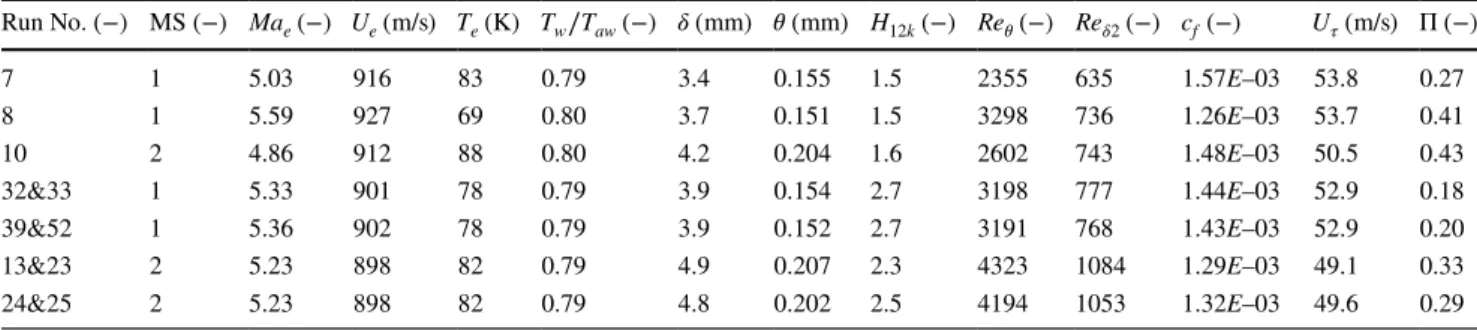
For this skin friction evaluation, different boundary layer edge and wall values were necessary for all approaches. These parameters were extracted from either the veloc-ity data or infrared data and are summarized separately in Table 4 for all investigated wind tunnel runs. The table
y/δ [-] U/ Ue [-] 10-3 10-2 10-1 100 101 0 0.2 0.4 0.6 0.8 1 1.2 TAU - RSM - Tu nom. TAU - RSM - Tu0.01 TAU - RSM - Tu0.02 TAU - k-ω - Tu0.02 TAU - SAE - Tu0.02 Duan2010 DNS M5T4 Duan2010 DNS M5T5 Run7 iw8x512 (PIV) Run8 iw8x512 (PIV) Run 32&33 (Pitot) Run 39&52 (Pitot)
Fig. 4 Streamwise mean velocity profiles from PIV (iw8×512 pix2 )
and from Pitot pressure at MS1 compared to numerical results (only every second experimental data point plotted for clarity, shaded region corresponds to PIV setup uncertainty, DNS data according to Duan et al. 2010)
Table 4 Edge and wall parameters of fitted Pitot and PIV ( 8×512 pix2 interrogation window) profiles at FC1 and FC2
Run No. (−) MS (−) Mae (−) Ue ( m/s) Te ( K) Tw∕Taw (−) 𝛿 ( mm) 𝜃 ( mm) H12k (−) Re𝜃 (−) Re𝛿2 (−) cf (−) U𝜏 ( m/s) Π (−) 7 1 5.03 916 83 0.79 3.4 0.155 1.5 2355 635 1.57E–03 53.8 0.27 8 1 5.59 927 69 0.80 3.7 0.151 1.5 3298 736 1.26E–03 53.7 0.41 10 2 4.86 912 88 0.80 4.2 0.204 1.6 2602 743 1.48E–03 50.5 0.43 32&33 1 5.33 901 78 0.79 3.9 0.154 2.7 3198 777 1.44E–03 52.9 0.18 39&52 1 5.36 902 78 0.79 3.9 0.152 2.7 3191 768 1.43E–03 52.9 0.20 13&23 2 5.23 898 82 0.79 4.9 0.207 2.3 4323 1084 1.29E–03 49.1 0.33 24&25 2 5.23 898 82 0.79 4.8 0.202 2.5 4194 1053 1.32E–03 49.6 0.29
includes the edge velocity Ue , the corresponding temperature Te from the Crocco-profile and additionally the
correspond-ing Reynolds numbers Re𝜃 and Re𝛿2 at the profile positions. The derived edge properties are consistent with each other within the corresponding uncertainties. The resulting Reyn-olds numbers are Re𝜃=2355–3298 and Re𝛿2=635–743 . According to the difference between the inflow condition FC1 and FC2, slightly different edge parameters were derived. This is in agreement with the expected values from Taylor–Maccoll for FC2 (see Table 1). The results of the three approaches to derive the skin friction velocity, the fit-ting, gradient and integral approach, are summarized and compared in Table 5. Where possible, the values include the corresponding uncertainties, stated in the following para-graphs. In case of the PIV data, only results from the inter-rogation window 8×512 pix2 are contained.
In general, very consistent skin friction velocities were extracted with an agreement between the different approaches and analytical and numerical data for each meas-urement section (MS) and flow condition (FC) if the corre-sponding uncertainties are accounted for (Table 5). The van Driest correlation was used for the analytical (see Sect. 2.1) and the TAU RSM results at 1% inflow turbulence intensity
(see Sect. 2.2) for the numerical comparison.
Fitting approach The skin friction velocities for run 7 and 8 show a good repeatability and the expected decrease for an increased running length for run 10 (Table 5). A slight difference in wall temperature between FC1 and FC2 is the reason for a slight difference in the derived skin friction velocities from Pitot data compared to the corresponding PIV results. This is in agreement with analytical or numeri-cal prediction. The uncertainties for the fitting and integral approach were determined by a Monte Carlo analysis due to the non-linearity of the methods. A sensitivity study showed
N=8000 samples to be sufficient for a converged result.
If not otherwise noted, uncertainties for input parameters were distributed uniformly which represents a conservative approach. The resulting uncertainties are given for a 95.4% confidence interval. An uncertainty of ±0.4 and ±3.4% of the
mean friction velocity was calculated for the Pitot and PIV data, respectively. The above stated values do include only procedural and no methodical uncertainties for the friction velocity. Methodical uncertainties can only be determined by comparing the results to a reference value of higher accuracy, either from experimental, numerical or analytical prediction. Most often, only cross-checks between different methods or comparison to analytical predictions are given in the literature. For the comparable Clauser chart method, which utilizes the velocity data and its slope only in the
Table 5 Summary of derived skin friction velocities at FC1 and FC2 and MS1 and MS2 [all values in ( m/s)]
MS FC Run no. Fitting approach Gradient approach Integral approach TAU van Driest
1 1 51.6 ± 2.9 52.7 7 53.8 ± 1.8 54.4 ± 4.9 8 53.7 ± 1.8 54.2 ± 4.9 7–10 50.7 ± 17.0 8–10 54.5 ± 18.3 1 2 50.1 ± 2.9 51.2 32&33 52.9 ± 0.2 39&52 52.9 ± 0.2 32&33–13&23 52.9 ± 3.0 32&33–24&25 51.0 ± 2.9 39&52–13&23 53.5 ± 3.1 39&52–24&25 51.6 ± 3.0 2 1 50.4 ± 2.9 51.4 10 50.5 ± 1.7 51.8 ± 4.7 7–10 49.2 ± 16.5 8–10 52.6 ± 17.7 2 2 49.0 ± 2.8 50.0 13&23 49.1 ± 0.2 24&25 49.6 ± 0.2 32&33–13&23 51.1 ± 2.9 32&33–24&25 49.5 ± 2.8 39&52–13&23 51.7 ± 3.0 39&52–24&25 50.0 ± 2.9
logarithmic layer, typical uncertainties of approximately 5%
are given in the literature for incompressible investigations (e.g. Purtell et al. 1981; So et al. 1994; Wei et al. 2005). For compressible investigations, the performance is typically stated within approximately 10% compared to analytical
predictions like van Driest (e.g., Berg 1977; So et al. 1994; Williams 2014; Peltier et al. 2016; Williams and Smits 2017; Williams et al. 2018). This is in agreement with observations in this paper (see Table 5).
Gradient approach The gradient approach was pos-sible to apply due to the wall-normal resolution of the
8×512 pix2 PIV profiles with the first point above the wall at y+(1) =1.79 which is located within the viscous sublayer
(see Fig. 5b). Typically, all skin friction velocity values derived by the gradient approach below y+=15 agreed
with the corresponding values from the fitting approach. This trend was detected for data from all interrogation win-dows reported above. Only the wall nearest point in case of the 8×512 pix2 profile was biased. Therefore, reported
skin friction values in Table 5 were derived by averaging all values within 8<y+<15 . The uncertainties for the
gradi-ent approach were evaluated based on linear propagation to
±9.1% based on a mean value.
Integral approach For the numerical integration of the von Karman equation, a step size of 0.1% of the difference
between 𝜃 at MS1 and MS2 was set by default. A systematic change of this step size showed a change of the resulting skin
friction coefficient of only Δcf,e<0.05% . In case of the PIV
data, two different combinations and in case of the Pitot data four different combinations were possible due to repeatabil-ity runs. The results, contained in the column named “inte-gral” in Table 5 show slight variations between the possible combinations at each flow condition. The corresponding values still agree with each other and values from the other approaches if the corresponding uncertainties are consid-ered. The combined uncertainties for the integral approach were evaluated to ±33.5 and ±5.7% for the PIV and Pitot
data, respectively. The higher uncertainty values in case of the integral approach from PIV data can be attributed to higher input uncertainties of edge Mach number, tempera-ture and momentum thickness.
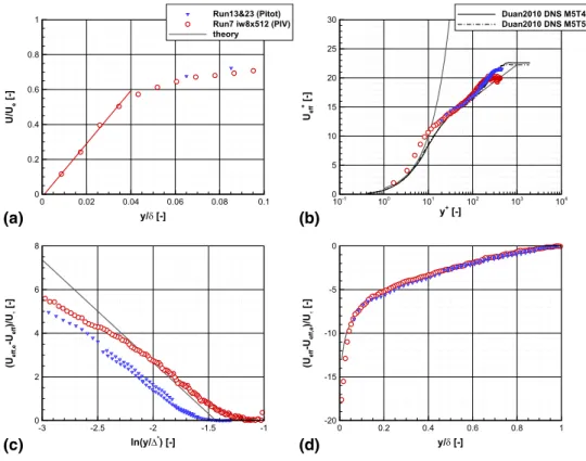
Due to the low uncertainty and consistent results, it was decided to use the skin friction and Coles wake parameter from the fitting approach to scale and analyze the PIV and Pitot profiles according to Fernholz and Finley (1980). The result for this scaling of the PIV data with 8×512 pix2 of
run 7 at MS1 is included in Fig. 5. The figure contains four different sub-plots a to d. In a, the profile is shown as nor-malized velocity U∕Ue against normalized wall-normal
dis-tance y∕𝛿 for a zoomed region close to the wall.
Addition-ally, a linear line is included which is fitted through data points y∕𝛿 <0.04 . In sub-plot b, the classical
law-of-the-wall with the van Driest transformed effective velocities U+
eff against y+ is included with one line for the viscous sub-layer Fig. 5 Streamwise mean
velocity data from PIV (iw8×512 pix2 ) and Pitot
pres-sure in inner and outer scaling according to Fernholz and Fin-ley (1980) (DNS data according to Duan et al. (2010)) y/δ [-] U/ Ue [-] 0 0.02 0.04 0.06 0.08 0.1 0 0.2 0.4 0.6 0.8
1 Run13&23 (Pitot)Run7 iw8x512 (PIV) theory (a) y+ [-] Ueff + [-] 10-1 100 101 102 103 104 0 5 10 15 20 25 30 Duan2010 DNS M5T4Duan2010 DNS M5T5 (b) ln(y/∆*) [-] (Ueff, e -Ueff )/U τ [-] -3 -2.5 -2 -1.5 -1 0 2 4 6 8 (c) y/δ [-] (Uef f -Ueff, e )/U τ [-] 0 0.2 0.4 0.6 0.8 1 -20 -15 -10 -5 0 (d)
( U+
eff=y+ ) and one line for the log-layer without wake (see
Eq. 1, neglecting the last term). Additionally, the two DNS profiles M5T4 and M5T5 according to Duan et al. (2010) are included in van Driest transformed inner-scaled form. In sub-plot c, an outer scaling is included with the dimen-sionless velocity defect as (Ueff,e−Ueff)∕U𝜏 against a
wall-normal distance y normalized by an integral length scale Δ∗ according to Fernholz and Finley (1980) and defined by
The theoretical curve in this sub-plot corresponds to the fol-lowing equation:
where M=4.7 and N=6.74 , which were derived based on
experimental data in zero-pressure gradient boundary layers, mainly along adiabatic walls (Fernholz and Finley 1980). The constants are strictly just valid for 1500<Re𝛿
2<40000 ,
but Fernholz and Finley (1980) showed also consistent analysis for data with Reynolds numbers below this range. In the fourth sub-plot, labeled d, a second outer scaling, represented by (Ueff−Ueff,e)∕U𝜏 against y∕𝛿 , is included. The theoretical curve is described, as given in Ekoto et al. (2008), by
The quality of the fitting procedure is directly visible by comparing the data points to the theoretical curves of the law-of-the-wall in Fig. 5b. All characteristic boundary layer parts are visible, like the S-shaped wake above y+
≈100 ,
the logarithmic layer for 100> ∼y
+>
∼10 and even the viscous
sublayer for data points with y+<10 . The first data point is
located well within the viscous sublayer. The linear charac-teristic of the sublayer is also visible in sub-plot a, compar-ing the line fit to the wall nearest data points. If compared to the DNS data in sub-plot b, a typical buffer layer is not visible for the current PIV data. One reason might be the particle slip, which was previously identified to be respon-sible for locally higher velocities in the near wall region (see paragraph particle slip in this section and Fig. 2). The wake portion of the run 7 profile was fitted best by a Coles wake parameter of Π =0.27 (see Table 4). Due to the low
Reyn-olds number, the wake parameter is lower than Π =0.55 ,
which is typically stated for an incompressible zero pres-sure gradient flow. This is well in line with data of other compressible flow investigations in a comparable Reynolds number regime (Fernholz and Finley 1980).
(2) Δ∗=𝛿 ∫ 1 0 ( (Ueff,e−Ueff) U𝜏 ) d(y 𝛿 ) . (3) (Ueff,e−Ueff) U𝜏 = −M⋅ln ( y Δ∗ ) −N, (4) (Ueff−Ueff,e) U𝜏 = 𝜅1⋅ln (y 𝛿 ) −2𝜅Π [ 1−sin2 (𝜋 2 y 𝛿 )] .
The outer scaling results of the run 7 data are con-tained in Fig. 5c, d. The theoretical curve in sub-plot d also depends on the wake parameter, so that an agreement with experimental data is a further consistency check. An excel-lent agreement between theory and data is visible down to wall-normal distances of y∕𝛿≈0.05 , corresponding to the
region of the viscous sublayer (see sub-figure a) for which the theory is not applicable any more. The outer scaling in sub-figure c shows good agreement between theory and data down to values of ln(y∕Δ∗) ≈ −2 . For lower wall distances,
the data points deviate from theory which was reported for low Reynolds number profiles at Re𝛿2 <2000 in Fernholz
and Finley (1980). This is consistent with the value range in this paper. To check if the flow is fully turbulent, despite low Reynolds numbers, the kinematic shape factor is a useful indicator, defined as the ratio of displacement and momentum loss thickness with the density set constant to H12k=𝛿∗k∕𝜃k . The PIV profile of run 7 with H12k≈1.5 (see
Table 4) lies in a value range characteristic for fully turbu-lent boundary layers at low to moderate Reynolds numbers (Fernholz and Finley 1980).
The same analysis was performed for velocity data derived from Pitot pressures of run 13&23 , also included
in Fig. 5. Although small, the dimension of the Pitot probe restricts the profile to a first wall-normal distance of
y(1) =0.32 mm , y∕𝛿(1) =0.082 , y+(1) =19.5 and therefore
almost one order of magnitude farther away from the wall, compared to PIV profiles. This is directly visible in sub-plot b, where the profile begins in the logarithmic part of the boundary layer. A small region of locally higher veloc-ity values compared to PIV and theory is visible. This was already visible in Fig. 4 and is most likely connected to near wall effects of the Pitot probe (Grosser (1996)), also visible in other investigations like Ekoto et al. (2007) or Sahoo et al. (2009). Besides this region, the profile shows acceptable agreement with the theory in the logarithmic layer. The outer scaled data in sub-plot d, which is driven by parameters like y∕𝛿 and Π , shows very good agreement with theory. Instead, the outer scaling in sub-plot c, driven by an integral length scale and therefore by near wall data, is parallel shifted from the theoretical line. This is mainly driven by the loss of near wall information due to the Pitot probe dimension. This is also noticeable with a shape factor of H12k=2.3 (see
Table 4), which is close to the value of a Blasius profile with H=2.59 and would erroneously indicate a laminar profile
(White 2006). To support this argument, a check was per-formed with an an artificial profile, derived by the law-of-the-wall, which was scaled to an edge velocity according to H2K conditions. Before using this artificial profile for the fitting analysis, the profile was intentionally cut below y∕𝛿=0.08 , comparable to the Pitot data. The corresponding
fitting results showed the same shift for the integral based profiles, as visible in Fig. 5c.
With the reported measurement techniques, a total num-ber of approximately 10 and 10–30 points in the logarith-mic layer are available for analysis from Pitot and PIV data, respectively. Additionally, the general agreement between the different skin friction velocity approaches and theory and numerics give confidence for a future analysis of rough wall data.
4.4 Turbulence data
Turbulence intensities were analyzed based on the PIV data. First, the impact of several influences and uncertainties is discussed. After that, data for the streamwise and wall-normal turbulence intensities are compared to literature and numerical data and the applicability of Morkovin’s hypoth-esis is tested.
4.4.1 Uncertainties and sensitivities
Several different influences can affect the extraction of tur-bulence intensities via PIV measurements (see, e.g., Adrian and Westerweel 2011). The influence of random errors, spatial resolution and particle lag filtering and convergence with image number has been analyzed and is discussed in the following.
Random error The impact of random errors was analyzed for selected interrogation windows. A strategy described in Williams (2014) and originally based on a work by Discetti et al. (2013) was followed, which utilizes two-point corre-lations in the streamwise direction derived from the instan-taneous velocity vectors of all recorded images. It is based on the assumption that random PIV measurement noise is statistically uncorrelated between non-overlapping interro-gation windows. Therefore, information from the correlation curve with a distance Δx greater than the overlap can be used
to extrapolate an unbiased value at zero distance. In this work, a linear fit was used, which tends to underestimate the error (Williams 2014), but an alternative parabolic fit was not feasible due to resolution.
Unfortunately, no random error could be extracted directly for the high aspect ratio interrogation windows with a streamwise extent of 512 pixel (as was used for the
pre-vious mean velocity discussion), since no non-overlapping points are available for the two-point correlation within the current ROI. Instead, a multigrid approach starting from 512×512 pix2 to a final size of iy×256 pix2 , with iy for
dif-ferent wall-normal dimensions, was used to approximate the error. Due to non-consistent two-point correlation curves, the results for windows with 8×256 pix2 and therefore also 8×512 pix2 were discarded for further analyses.
At the boundary layer edge, windows with 16×256 pix2 ,
32×256 pix2 and 64×256 pix2 result in random errors
of approximately 27 , 28 and 12% of the local turbulence
intensity, respectively. For the same interrogation windows, the analysis for points in the boundary layer resulted in ran-dom errors of approximately 27 , 19 , 13% at y∕𝛿≈0.8 and 65 ,
67 , 27% at y∕𝛿≈0.5 . For a reference value, a large
interro-gation window with a final size of 256×256 pix2 was used, restricted to the boundary layer edge due to its size. This window resulted in a random error of 5% . This decrease
of error with increasing window size could imply that the amount and distribution of particles in the flow is only suf-ficient for a moderate quality of turbulence data. Before a decision was made on the selection of window size, the sub-grid filtering was analyzed.
Sub-grid filtering The drawback of using larger inter-rogation windows to reduce random errors is an increased amount of sub-grid filtering. In this paper, this effect was estimated based on the work by Spencer and Hollis (2005), who performed analyses with synthetic and experimental data. Spencer and Hollis compared their results to theoretical curves by Host-Madsen and McCluskey (1994), who based their work on the assumption of homogeneous isotropic tur-bulence for particles within a single interrogation window. Both works investigated the impact of interrogation window size, but exclusively for an aspect ratio AR=1 . Since in this
paper windows with an aspect ratio AR≠1 were used, this
influence on the sub-grid filtering was analyzed separately, following the synthetic data approach by Spencer and Hol-lis (2005). Synthetic velocity fields with pre-defined mean velocities, Reynolds stresses and two-point correlations were created by applying digital filtering based on a technique introduced by Klein et al. (2003). The sub-grid filtering is approximated by spatial averaging the synthetic veloc-ity field, where the corresponding spatial box represents a simplified approximation of an interrogation window. This approach just simulates the filter characteristics without being influenced by typical additional factors of PIV analysis like, e.g., particle density or size distribution. See Spencer and Hollis (2005) and Klein et al. (2003) for further details of this approach. At this point, the symmetrical spatial box filter for averaging originally implemented by Spencer and Hollis (2005), was extended to an asymmetrical box, approx-imating interrogation windows with different aspect ratios. The approach was validated for windows with AR=1 with
the data of Spencer and Hollis (2005). Typically, inputs like mean velocities and Reynolds stresses were used as reported in Spencer and Hollis (2005). Additionally, values for mean velocities, Reynolds stresses, field size and number of fields were varied and the influence on the results was found to be negligible.
The synthetic two-point correlation was prescribed by an exponential distribution, defined by a prescribed integral length scale Lu′u′ (see Spencer and Hollis (2005)). A value
for this length was based on literature data, since the limited PIV ROI and resolution of the data in this paper prohibited

![Table 5 Summary of derived skin friction velocities at FC1 and FC2 and MS1 and MS2 [all values in ( m/s)]](https://thumb-us.123doks.com/thumbv2/123dok_us/1878977.2774269/11.892.78.811.607.1072/table-summary-derived-skin-friction-velocities-fc-values.webp)