Component-Based Aerodynamic Shape Optimization using Overset Meshes

(1)

Component-Based Aerodynamic Shape Optimization

using Overset Meshes

by Ney R. Secco

A dissertation submitted in partial fulfillment of the requirements for the degree of

Doctor of Philosophy (Aerospace Engineering) in the University of Michigan

2018

Doctoral Committee:

Professor Joaquim R. R. A. Martins, Chair Assistant Professor Jesse S. Capecelatro Professor Carlos E. S. Cesnik

(2)

(3)

Ney R. Secco [email protected] ORCID iD: 0000-0001-6799-2452

(4)

(5)

ACKNOWLEDGEMENTS

This work would not be possible without the help of many people that assisted and inspired me along the way.

First I thank my advisor, Prof. Martins, for giving me opportunity to join the MDO Lab. His mentorship made me a better researcher and a better person. I learned valuable lessons that I will take for my entire life.

I also acknowledge Prof. Jesse Capecelatro, Prof. Carlos Cesnik, and Prof. Karthik Duraisamy for serving as committee members. I appreciate your time considering this work and providing helpful suggestions.

MDO Lab members were also essential for the accomplishment of this work. Dr. Gae-tan Kenway’s work was the foundation for what I developed in this thesis. Dr. John Hwang showed me the first steps on using the MDO Lab codes and also provided helpful discus-sions. John Jasa helped with the implementation of the pySurf module. I am also grateful for meeting great friends in the MDO Lab: Anil Yildirim, Charles Mader, David Bur-dette, Eirikur Johnson, Josh Anibal, Justin Gray, Nicholas Bons, Song Chen, Shamsheer Chauhan, Sicheng He, and Timothy Brooks.

My wife, Claudia, encouraged me to face the challenge of studying abroad. She also kept me focused during moments of pressure. I am forever thankful for your patience and for being always there whenever I needed someone to count on. I thank my family for being always supportive in every step of my life and for giving me confidence and strength to overcome difficulties.

(6)

I express my gratitude towards Prof. Bento Mattos, my advisor during the undergrad-uate and Masters course at the Instituto Tecnolgico de Aeronutica (ITA), since he played a vital role in introducing me to Aircraft Design and MDO. I also thank the Brazilian Air Force for providing the necessary funding for this work.

(7)

LIST OF FIGURES

1.1 Comparison of shock waves (top) and trailing edge separation (bottom) be-tween the baseline and optimized configurations of the TBW optimization us-ing multiblock structured meshes. The previous optimization could not com-pletely remove shocks and separation near junctions. . . 2

1.2 Skewed cells on the surface mesh (black) and volume mesh (red) of a truss-braced wing configuration using a patched multiblock mesh. . . 6

1.3 Hole cutting of a cylinder mesh overlapping a Cartesian background mesh. . . 7

1.4 Collar meshes are necessary to ensure valid cells along intersections. . . 8

2.1 Steps for generating collar mesh for a wing-fuselage junction. pySurf is re-sponsible for steps a–c. The mesh extrusion module used in step d (pyHyp) is covered in Sec. 3.3. . . 17

2.2 Additional features implemented in the collar marching scheme to improve mesh quality for CFD analyses. . . 20

2.3 Representation of a generic subroutine and its corresponding AD versions. . . 20

2.4 Intersection between triangles of two components. . . 24

2.5 Low-wing configuration shifted to high-wing configuration with automatically generated collar meshes for the CRM geometry. . . 27

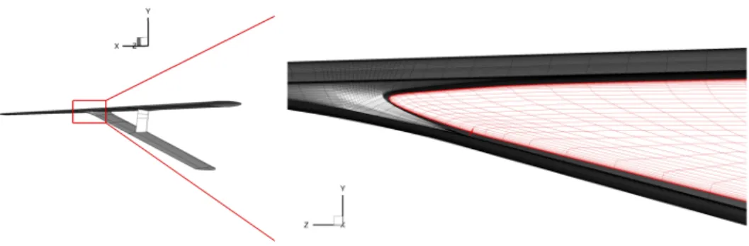
2.6 Aft view of the CRM wing-body junction. The left figure shows the design variable definition and the tracking of the trailing edge intersection point. The figure on the right shows how surface mesh points move as the wing is trans-lated. The red arrows indicate the AD-computed derivatives for the trailing edge intersection position (left) and surface mesh points (right) as we ver-tically translate the wing. The computed gradients for triangulated surface intersections are smooth and accurate enough for gradient-based optimization. 27

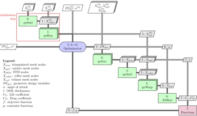
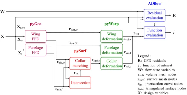
3.1 XDSM of the overall optimization framework. The initialization step gener-ates the reference volume nodes for the mesh deformation. . . 30

3.2 Hyperbolic extrusion of the surface meshes into volume meshes for a wing-body configuration. . . 32

3.3 Symmetry plane showing the fuselage near field mesh (red) the wing near field mesh (blue) and the background mesh (black) made by a Cartesian block and an O-mesh. . . 33

(10)

3.5 Zipper meshes are used to fill the gaps among overlapped meshes for force integration. They are not employed during the flow solution. . . 35

3.6 Subset of the framework subroutines required for the computation of CFD residuals (R) and functions of interest (f). . . 39

3.7 Derivative backpropagation chain. The modules represented here are the re-verse counterparts of the modules shown in Fig. 3.6. The plus signs indicate that the derivative seed should be accumulated from multiple sources. Sub-scripts ‘w’, ‘f’, ‘c’, and ‘aero’ indicate that quantities refer to wing, fuselage, collar, and flow conditions, respectively. . . 39

3.8 Transonic configuration used for wing translation study. Theywingdesign

vari-able controls the vertical displacement of the wing. . . 40

3.9 Drag variations due to the vertical translation of the wing of the transonic airplane configuration of Fig. 3.12. The red arrows represent gradients. We observe noise at small steps (on the right), but the gradients are still consistent with the overall trend. . . 41

3.10 Effects of the CFD mesh refinement on the noise levels for the same wing translation problem shown in Fig. 3.12. The noise levels are smaller when we use finer versions of the CFD structured meshes. . . 41

3.11 Optimization path for the wing translation problem. The plot on the right is a zoomed-in view showing the last iterations of the optimizer. The optimizer is trapped in a valley caused by the noise, but it manages to improve the baseline design. . . 42

3.12 Transonic configuration used to study wing translation. The design variable

∆xwing controls the horizontal displacement of the wing. . . 44

3.13 Variations in drag for different horizontal wing positions normalized by the fuselage diameter (Dfuse). The right plot shows drag variations for small dis-placements. The noise caused by changes in overset connectivity decreases as the mesh is refined. . . 44

4.1 Wing FFD showing the control points (red dots), which are manipulated by the twist and vertical displacement variables. . . 46

4.2 Pairs of points used to define thickness constraints. The distance between the pair of points cannot decrease during the optimization. . . 47

4.3 Fuselage FFD showing the free control points as blue dots. The other control points remain fixed to guaranteeC1continuity within the undeformed region. . 47

4.4 Structured surface meshes used for the volume mesh extrusion. The primary component meshes (wing and fuselage) are shown in black, and the automati-cally generated collar mesh is shown in red. . . 50

4.5 Wing-body junction flow patterns predicted by ADflow for the DLR-F6 con-figuration. The baseline geometry shows separation on the junction trailing edge (left), while the addition of the FX2B fairing removes it (right). This is the same trend observed in DPW3.. . . 50

4.6 Effect of grid refinement and turbulence model variant in the recirculation bubble size. . . 52

(11)

4.7 Drag convergence study for the DLR-F6 configurations. N represents the number of cell in the CFD mesh. Blue colors refer to the baseline DLR-F6 configurations and red colors refer to the DLR-F6-FX2B configuration. . . 52

4.8 Effect of refinement of triangulated surface over CFD results. The coarse tri-angularization is used for optimization. . . 53

4.9 Fairing-only optimization history. Some normal displacement design variables went to the lower boundary of0.04m. . . 54

4.10 Optimized fairing for the fairing-only optimization (Problem F). . . 55

4.11 Wing-body junction flow before and after the fairing optimization (Problem F). Red regions indicate reversed flow. The redesigned fairing reduces the recir-culation bubble. . . 55

4.12 Comparison of lift and drag distributions between the baseline (B) and the fairing-optimized configuration (F). . . 56

4.13 Relative computational time of the tasks performed during and optimization iteration involving an adjoint solution. The average time of the iteration is of 85 seconds. . . 57

4.14 Progression of the optimized drag value due to the additional active design variables. Drag decreases as we add more degrees of freedom to the optimization. 57

4.15 Rear views comparing the fairing sizes obtained for different optimizations. The fairing gets smaller as the optimizer gets more control over the wing prop-erties. . . 58

4.16 Contour plot showing the distance that the fuselage surface moved during op-timization. The fuselage surface moves a relatively large amount when the optimizer can only control the fairing. . . 58

4.17 Optimization histories for the F+T and F+T+S problems. The fairing design variables do not reach the upper bound in either problem. . . 59

4.18 Comparison between lift and drag distributions for all fairing optimizations. The inclusion of twist variables (T) allows the optimizer to achieve more effi-cient lift distributions, which are closer to an elliptical one. . . 60

4.19 Pressure coefficient slices of all optimized configurations. The optimizer de-signs wings with smoother pressure distributions as we activate wing shape variables (S). The shock on the upper wing surface is also removed by the shape variables. Even though Problems T+S and F+T+S have different de-sign spaces, they show similar airfoils and pressure distributions since they converged to practically the same wing design. . . 61

4.20 Wing-body junction trailing edge after every optimization problem. Red re-gions indicate reversed flow. The redesigned fairings eliminate the recircu-lation bubble in all problems. The wing shape variables achieve smoother chordwise pressure distributions. . . 62

4.21 Comparison between the optimized configuration with and without fairing de-sign variables. Optimization without the fairing dede-sign variables still shows trailing edge separation region (red). . . 62

(12)

4.22 Comparison between lift and drag distributions of the twist and shape opti-mized configurations with (F+T+S) and without (T+S) fairing variables. The resulting twist and airfoil distributions get progressively more similar as we move towards the tip. The F+T+S configuration has a smaller drag in this region as well, which leads to the improvement seen in Fig. 4.14. . . 63

4.23 Mesh refinement study for baseline (B) and optimized configurations (F and F+T+S). Dashed lines represent continuum estimates. The optimized design improvements are still present at finer mesh levels. . . 63

5.1 Baseline SBW configuration of the PADRI 2017 workshop. Views are not in the same scale. . . 67

5.2 Structured surfaces meshes of the primary components of the aircraft. The O-grids near intersections increase the cell density to facilitate the overset hole cutting process. . . 69

5.3 Triangulated surfaces used for intersection detection and collar mesh generation. 69

5.4 FFD boxes of the primary components whose shape will be optimized. The dots represent the FFD box control points. . . 70

5.5 Points of the wing (blue) and strut (red) where thickness constraints are en-forced. The distances between the pair of points cannot go below their initial value. . . 71

5.6 Optimization history of the SBW optimization. The drag decreases by 33 counts for the same lift coefficient.. . . 72

5.7 Comparison of shock and pressure distributions between the baseline (left) and optimized (right) designs. The strut is shown at a different scale. . . 73

5.8 Separation on the trailing edge of the wing-strut junction before (top) and after (bottom) the optimization. . . 73

5.9 Spanwise distribution of lift, drag and twist for the baseline (dashed lines) and optimized configuration (solid lines). The strut generates downward lift, and the inboard region of the wing increases its lift distribution to compensate for that, yielding an overall elliptical lift distribution. . . 74

5.10 Component-wise lift distribution. The lift is normalized by theCLconstraint. . 74

5.11 Cross-sectional slices of the wing and strut and corresponding pressure distri-butions for the baseline (dashed lines) and optimized (solid lines) configurations. 75

5.12 Cross-sectional slices of the vertical segment of the strut for the baseline (dashed lines) and optimized (solid lines) configurations. . . 76

5.13 Optimization history of the SBW optimization for the PADRI 2017 guidelines. The drag decreases by 14 counts while maintaining the same lift coefficient of the baseline configuration (red line). . . 77

5.14 Discrepancies between the CFD surface nodes of the baseline (black) and op-timized (red) configurations only occur on the lower surface of the wing and on the strut surface within the specified spanwise range. . . 78

5.15 Comparison of shock waves between the baseline (left) and optimized (right) designs for the PADRI optimization case. Shocks still remain outside of the optimized region. . . 78

(13)

5.16 Rear view of the wing-strut intersection showing separation regions (blue). The optimizer manages to remove the trailing edge separation only within the spanwise range where the design variables are active. . . 78

5.17 Comparison among the cross-sectional slices of the wing and strut and cor-responding pressure distributions for the baseline configuration (red dashed lines), the fully optimized configuration (red solid lines), and the optimized configuration for the PADRI guidelines (black). The optimized shape for the PADRI 2017 case has more twist to compensate the fixed twist angles of the wing and the remainder of the strut. . . 79

6.1 Execution order of the MACH framework modules during each optimization iteration (black lines) and summary of the modifications done to these modules as part of this thesis (in red). The dashed lines indicate processes that are only executed in the initialization step of the optimization. . . 84

6.2 Possible applications for the component-based parametrization technique de-veloped in this thesis. . . 86

A.1 Meshes marched with different splay factors. The red line is the baseline curve for the marching process. . . 96

A.2 The use of blending factor (ν = 0.5) avoids highly skewed cells where guide curves are oblique to the intersection line. . . 98

(14)

LIST OF TABLES

4.1 DLR-F6 aerodynamic shape optimization problem. . . 46

4.2 Identification tags for each optimization problem. . . 48

4.3 Inputs required by pySurf; these are generated by ICEM CFD using the origi-nal IGES representation of the DLR-F6 model. . . 48

4.4 Mesh levels used for drag convergence study. The maximum y+ _{values are}

computed based on the converged CFD results. . . 51

4.5 Aerodynamic coefficients obtained for each optimization. . . 57

5.1 Geometric characteristics and flight conditions used for the baseline SBW con-figuration analysis. . . 68

5.2 SBW aerodynamic shape optimization problem.. . . 70

(15)

LIST OF ABBREVIATIONS

AD algorithmic differentiation

ADT alternating digital tree

API application programming interface

ASO aerodynamic shape optimization

BLI boundary layer ingestion

CAD computer aided design

CDGT conceptual design geometry tools

CFD computational fluid dynamics

CRM common research model

DPW3 Third Drag Prediction Workshop

DPW6 Sixth Drag Prediction Workshop

FFD free form deformation

IDW inverse distance weighting

IHC implicit hole cutting

LAPACK linear algebra package

MACH multidisciplinary design optimization of aircraft configurations with high fidelity

NURBS non uniform rational basis splines

OML outer mold line

PADRI Platform for Aircraft Drag Reduction Innovation

PDE partial differential equations

(16)

RANS Reynolds-averaged Navier–Stokes

SA Spalart–Allmaras

SNOPT Sparse Nonlinear Optimizer

SBW strut-braced wing

SUGAR Subsonic Ultra-Green Aircraft Research

TBW truss-braced wing

VLM vortex-lattice method

(17)

ABSTRACT

Advances in computational power allow the increase in the fidelity level of analysis tools used in conceptual aircraft design and optimization. These tools not only give more accurate assessments of aircraft efficiency, but also provide insights to improve the perfor-mance of next-generation aircraft. Aerodynamic shape optimization involves the inclusion of aerodynamic analysis tools in optimization frameworks to maximize the aerodynamic efficiency of an aircraft configuration via modifications of its outer mold line.

When using CFD-based aerodynamic shape optimization, generating high-quality struc-tured meshes for complex aircraft configurations becomes challenging, especially near junctions. Furthermore, mesh deformation procedures frequently generate negative volume cells when applied to these structured meshes during optimization. Complex geometries can be accurately modeled using overset meshes, whereby multiple high-quality structured meshes corresponding to different aircraft components overlap to model the complete air-craft configuration. However, from the standpoint of geometry manipulation, most methods operate on the entire geometry rather than on separate components, which diminishes the advantages of overset meshes.

Tracking intersections among multiple components is a key challenge in the implemen-tation of component-based geometry manipulation methods. The mesh nodes should also be updated in accordance to the intersection curves.

This thesis addresses this issue by introducing of a geometry module that operates on individual components and uses triangulated surfaces to automatically compute intersec-tions during optimization. A modified hyperbolic mesh marching algorithm is used to

(18)

regenerate the overset meshes near intersections. The reverse-mode automatic differen-tiation is used to compute partial derivatives across this geometry module, so that it fits into an optimization framework that uses a hybrid adjoint method (ADjoint) to efficiently compute gradients for a large number of design variables. Particularities of the automatic differentiation of the geometry module are detailed in this thesis.

By using these automatically updated meshes and the corresponding derivatives, the aerodynamic shape of the DLR-F6 geometry is optimized while allowing changes in the wing-fuselage intersection. Sixteen design variables control the fuselage shape and 128 design variables determine the wing surface. Under transonic flight conditions, the opti-mization reduces drag by 16 counts (5%) compared with the baseline design.

This approach is also used to minimize drag of the PADRI 2017 strut-braced wing benchmark for a fixed lift constraint at transonic flight conditions. The drag of the opti-mized configuration is 15% lower than the baseline due to reduction of shocks and sep-aration in the wing-strut junction region. This result is an example where high-fidelity modeling is required to quantify the benefits of a new aircraft configuration and address potential issues during the conceptual design.

The methodologies developed in this work give additional flexibility for geometry and mesh manipulation tools used in aerodynamic shape optimization frameworks. This ex-tends the applicability of design optimization tools to provide insights to more complex cases involving multiple components, including unconventional aircraft configurations.

(19)

CHAPTER 1

Introduction

Fuel-burn reduction is one of the main drivers in aircraft design due to environmental and economical reasons. Improvements in computational power allow designers to increase the fidelity level of aerodynamic and structural analysis used during aircraft conceptual design. These tools can be assembled in optimization frameworks to reduce fuel burn and to increase the profitability of future aircraft designs.

The use of high-fidelity analysis tools is also paramount for the design of uncon-ventional aircraft configurations. An important feature of these tools is that they simu-late additional phenomena compared to low-fidelity tools. For instance, the vortex-lattice method (VLM) cannot capture shock waves nor flow separation [1], while these features can be quantified in Reynolds-averaged Navier–Stokes (RANS) simulations. The results of the former can be corrected via regressions based on experiments and historical data for conceptual design applications. However, the lack of information for unconventional air-craft prevents the use of this approach for this type of airair-craft. In this situation, the use of high-fidelity analysis poses as a cost-effective solution to gather data with enough accuracy for conceptual design purposes.

High-fidelity analysis also considers the entire outer-mold line of the airplane instead of the simplified representations used in low-fidelity tools. For instance, wings are condensed to a single surface following its mean camber line for the VLM, while the actual wing shape (upper surface, lower surface, and trailing edge) can be modeled inRANSanalysis. As shapes become more detailed, we need more sophisticated methods to parametrize and manipulate these shapes.

Multiple examples of Euler- and RANS-based design optimizations are reported in the literature. These techniques are usually used to optimize relatively simple geometries, such as airfoils [2–4] or isolated wings [5–8].

For complex configurations, the design variables usually operate on a limited portion of the geometry [8–10]. For example, Merle et al. [10] optimized a conventional aircraft

(20)

configuration subject to trim constraints. Even though they simulated the aerodynamics of the entire aircraft configuration (wing, fuselage, tail, nacelle, and pylon), the shape design variables only modified the wing. In addition, they had to damp wing shape deformations near the wing-fuselage intersection to avoid discontinuities in the surface mesh. These simplifying assumptions limited the space of possible geometries and design variables, such as the wing mounting angle [9].

Ivaldi et al. [11] optimized a truss-braced wing (TBW) configuration with RANS anal-ysis. This is a relatively complex configuration due to the presence of interconnected com-ponents. The limitations of the geometry manipulation tool used in this work prevented the definition of design variables near junctions. Therefore, the optimized configuration still showed shock waves and flow separation in these regions (Fig.1.1).

Figure 1.1: Comparison of shock waves (top) and trailing edge separation (bottom) be-tween the baseline and optimized configurations of the TBW optimization using multi-block structured meshes. The previous optimization could not completely remove shocks and separation near junctions.

The challenges that hindered the optimizations discussed above are twofold: first, the geometry manipulation tools operated on the entire configuration at once instead of us-ing component subdivision information to simplify the definition of the design variables. Second, the optimization frameworks could not track changes in the intersections among components to appropriately update the meshes used for aerodynamic analysis. Therefore, the potential of optimization methodologies to gain design insights was not fully explored, especially regarding junction design and simultaneous optimization of multiple compo-nents.

This impacts the design optimization of unconventional aircraft designs that rely on ef-ficient interactions among multiple components. For instance, the aerodynamic efficiency of the high-aspect ratio wing of a TBW configuration may be hampered by the interfer-ence drag caused by the additional components. The tail-cone thruster configuration also

(21)

requires synergy among its components [12–14], since the position of the vertical tail and the rear fuselage shape interfere on the inlet properties of the rear fan.

This thesis focuses on expanding current geometry and mesh manipulation tools to fa-cilitate the use of aerodynamic shape optimization (ASO) methodologies for complex con-figurations. This includes tracking intersections among components within the optimiza-tion process and updating the meshes for the new shape. This thesis also demonstrates that these methods can be differentiated and integrated in gradient-based optimization frame-works.

1.1 High-fidelity aircraft design optimization

Aircraft design is a multidisciplinary problem with a large number of degrees of freedom. Covering this design space solely based on experimental and flight data would be extremely expensive. Therefore, aircraft designers resort to computational tools to prospect most of the design space and narrow down a handful of configurations for posterior design phases, while experiments are used to complement and verify results from the computational frame-work [15]. Once the execution of these computational tools are streamlined for automatic evaluation of multiple aircraft designs, optimization becomes possible.

Optimization algorithms can be classified in two groups: free and gradient-based algorithms. Zingg et al. [16] and Yu et al. [17] compare these two approaches for aerodynamic shape optimization applications. Gradient-free optimization algorithms need access only to the inputs and outputs of the design functions (objectives and constraints), so the analysis framework can be used as is, without any additional implementation. Examples of gradient-free algorithms are genetic algorithms [18], particle swarm optimization [19], and the Nelder-Mead simplex [20]. However, the number of function evaluations necessary to converge an optimization problem to a given tolerance dramatically increases with the number of design variables [21], making this approach unfeasible for cases with expensive function evaluations and more than few dozen design variables.

Gradient-based optimization algorithms use gradients of the functions of interest to di-rect the search for the optimum design point [22]. The convergence rate of these algorithms has a weaker dependence on the number of design variables, making them suitable for op-timization problems with hundreds of design variables, which is usually the case forASO

problems. On the other hand, the efficient computation of gradients is not a straightfor-ward task, and it usually requires additional implementation efforts. Peter and Dwight [23] provide a detailed review of gradient computation methods applied toASO.

(22)

modification to the analysis code used to compute the functions of interest. However, the step size for best accuracy is problem-dependent and also bounded by truncation and sub-tractive cancellation errors [24]. The complex-step method [25] overcomes the subtractive cancellation issues, thus giving machine-precision-accurate derivatives, but it suffers from the fact that the number of function evaluations required to compute gradients scales lin-early with the number of design variables, just like finite difference.

Algorithmic differentiation (AD) is an alternative method to compute gradients in which the chain rule of derivatives is applied line by line of the analysis code [24], either via oper-ator overloading or source code transformation. The analysis code can be differentiated in two modes: the forward AD mode, in which the chain rule products are performed from in-puts to outin-puts, and the reverse AD mode, in which the chain rule products are constructed from outputs to inputs.

Both methods allow the computation of the Jacobian matrix that correlates inputs (de-sign variables) and outputs (functions of interest) of the analysis code. However, each call to the forward AD code provides a column of the Jacobian matrix, while a call to the re-verse AD code provides a row of the Jacobian matrix. Thus, the number of total calls of the forward AD code to assemble the full Jacobian matrix is equal to the number of design variables (similarly to finite difference and complex-step), while the total number of calls for the reverse AD code is equal to the number of functions of interest [26]. Since the num-ber of design variables inASOproblems is higher than the number of functions of interest, the reverse AD mode is suitable for efficient gradient computation [23].

The reverse mode AD requires the storage of intermediate values of variables used throughout the code. For instance, in the case of iterative solvers used in computational fluid dynamics (CFD), this amounts to storing the flow state variables of every iteration, leading to prohibitive memory requirements. The discrete adjoint method circumvents this issue since it allows derivative computations across the CFDmodule based solely on the converged flow state variables.

The discrete adjoint equation is a linear system whose elements are partial derivatives of theCFDresiduals and function of interest with respect to the flow state variables. These partial derivatives can be computed using reverse AD, and only the residual evaluation function of the CFD solver needs to be differentiated, leaving the iterative methods outside of the reverse AD chain. This combination of reverse AD and the discrete adjoint method is called the hybrid adjoint method (or ADjoint) [27]. The implementation of the hybrid adjoint method will be further discussed in Chapter3.

Multiple applications of the hybrid adjoint method are present in the literature for dif-ferent fidelity levels of aerodynamic and structural analysis. Elham and van Tooren [28]

(23)

use the hybrid adjoint method for a VLMcode. Mader et al. [27] describe the hybrid ad-joint method applied to the Euler equations. Brezillon and Dwight [29] use the adjoint formulation for a RANS solver, but turbulence model variables were assumed as constants in the differentiation process since some partial derivatives were computed by hand or with finite-differences. Lyu et al. [30] include the turbulence model in the AD process to use the hybrid adjoint method with RANS equations while including turbulence model sensitivity. Dumont and M´eheut [8] show another example of discrete adjoint application to RANS equations in which they use a time marching scheme to converge the adjoint system.

Burdette [31] demonstrated that an aircraft optimized based on Euler equations and semi-empirical regressions for viscous drag estimation performs poorly when analyzed with RANS equations, justifying the efforts in increasing the fidelity level of the analy-sis code used in aircraft design optimization. This is specially important to obtain more accurate performance estimates of unconventional aircraft designs, provided there are ap-propriate tools to represent and manipulate their geometries and meshes while accounting forCFDrequirements.

1.2 Aerodynamic shape optimization with overset meshes

CFDrequires the discretization of the flow domain into meshes for aerodynamic analysis. Meshes can be classified into two main groups: structured meshes and unstructured meshes. Structured multiblock meshes are more efficient from the computational point of view since the memory layout already determines the cell connectivity, facilitating the imple-mentation of logical loops [32]. Multiblock meshes can be easily generated for simple geometries but are cumbersome for models with multiple complex features. Mesh topol-ogy restrictions may lead to highly skewed cells, as shown in Fig. 1.2 for the case of a wing-strut junction of the TBW configuration. Furthermore, mesh deformation procedures used during the optimization generally reduce mesh quality, severely limiting the range of possible deformations if the optimization starts with an already low quality mesh. Low quality meshes are also prone to the generation of negative volume cells during the mesh deformation process.

The generation of unstructured meshes, on the other hand, is easier to automate even for complex geometries [33]. Nevertheless, the drawback in computational performance be-comes significant forASOapplications, as they require a large number ofCFDevaluations. Drag prediction benchmarks for CFD simulations also show that unstructured meshes need higher resolution (from 2 to 4 times more elements) than an equivalent structured mesh to achieve the same discretization error [34,35].

(24)

Figure 1.2: Skewed cells on the surface mesh (black) and volume mesh (red) of a truss-braced wing configuration using a patched multiblock mesh.

CFD using overset meshes [36] has the potential to overcome this problem because it gives more flexibility to the generation of structured meshes. Overset CFD solvers allow multiple meshes to overlap in space, and on every CFD iteration they interpolate flow state variables among overlapping meshes.

Complex configurations can be subdivided into components whose meshes can be in-dependently generated as there are no boundary-matching restrictions. These dedicated meshes can also be automatically generated by using, for instance, hyperbolic mesh gener-ation algorithms [37,38]. In addition to facilitating mesh generation, another advantage of the overset meshes is that, because they are locally composed of multiple structured blocks, it retains the advantages of this mesh type, such as high-quality cells and computational ef-ficiency, while having a globally unstructured arrangement.

The cells of an overset CFD mesh assume different roles based on how their flow state variables are enforced:

Compute Cells: Active cells that are relevant to the solution as they represent the volume. The PDEs are enforced on these cells.

Blanked Cells: Non-representative cells that may be inside bodies or overlapped by bet-ter quality cells. The flow state variables within these cells are not relevant for the residual computation.

Interpolated (Receiver) Cells: Cells that will interpolate flow state variables from com-pute cells of other overlapping meshes on every iteration.

The process of classifying cells within these categories is calledhole cutting. This can be done manually, but it is essential to have an automated hole cutting procedure for opti-mizations with overset meshes since the overlapped regions may change along the design

(25)

iterations. The implicit hole cutting (IHC) technique [39] is one of such automated ways of overset connectivity generation. This methodology preserves smaller cells as compute cells, which are usually close to viscous walls, while larger cells become either interpolate cells or blanked cells. Figure1.3shows an example of IHC for a 2D cylinder mesh.

(a) Overlapping meshes. (b) Hole cutting of the background mesh.

(c) Hole cutting of the near field mesh. (d) Compute cells of both meshes. Figure 1.3: Hole cutting of a cylinder mesh overlapping a Cartesian background mesh.

Special attention is necessary when modeling intersections with overset meshes. A valid cell for CFD purposes should be completely inside the flow domain. In other words, if a cell is partially inside a wall, it cannot be classified as a compute cell.

If two intersecting meshes are arbitrarily overlapped, cells from either mesh may be invalid at the intersection, since they may be partially inside the walls of the opposing component (Fig. 1.4). Therefore, an additional overlapping mesh should be introduced

(26)

specifically at the junction, calledcollar mesh, to guarantee that the mesh edges represent the intersection curve after the hole cutting process [40].

(a) Surface meshes of intersecting components.

(b) Gap caused by the removal of partially covered cells.

(c) Collar mesh fills the gap with valid cells.

Figure 1.4: Collar meshes are necessary to ensure valid cells along intersections. Overset meshes have already been used in ASOapplications. Liao and Tsai [41] use overset meshes for Euler-based optimization of airfoils using the continuous adjoint ap-proach. Lee and Kim [42] implement the discrete adjoint method for an Euler-based CFD solver and optimized the wing of a wing-body aircraft configuration using overset meshes. Lee et al. [43] later extend their methodology to the RANS equations and the k-ω tur-bulence model to minimize distortion in a boundary layer ingestion (BLI) engine inlet. Kenway et al. [44] use overset meshes and the hybrid adjoint method to optimize the wing of the common research model (CRM) aircraft configuration while using RANS analysis with the Spalart–Allmaras (SA) turbulence model.

The impact of changing overset connectivities during theASOprocess is not completely described in the literature. Dynamic overset meshes have been used for unsteady aero-dynamic and hydroaero-dynamic simulations with no associated optimizations [45–47]. Con-versely, the mesh deformation approach used in the optimizations by Lee et al. [43] and Kenway et al. [44] simultaneously deform all overset meshes, what avoids relative changes in interpolation stencils. Changes in overset connectivities are inevitable if components are independently manipulated. In this thesis, the outcomes of variable overset connectivities on the smoothness of functions of interest and their associated gradients is investigated.

In addition, the cited ASOapplications with overset meshes did not explore the opti-mization of intersection regions nor the simultaneous optiopti-mization of multiple components of a complex configuration. The main reason is that the geometry and mesh manipulation methods used in these optimization frameworks could not track changes in the intersection line to update collar meshes. This thesis proposes solutions to these issues to unlock the po-tential of overset meshes for optimizations where geometry components may significantly

(27)

shift relative to each other, such as when optimizing the location of the wing-fuselage inter-section for a conventional airplane, or when simultaneously modifying components during an optimization, as discussed in Chapter2.

1.3 Geometry and mesh manipulation methods

The optimization examples mentioned in Sec. 1.1 and Sec. 1.2 need geometry manipu-lation and mesh manipumanipu-lation modules in their framework. The geometry manipumanipu-lation module should generate or modify the aircraft surface representation based on geometric design variables, while the mesh manipulation module receives the updated surface from the geometry module and then modifies the mesh used forCFDanalysis.

There are multiple geometry manipulation methods used inASO. In this section, tech-niques based on computer aided design (CAD), conceptual design geometry tools (CDGT), and free form deformation (FFD) are discussed. The survey by Samareh [48] has a more thorough review of other geometry manipulation methods.

CADtools are commonly used during the product development framework in the aerospace industry. These packages include not only the surface definition, but also the procedu-ral steps to construct the geometry such as scaling, intersecting, trimming, among others. Therefore, it would make sense to use the same tool to manipulate geometries during the optimization process. However, since most CAD tools are commercial software, their in-tegration into optimization frameworks is not entirely flexible, since it depends on the application programming interface (API) exposed by the CAD developer. Furthermore, most CAD packages do not compute the derivatives needed by gradient-based optimizers, and users do not have access to the source code to generateADversions [48].

A recently proposed solution is to base the reference geometry on a parametrized CAD model and use geometry surrogate models to replace the CAD engine in the optimization framework [49]. Provided the surrogate model is smooth and differentiable, this approach provides analytical derivatives across the geometry manipulation module. Conversely, a continuous surrogate model may smooth sharp features of the baseline geometry, such as trailing edges, leading to an inaccurate representation. In addition, a large number of training points may be necessary to obtain a valid surrogate for cases with many design variables and complex geometries. To avoid loss of surface information, the user should also be careful when selecting which surface features from the CAD model are exposed to the surrogate model training.

Importing a geometry from a different CAD tool is not a seamless process since CAD tools may be built over different geometry kernels [50]. This causes discrepancies in the

(28)

geometry representation due to the different mathematical formulations and tolerances, especially regarding the definition of intersections curves. Even though B-spline patches have a parametric description, intersections among B-spline patches do not, and the approx-imations used to describe the intersection curve are different for each CAD software. This results in gaps between intersecting components, hindering the use of automated mesh gen-eration tools [40]. The imported geometry frequently needs to be manually fixed (“healed”) to get a closed surface, for instance, by recomputing intersection curves and redefining cer-tain B-spline patches.

Manufacturing requirements are the main drivers for CAD software development, and these are usually different from mesh generation requirements [51]. For instance, the pres-ence of singularities in B-spline patches is not an issue for manufacturing purposes, but this impairs the use of automatic mesh generation tools. Acceptable tolerances for manu-facturing purposes are usually two orders of magnitude above the height of the initial layer of wall cells used for RANS analysis. These discrepancies cause issues for a direct inte-gration between a CAD-based geometry manipulation module and a mesh manipulation module within an optimization framework.

CDGT are an alternative to quickly generate geometries during the conceptual air-craft design studies [50]. These tools use analytical surface descriptions, such as B-spline patches, to build predefined shapes common in aircraft design, such as lifting surfaces and fuselages. OpenVSP [52] and GeoMACH [53] are examples of such tools.

From a designer’s perspective, the use of predefined shapes facilitate the geometry gen-eration procedure compared to a full CAD model since the former has more specific inter-faces suited for conceptual-aircraft-design parameters. It is also easier to ensure that the overall geometry is composed by closed surfaces since the components are always built upon these predefined shapes.

Even though someCDGTprovide analytical derivatives (such as GeoMACH), their ap-plication in optimization frameworks can be hindered by the loss of generality regarding the creation and manipulation of arbitrary shapes. As a consequence, it is challenging to import externally provided geometries. A parameter fitting process, such as least-squares approx-imation, is necessary to reconstruct the external geometry using the predefined shapes of theCDGT[54]. In addition, the definition of design variables may be limited by the fixed description of the predefined shapes [11].

Another approach to geometry manipulation is by deforming a baseline geometry in-stead of regenerating the entire geometry for every design point. TheFFD is a technique commonly used in computer graphics for soft object animation [48,55].

(29)

that should be manipulated. This FFD box defines a_R3 _→ _R3 mapping from physical to parametric coordinates(u, v, w)within this volume. Then, the physical coordinates of each surface point inside the FFD box are used in an inverse mapping procedure to compute the corresponding parametric coordinates.

Once the physical coordinates of the FFD control points are modified, the parametric coordinates of the embedded surface points are used to recompute their physical coordi-nates for the deformed configuration. Thus, the position of the FFD control points become the design variables of the optimization problem.

One important feature of the FFD method is that its is agnostic to the source of the surface points. It also requires no information regarding connectivities among the surface points. Therefore, the same FFD can be used to consistently deform multiple representa-tions of the same component, such as a meshes used for aerodynamic analysis and another for structural analysis [48].

This also facilitates the use of externally provided geometries [55]. For cases in which just a CFD mesh is available, the surface points can be directly embedded in the FFD. There is no need to reverse-engineer a CAD model that fits these mesh points.

Another advantage of the FFD approach for shape optimization is the availability of analytical derivatives. Most FFD applications use analytically differentiable mappings, such as trivariate B-splines or non uniform rational basis splines (NURBS), facilitating the propagation of derivatives across the geometry manipulation module.

Nevertheless, this method operates simultaneously on the entire geometry, thereby ig-noring valuable information on component subdivision. For instance, in a wing-fuselage configuration, using FFD to translate the wing is impossible without changing the fuselage shape embedded in the same FFD block.

Even if the wing and body are embedded in separate FFD blocks, additional nontrivial steps are required to track changes in intersection curves. Since FFDs manipulate only surface points, they do not carry any information regarding the surface description itself, what is necessary for intersection computation.

In this thesis, this issue is circumvented by adding another module, calledpySurf, into the optimization chain that uses triangulated surfaces to recompute intersections during the optimization cycle. The points of the triangulated surfaces are still manipulated by FFDs, but pySurf retains the connectivity information to recreate the surface description. This process is detailed in Chapter2.

(30)

1.4 Aerodynamic shape optimization of junctions

Koc et al. [56] show one of the first attempts to optimize junctions of tridimensional aircraft geometries. They use an Euler-based CFD solver for unstructured meshes to optimize the wing-pylon junction of the DLR-F6 configuration flying at Mach 0.74. The optimization modified the pylon cross section and the lower surface of the wing to reduce the peak Mach number on the wing-pylon junction and reduce drag. They use the surface mesh deforma-tion procedure developed by Kim and Nakahashi [57]. In this approach, they deform the pylon mesh and then recompute the wing-pylon intersection line using the surface cells of the CFD mesh. Once they have the new intersection curve, they use a mesh deformation algorithm based on spring analogy to update the surface meshes using the new intersection curve as a boundary condition.

The displaced surface mesh nodes are not necessary on the aircraft outer mold line (OML), since the displacements are based solely on Hooke’s Law. Therefore, they em-ploy a surface reconstruction algorithm in which they use the undeformed surface mesh to define a quadratic approximation of the original surface, and the deformed mesh nodes are then projected onto this quadratic approximation. A problem arises when the design variables expose new parts of the pylon, for instance, by moving it downwards with re-spect to the wing. In this situation, they linearly extrapolate the external edges of the pylon mesh to compute the intersection curve with the wing. The extrapolated edges tend to show oscillations among them, and an additional smoothing process is necessary before the in-tersection computation. Since neither the user nor the design variables have control over the extrapolated shape, this approach is not appropriate for cases with significant geometric variation.

Brezillon and Dwight [29] optimized the wing shape and the body shape of the DLR-F6 as two separate problems using unstructured meshes in a RANS solver. They useFFDs to displace control points of the CAD representation of the wing and the body. Then a CAD engine recomputes the wing-body intersection curve and a meshing tool regenerates the entire CFD mesh (including the volume nodes) based on the new surface configura-tion. This process is repeated for every design evaluaconfigura-tion. Even though they use the adjoint method to compute sensitivities of the functions of interest with respect to the mesh nodes (∂f /∂rvol), they use finite-differences to compute sensitivities of the mesh nodes with re-spect to theFFDdesign variables (∂rvol/∂X) to complete the chain rule. Consequently, for

ndesign variables, they would have to regeneratenmeshes for each sensitivity evaluation. Each mesh regeneration process takes on the order of minutes, what makes this method unfeasible for problems with hundreds of design variables.

(31)

Xu et al. [58] optimized the junction of the DLR-F6 configuration also using a RANS solver for unstructured meshes. At the beginning of the optimization, they compute the parametric coordinates of the surface nodes of theCFDmesh on the B-spline patches that compose the geometry. Later, they use the control points of the B-spline patch of the body as design variables to modify the surface shape. Once the B-spline patch is deformed, they recompute the parametric coordinates of the wing-body intersection nodes for the deformed shape. This variation in parametric coordinates is propagated to the surface nodes surrounding the intersection via a inverse distance weighting (IDW) method. Once they have the deformed position of the surface nodes, they use mesh deformation methods to displace the volume nodes, thus avoiding the volume mesh regeneration step employed by Brezillon and Dwight [29]. Nevertheless, derivatives across the intersection computation and mesh deformation modules are still computed by finite-differences. Although this method uses mesh deformation rather than mesh regeneration, its cost still scales with the number of design variables.

Other recent work have studied the feasibility of differentiating CAD software with

AD. Mykhaskiv et al. [59] use the same IDW mesh deformation approach from Xu et al. [58] described in the previous paragraph, but they include OpenCascade, which is an open source CAD kernel, to handle the geometry manipulation and intersection computation. Then they use ADOL-C [60] to differentiate OpenCascade using operator overloading. This allows the inclusion of the CAD engine directly into the optimization framework. As an example, they optimize the wing-body junction of the CRMconfiguration using three control points as design variables and an Euler-based CFD solver.

The aerospace community is actively pursuing solutions to add more flexibility to the geometry and mesh manipulation tools used inASOframeworks, with junction optimiza-tion being one of the most direct applicaoptimiza-tion of these techniques. This thesis contributes to this line of research by developing techniques to automate the handling of overset meshes, collar mesh generation, and triangulated surface intersections embedded in a fully differ-entiableASOframework.

1.5 Thesis objectives

The main objective of this thesis is to show that component-based parametrization allied to overset meshes can extend the flexibility ofASOframeworks. The following intermediate objectives were outlined to achieve this goal:

1. Develop a collar mesh generation module that automatically detects intersection curves among primary components and use these curves as starting features for the

(32)

collar mesh generation. This module should be differentiable to be included in the reverse AD chain of the optimization framework.

2. Implement a component-based geometry manipulation module that allows indepen-dent parametrization of the aircraft component and embed it in an existing ASO

framework.

3. Address the outcomes of allowing overset connectivity updates in aerodynamic shape optimization problems, since the independent manipulations of the components leads to changes in overlapped regions.

4. Demonstrate the capabilities of the framework for aerodynamic shape optimization of complex configurations in two test cases: the design of the wing-body junction of a conventional aircraft configuration and the optimization of a strut-braced wing (SBW) geometry.

1.6 Thesis outline

To achieve the objective stated above, the multidisciplinary design optimization of aircraft configurations with high fidelity (MACH) optimization framework [61] is expanded by the addition of the pySurf module, which is dedicated to component-based geometry and mesh manipulation.

The methodology to allow component-based shape optimization is discussed in Chap-ter2, addressing objective 1. This includes the introduction of the pySurf module and its capabilities for intersection computation and collar mesh generation. The reverse AD is selectively applied to the subroutines of the pySurf module to obtain an efficient code, and these details are also discussed in this chapter.

The next step is the inclusion of the pySurf module into the MACH optimization frame-work to accomplish objective 2. Chapter3describes the framework modules and the inter-actions among them. This chapter also discusses how derivatives are computed within this framework using ADtechniques and the hybrid adjoint method. An univariate optimiza-tion problem is defined to test the framework and also to address objective 3. This problem allows us to quantify the noise in the CFD results caused by changes in overset connectivi-ties and it also shows the relation between mesh refinement and the noise magnitude. This problem is finally used to verify if the optimizer manages to improve the design despite the noise in the functions of interest.

(33)

Next, the optimization framework capabilities is accessed in twoASOproblems involv-ing junction design. Chapter 4brings an application of the proposed methodology in the design of the wing-body junction of a conventional aircraft configuration flying at transonic conditions, while Chapter5shows theASOof aSBWconfiguration using the optimization framework. The effectiveness of the methodology in removing shock and flow separation in junction regions is demonstrated, achieving objective 4 of this thesis. Design insights obtained by comparing the baseline and optimized designs are also discussed.

Finally, the main results and contributions of this thesis are summarized in Chapter 6. This chapter also suggests possible future work regarding the improvement of the proposed methodology and also its application in challenging optimization problems that will benefit from the new geometry manipulation module.

(34)

CHAPTER 2

Component-based parametrization

As mentioned in the introduction, our aim is to fully exploit the overset mesh capabilities by extending the component-based approach used in overset CFD solvers to the geome-try manipulation module within the optimization framework. Consequently, we also need to automatically track changes in junctions among these primary components during opti-mization to properly modify the collar meshes.

Automatically producing a collar mesh between two components is a multifaceted chal-lenge: We must find the intersection curve, march a surface mesh on the surfaces of both components, and project the mesh nodes back onto the surfaces during the marching pro-cess. Furthermore, we need the partial derivatives of the mesh nodes with respect to the design variables to enable gradient-based aerodynamic shape optimization with the adjoint method. For this purpose, the entire process of finding the intersection curve and producing a collar mesh must be differentiated.

We identified and implemented the necessary operations to automatically generate col-lar meshes for each design evaluation, as explained in Sec.2.1. Then we use reverse mode

ADto efficiently compute the derivatives of the generated mesh points with respect to the design variables. The derivative computation procedure is detailed in Sec.2.4.

2.1 Collar mesh generation overview

To address the difficulty of automatically creating collar meshes, we developed a new ge-ometry module calledpySurf that performs the following sequence of operations:

1. For each primary component, receive triangulated surfaces that represent the full vehicle geometry. pySurf may either read these surfaces from a file at the beginning of the optimization or, at optimization runtime, receive updated triangulated surfaces provided by a separate geometry-manipulation module, such as FFDs.

(35)

2. Compute the intersections between the triangulated surfaces of the primary compo-nents.

3. Automatically generate surface collar meshes for the intersections. These meshes should be structured to be compatible with the CFD solver used in this work.

These operations are represented in steps a–c of Fig. 2.1. A separate module called pyHypgenerates the volume mesh (step d in Fig. 2.1) and is introduced in Sec.3.3. The resolution requirements for the triangulated surface are discussed in Chapter3and Sec.4.3.

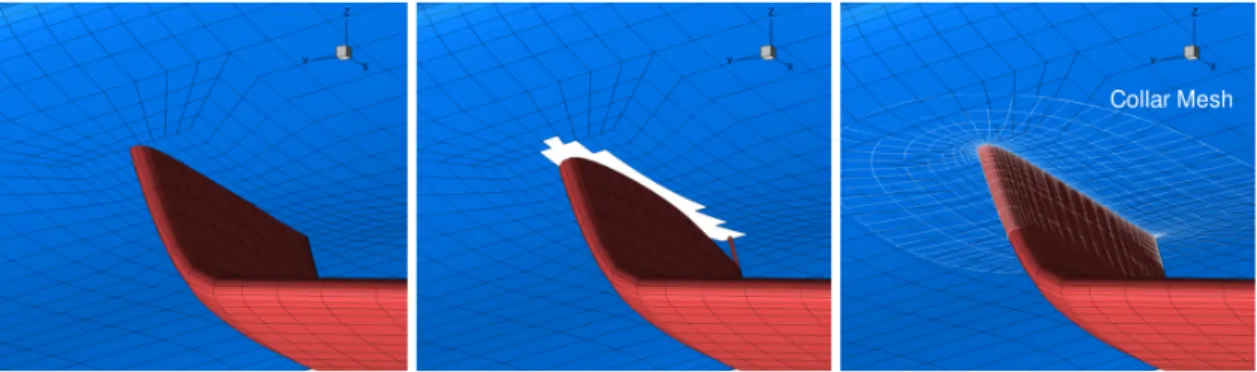
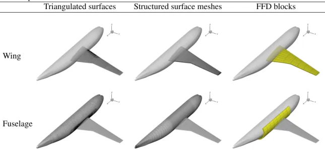
(a) Triangulated surfaces (b) Intersection computation

(c) Surface mesh marching (d) Volume mesh extrusion

Figure 2.1: Steps for generating collar mesh for a wing-fuselage junction. pySurf is re-sponsible for steps a–c. The mesh extrusion module used in step d (pyHyp) is covered in Sec.3.3.

2.2 Intersection computation

Once pySurf receives the triangulated surfaces, it has to compute intersections among them. The triangulated surface of a primary component may have tens of thousand elements.

(36)

Applying triangle-triangle intersection algorithms directly to all possible triangle pairs is costly. Therefore, the intersection computation in pySurf is performed in three steps to avoid unnecessary triangle-triangle intersection verification. The first two steps filter which triangles are likely to intersect by using methods based on Cartesian bounding boxes and digital tree searches, and we only use the triangle-triangle intersection algorithm in the third step.

Here we describe the steps to compute intersections between two components (for in-stance, component A and component B), since this process is repeated for every pair of primary components. First, we compute Cartesian bounding boxes for the two primary components, then we determine the intersection between these bounding boxes. Next we flag the triangles from both components that belong to the bounding box intersection re-gion. This step is relatively quick since we just need to compare maximum and minimum values of nodal coordinates against the Cartesian box bounds to flag the triangles.

In the second step, we take the flagged triangles of the component that has fewer flagged triangles (for example, component A) and build an alternating digital tree (ADT) [62] to minimize the tree complexity. This tree structure groups discrete elements based on their spatial location so we can efficiently find which pairs of elements are likely to intersect. We then take the bounding boxes of every flagged triangle of component B and perform ADT searches to find which flagged triangles from component A are close to it. At the end of this step, every flagged triangle of component B has a corresponding list of triangles from component A for the intersection search.

The third step consists of using fast pairwise triangle-triangle intersection algorithms [63] on the candidate elements given by the ADT searches to identify the two points that deter-mine intersection line between pair of triangles. We then concatenate the lines given by the pairwise triangle-triangle intersections to determine the entire intersection curve.

An arbitrary number of primary components can be intersected using this method. Each pairwise component intersection may have multiple intersection curves that could be se-lected as possible starting curves for the collar mesh generation detailed in the next section. We also added features dedicated to manipulating these intersection curves, such as merging, splitting, and remeshing, so that the user can accurately control the topology and the number of nodes describing the intersection, since this curve is the starting point for the hyperbolic surface marching. The number of nodes distributed along the intersection curve remains the same throughout the optimization to keep the same number of nodes in the CFD mesh.

(37)

2.3 Hyperbolic surface mesh generation

Having identified the intersection curves, we can now use hyperbolic mesh-marching algo-rithms [37] to produce the surface collar meshes. This type of mesh generation algorithm starts from a baseline curve and then uses a marching scheme to generate the next layer of the surface mesh. This process is repeated until the desired number of layers and mesh extension is reached. One advantage of hyperbolic marching schemes over other mesh generation methods (such as transfinite interpolation [64]) is that they do not require the outer boundary of the mesh domain to be defined, making the process easier to automate, especially for collar meshes.

We project every new layer of nodes onto the triangulated surfaces before the generation of the next layer to ensure consistency with the underlying geometry. For the projection step, finding the nearest surface triangle by brute force would not be tractable, especially when we must regenerate the mesh for each optimization iteration. Thus, we use the ADT algorithm once again to accelerate the search process. The ADT searches provide the closest surface elements to a given point, then we only need to compare projections on those filtered elements to find the nearest projection of the node onto the triangulated surface.

We added features to the standard hyperbolic marching scheme to improve control over the mesh generation, as discussed in AppendixA. For instance, the user can choose to pre-serve special surface features, such as trailing edge corners, as the surface mesh is marched. First we create a discrete representation of these curves using line segments. Then, we iden-tify which node from the baseline curve is closest to the guide curve segments and then we project this node onto the guide curve. In addition, we locally modify the marching equa-tions for this node so that it marches in a direction tangent to the guide curve. This process is repeated for every new layer of the marched mesh.

We also added a feature to preserve the relative node spacings from the baseline curve throughout the entire mesh. This feature works as follows: After every new layer is gener-ated, we redistribute the nodes of this new layer using the same relative arc-lengths of the nodes in the baseline curve. This redistribution is important when generating meshes near trailing edges, since the artificial dissipation associated with the marching scheme smooths the node intervals near the trailing edge despite the local high refinement of the baseline curve. Once the redistributed nodes are computed, we project them to the reference surface to ensure the consistency between the mesh and the surface representation.

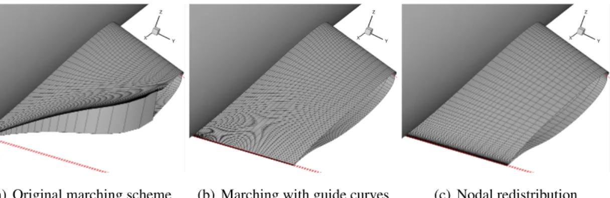
A comparison of meshes generated with and without these geometry-preserving options is shown in Fig 2.2. In Fig 2.2a, we simply extrude the mesh without considering any geometric features. In Fig 2.2b, we set the upper and lower edges of the blunt trailing

(38)

edge as guide curves. This forces the nearest point of the extruded mesh layer to coincide with the guide curve, which preserves the edge geometry. However, the bunched spacing at the leading and trailing edges dissipates as we march away from the intersection curve. Fig2.2c shows the effect of preserving the relative node spacing, what produces a surface mesh better suitable for CFD.

(a) Original marching scheme (b) Marching with guide curves (c) Nodal redistribution Figure 2.2: Additional features implemented in the collar marching scheme to improve mesh quality for CFD analyses.

2.4 Automatic differentiation

We need to efficiently compute derivatives of the objective and constraints to enable ef-fective gradient-based aerodynamic shape optimization. We apply the reverse mode AD

throughout the entire analysis chain for this purpose, what we discuss in detail in Sec.3.7. Therefore, pySurf also uses the sameADmethod to internally backpropagate partial deriva-tives.

Figure2.3outlines the notation used in this work to represent AD versions of a generic subroutineF that receives a vector of inputsX = [x1 x2 . . . xn]T and outputs the vector Y = [y1 y2 . . . ym]T, without loss of generality, since we always can concatenate multiple inputs and outputs in a single vector. In this figure,F˙ represents the forward AD version of the subroutineF, whileF represents the reverse AD version.

F X Y Original Function ˙ F X Y ˙ X Y˙ Forward Mode AD F X Y Y X Reverse Mode AD

(39)

The forward AD code propagates derivative seeds from inputs (X) to outputs (˙ Y), while˙ the reverse AD code propagates derivatives from outputs (Y) to inputs (X). The derivative seeds can be correlated with the following expressions [65]:

Original Function Forward Mode AD Reverse Mode AD

Y =F (X) Y˙ =J·X˙ X=JT _·_Y (2.1)

whereJis the Jacobian matrix correlating inputs and outputs of the subroutineF:

J = ∂Y ∂X =           ∂y1 ∂x1 ∂y1 ∂x2 · · · ∂y1 ∂xn ∂y2 ∂x1 ∂y2 ∂x2 · · · ∂y2 ∂xn .. . ... . .. ... ∂ym ∂x1 ∂ym ∂x2 · · · ∂ym ∂xn           . (2.2)

In Sec.2.2we mentioned that pySurf has several tools to control the intersection curves, such as merging multiple curves to create a new one, splitting curves based on sharp corners or intersections, and redistributing nodes along the curve to refine more important regions. During forward execution, pySurf stores all the intermediary steps required by the user to generate the appropriate curve for hyperbolic marching, then it uses the same steps, but in reverse order, to perform the reverse propagation of derivatives.

The automatically differentiated code for pySurf is generated using the Tapenade AD tool [65], but we have to selectively alter the differentiation process in each pySurf module to get an efficient final code. The next sections provide detailed explanation regarding these exceptions.

2.4.1 Projection subroutine

One of the steps of hyperbolic surface marching routine is the projection of the newly-generated points back to the reference triangulated surface. The initial step of the projec-tion algorithm consists of an ADT search to find the triangulated surface elements that are closest to the point to be projected. Then, we run the point-triangle projection algorithm on those candidate triangles and take the closest projected point. This point-to-triangle projection subroutine can be algorithmically described as:

(40)

whereFprojrepresents the projection routine,X0are the Cartesian coordinates of the point to be projected,XA,XB, andXC are coordinates of the three nodes from the triangle that will receive the projection, and Xproj is the projected point. We use the same projection subroutine to also compute the surface normal vectornprojof the triangle, since this vector is used by the hyperbolic mesh marching subroutine to determine the marching direction.

During the forward execution of the projection code, we store the triangles that receive the projections, so that we do not have to repeat the ADT searches during the reverse propagation of derivatives. Therefore, we only need to differentiate the point-to-triangle projection routine. The reverse-differentiated version of Eq. (2.3) is:

δX0, δXA, δXB, δXC = Fproj X0,XA,XB,XC,Xproj,nproj,Xproj,nproj

, (2.4) where the bars represents reverse derivative seeds, and the δ represents variations of the reverse derivative seeds that should be accumulated, since each triangle node may get con-tributions from multiple projections. That is:

X0 ←X0+δX0 XA←XA+δXA XB ←XB+δXB XC ←XC +δXC

(2.5)

2.4.2 Hyperbolic surface marching

The hyperbolic surface mesh marching generates the surface mesh layer-by-layer. LetRj−1 be a vector with3ni elements representing the Cartesian coordinates of theninodes of the layerj ₋1of the surface mesh. The nodal coordinates of the next layer are given by:

Rj =Rj−1+ ∆Rj, (2.6)

where the displacement∆Rj is obtained via the solution of a linear system defined by the discretized hyperbolic equations, as introduced in AppendixA:

Kj ·∆Rj =Fj. (2.7)

A dedicated routine computes the matrixKjand the right-hand side vectorFjbased on the nodal coordinates of the(j −1)-th layer (Rj−1) and on the normals of the underlying

triangulated surface at the projections of each node (nj−1):

Kj,Fj = Fhyp(Rj−1,nj−1) (2.8) During the reverse execution of the code, we initially have the derivative seeds of the