Modification of flow structures associated with broadband trailing edge noise

2016

Modification of flow structures associated with

broadband trailing edge noise

Hephzibah Clemons

Iowa State University

Follow this and additional works at:https://lib.dr.iastate.edu/etd Part of theAerospace Engineering Commons

This Dissertation is brought to you for free and open access by the Iowa State University Capstones, Theses and Dissertations at Iowa State University Digital Repository. It has been accepted for inclusion in Graduate Theses and Dissertations by an authorized administrator of Iowa State University Digital Repository. For more information, please [email protected].

Recommended Citation

Clemons, Hephzibah, "Modification of flow structures associated with broadband trailing edge noise" (2016).Graduate Theses and Dissertations. 15116.

Modification of flow structures associated with broadband trailing edge noise

by

Hephzibah Clemons

A dissertation submitted to the graduate faculty in partial fulfillment of the requirements for the degree of

DOCTOR OF PHILOSOPHY

Major: Aerospace Engineering Program of Study Committee: Richard Wlezien, Major Professor

Alric Paul Rothmayer Hui Hu

Anupam Sharma Sivalingam Sritharan

Iowa State University Ames, Iowa

2016

TABLE OF CONTENTS Page LIST OF FIGURES ... iv LIST OF TABLES ... x NOMENCLATURE ... xi ACKNOWLEDGMENTS ... xiv ABSTRACT………. ... xv CHAPTER 1 INTRODUCTION ... 1 1.1 Background ... 2

1.1.1 Trailing edge noise ... 2

1.1.2 Trailing edge noise reduction... 6

1.1.3 Flow instability ... 9

1.2 Objectives ... 11

CHAPTER 2 EXPERIMENT DESCRIPTION ... 12

2.1 Coordinate system ... 12

2.2 Hardware description ... 14

2.2.1 Airfoil model ... 14

2.2.2 Trailing edge modifiers ... 15

2.2.3 Low turbulence wind tunnel ... 20

2.2.4 Linear traverse system ... 21

2.2.5 Instrumentation ... 23

2.2.6 Probe vibration ... 25

2.3 Hot-wire measurements ... 26

2.3.1 Calibration procedure ... 26

2.3.2 Boundary layer profile measurement ... 29

2.3.3 Two-point velocity measurement ... 30

2.4 Data analysis ... 34

2.5 Turbulent boundary layer development ... 36

CHAPTER 3 RESULTS ... 41

3.1 Turbulent boundary layer near the trailing edge at α = 0º ... 41

3.1.2 Contour correlation data with respect to structures in Ot and It ... 44

3.1.3 Streamwise correlation of structures in Ot and It ... 47

3.2 Reference trailing edge configuration at α = 5º ... 49

3.2.1 Spanwise correlation of structures in the turbulent wake near the trailing edge ... 50

3.2.2 Contour correlation data with respect to structures in Ot, It and Ib ... 52

3.2.3 Streamwise correlation of structures in Ot, It and Ib ... 56

3.3 Effect of serrations on boundary layer development and flow structures near the trailing edge ... 57

3.4 Effect of trailing edge thickness on flow structures... 63

3.5 Effect of length of a serrated trailing edge on flow structures ... 67

3.6 Effect of width of a serrated trailing edge on flow structures... 76

CHAPTER 4 SUMMARY AND CONCLUSIONS ... 86

4.1 Summary ... 86

4.2 Conclusions ... 92

4.2 Future work ... 93

REFERENCES ... 94

APPENDIX A FIGURES ... 99

LIST OF FIGURES

Page

Figure 1(a) Illustration of trailing edge noise and its directivity pattern ... 3

Figure 1(b) Turbulent flow over an airfoil with a serrated trailing edge. Picture taken from Howe (“Aerodynamic noise of”) ... 6

Figure 2 Coordinate system ... 13

Figure 3 Airfoil model mounted in the test section ... 14

Figure 4 Blunt thickness modifier ... 15

Figure 5 Flat extended TE modifier F1 attached to Sh ... 16

Figure 6(a) Sketch of serrated TE modifier attached to Sh ... 17

Figure 6(b) Serrated TE as mounted in the test section ... 17

Figure 7 Effective serration ... 17

Figure 8 Dimensions of serrated TE modifiers ... 18

Figure 9 Low turbulence wind tunnel ... 21

Figure 10 Linear traverse system mounted in the test section ... 23

Figure 11 Accelerometer mounted on probe holder ... 25

Figure 12 Minimization of probe vibration ... 26

Figure 13 Calibration of hot-wire ... 29

Figure 14 Minimum separation between S and T ... 32

Figure 15 Derivatives of mean velocity with respect to voltage ... 34

Figure 16 Optimization of Reynold’s number at x/C = 0.5 ... 37

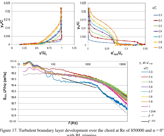
Figure 17 Turbulent boundary layer development over the chord at Re of 850000 and α = 0° with BL tripping ... 38

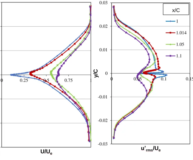
Figure 18(b) Turbulent boundary layer development in wall units ... 39 Figure 19 Turbulent wake development at Re of 850000 and α = 0°

with BL tripping ... 40 Figure 20 Three regions of interest in the turbulent boundary layer from

spanwise correlation data at x/C = 0.986. α = 0° ... 43 Figure 21 Three regions of interest shown in the TBL profile at

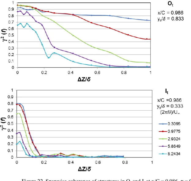
x/C = 0.986, 1. α = 0°... 43 Figure 22 Spanwise coherence of structures in Ot and It at x/C = 0.986.

α = 0° ... 44 Figure 23(a) Evolution of structures in Ot along the spanwise plane. S is

located at x/C = 0.986 and Δt = 0.00016 s. α = 0° ... 45 Figure 23(b) Evolution of structures in It along the spanwise plane. S is

located at x/C = 0.986 and Δt = 0.00016 s. α = 0° ... 45 Figure 23(c) Evolution of structures in Ot along the streamwise plane. S is

located at x/C = 0.986 and Δt = 0.00016 s. α = 0° ... 46 Figure 23(d) Evolution of structures in It along the streamwise plane. S is

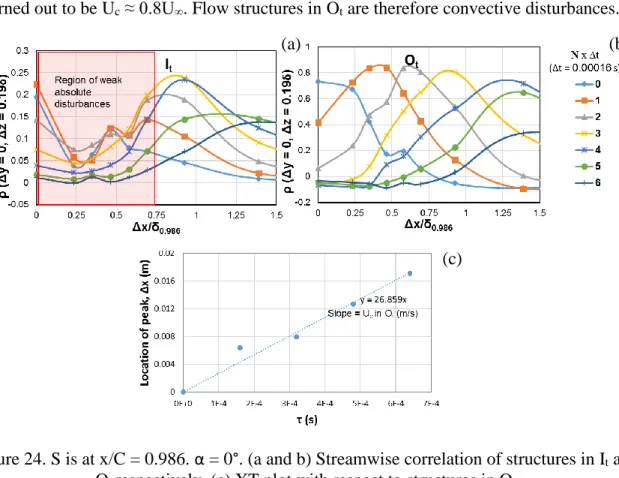
located at x/C = 0.986 and Δt = 0.00016 s. α = 0° ... 46 Figure 24(a) Streamwise correlation of structures in It.

S is at x/C = 0.986. α = 0° ... 48 Figure 24(b) Streamwise correlation of structures in Ot.

S is at x/C = 0.986. α = 0° ... 48 Figure 24(c) XT plot with respect to structures in Ot. S is at x/C = 0.986.

α = 0° ... 48 Figure 25(a) Wake profiles for Sh and B at x/C = 1, α = 5° ... 50 Figure 25(b) Normalized power spectral densities at Ib (pressure side) and It

(suction side) for Sh and B at x/C = 1, α = 5° ... 50 Figure 26 Regions of interest in the turbulent boundary layer (wake) from

spanwise correlation data at x/C = 1, α = 5° ... 50 Figure 27(a) Evolution of structures in Ot along the spanwise plane. S is

Figure 27(b) Evolution of structures in It along the spanwise plane. S is

located at x/C = 1 and Δt = 0.00016 s. α = 5° ... 53 Figure 27(c) Evolution of structures in Ib along the spanwise plane. S is

located at x/C = 1 and Δt = 0.00016 s. α = 5° ... 54 Figure 27(d) Evolution of structures in Ot along the streamwise plane. S is

located at x/C = 1 and Δt = 0.00016 s. α = 5° ... 54 Figure 27(e) Evolution of structures in It along the streamwise plane. S is

located at x/C = 1 and Δt = 0.00016 s. α = 5° ... 55 Figure 27(f) Evolution of structures in Ib along the streamwise plane. S is

located at x/C = 1 and Δt = 0.00016 s. α = 5° ... 55 Figure 28 Streamwise correlation of structures in Ot, It and Ib.

S is at x/C = 1. α = 5° ... 56 Figure 29 Turbulent boundary layer and wake development near the serration

L2W4 ... 58 Figure 30(a) Evolution of structures in Ot along the spanwise plane. S is

located at the root and Δt = 0.00016 s. ... 60 Figure 30(b) Evolution of structures in It along the spanwise plane. S is

located at the root and Δt = 0.00016 s. ... 60 Figure 30(c) Evolution of structures in Ot along the streamwise plane. S is

located at the root and Δt = 0.00016 s. ... 61 Figure 30(d) Evolution of structures in It along the streamwise plane. S is

located at the root and Δt = 0.00016 s. ... 61 Figure 31(a) Evolution of structures in It along the spanwise plane. S is

located at rs-tip and Δt = 0.00016 s. ... 62

Figure 31(b) Evolution of structures in It along the streamwise plane. S is

located at rs-tip and Δt = 0.00016 s. ... 62

Figure 32 Wake profiles measured at flat trailing edges of various

thicknesses ... 64 Figure 33 Evolution of structures in It near the trailing edge in the streamwise

Figure 34 Effect of trailing edge thickness on structures in It near the

trailing edge ... 66 Figure 35 Spanwise correlation of structures in It and Ot at trailing edges of

flat edged configurations... 67 Figure 36 Wake profiles measured at rs-tip of serrations of different lengths ... 68

Figure 37(a) Effect of length of serrations on convective speeds of structures in It

near the root ... 69 Figure 37(b) Effect of length of serrations on convective speeds of structures in It

near rs-tip ... 70

Figure 37(c) Effect of length of serrations on convective speeds of structures in It

near the tip... 70 Figure 38 Difference in convective speeds of structures in It at rs-tip and tip

positions for serrations of different lengths ... 71 Figure 39 Evolution of structures in the streamwise direction in It near the tip,

rs-tip of L3W1 and trailing edge of B ... 72

Figure 40 Evolution of structures in the spanwise direction in Ot near rs-tip

of L1W2, L3W1 and trailing edge of B ... 73 Figure 41(a) Spanwise correlation and half width of structures in It and Ot at the

root (varying 2h) ... 74 Figure 41(b) Spanwise correlation and half width of structures in It and Ot at the

rs-tip position (varying 2h) ... 74

Figure 41(c) Spanwise correlation and half width of structures in It and Ot at the

tip (varying 2h) ... 75 Figure 42 Wake profiles measured at rs-tip of serrations of different widths ... 77

Figure 43(a) Effect of width of serrations on convective speeds of structures in It

near the root ... 78 Figure 43(b) Effect of width of serrations on convective speeds of structures in It

near the rs-tip position ... 78

Figure 43(c) Effect of width of serrations on convective speeds of structures in It

Figure 44 Difference in convective speeds of structures in It at rs-tip

and tip positions for serrations of different widths ... 80 Figure 45(a) Spanwise correlation and half width of structures in It and Ot at

the root (varying λ) ... 81 Figure 45(b) Spanwise correlation and half width of structures in It and Ot at

the rs-tip position (varying λ) ... 81

Figure 45(c) Spanwise correlation and half width of structures in It and Ot at

the tip (varying λ) ... 82 Figure 46(a) Half width of structures in Ot at the rs-tip and tip positions

respectively ... 84 Figure 46(b) Difference in convective speeds of structures in It

at the rs-tip and tip positions ... 84

Figure a1 Streamwise correlation of structures in Ot.

S is at x/C = 1, Δt = 0.00016 s, α = 0° ... 99 Figure a2 Streamwise correlation of structures in It.

S is at x/C = 1, Δt = 0.00016 s, α = 0° ... 100 Figure a3 Spanwise correlation of structures in Ot and It.

S is at x/C = 1, Δt = 0.00016 s, α = 0° ... 101 Figure a4 XT plot of structures in Ot at trailing edge of flat edged

configurations ... 102 Figure a5 XT plot of structures in Ot at rs-tip of serrations

of different lengths ... 102 Figure a6 XT plot of structures in Ot at rs-tip, tip of serrations

of different lengths ... 104 Figure a7 XT plot of structures in Ot at rs-tip of serrations

of different widths ... 103 Figure a8 XT plot of structures in Ot at tip of serrations

of different widths ... 104 Figure a9(a) Boundary layer profiles at root of all serrated TE configurations ... 104 Figure a9(b) Wake profiles at rs-tip of all serrated TE configurations ... 105

Figure a9(c) Wake profiles at tip of all serrated TE configurations ... 105 Figure a10(a) Convective speed of structures in It (region 1 and 2) near root for

all serrated TE configurations compared with

flat TE configurations ... 106 Figure a10(b) Convective speed of structures in It (region 1 and 2) near rs-tip for

all serrated TE configurations compared with

flat TE configurations ... 106 Figure a10(c) Convective speed of structures in It (region 1 and 2) near tip for

all serrated TE configurations compared with

flat TE configurations ... 106 Figure a11(a) Half width of structures in Ot near root for all serrated

TE configurations... 107 Figure a11(b) Half width of structures in It near rs-tip for all serrated

TE configurations... 107 Figure a11(c) Half width of structures in It near tip for all serrated

LIST OF TABLES

Page Table 1 List of TE modifiers ... 19

NOMENCLATURE

BL boundary layer

TBL turbulent boundary layer TE trailing edge

S, T stationary and traversing hot-wires respectively

X, Y, Z global orthogonal coordinate system. Streamwise, normal and span- wise directions respectively

α angle of attack x, y, z variables in (X, Y, Z) respectively

Δx, Δy, Δz distance between S and T in (X, Y, Z) respectively

ys distance from the surface of the airfoil along the y-direction at a given

x/C

U unsteady velocity along the x-direction U mean velocity along the x-direction

u’ fluctuating component of velocity along the x-direction u’rms root mean square of u’

U∞ free-stream velocity along x-direction

Uc eddy convective velocity along x-direction

u’max maximum u’ in the local boundary layer

Ue Velocity along the x-direction at the edge of the local boundary layer

δ, δb local boundary layer thickness on the suction and pressure side

δ*_{, δ}*

b local displacement thickness of the boundary layeron the suction and

pressure side respectively

θ local momentum thickness of the boundary layer

δ, δb suction and pressure side boundary layer thicknesses respectively at the

trailing edge of the reference airfoil at α of interest

δ0.986 boundary layer thickness on the suction side of the reference airfoil at

x/C = 0.986 at α of interest δ*_{, δ}*

b suction and pressure side boundary layer displacement thicknesses

respectively at the trailing edge at α of interest C chord length

M subsonic Mach number

t trailing edge thickness

2h length of a serration from root to tip measured along the x-direction

λ width of a serration - distance between two roots or tips measured along the z-direction

rs,ts root and tip z-positions respectively of serrations projected onto any y-z

plane

φ angle of serration - tan-1_(λ/4h)

ρ cross correlation coefficient γ2 _coherence

SSS ,STT auto-spectral densities of S and T respectively

STS cross-spectral density of S and T

τ time delay between signals from S and T

f frequency

k wave number

ACKNOWLEDGMENTS

First, I would like to thank God almighty without whom nothing good would be possible. All glory and honor be to him alone.

I am very deeply indebted to many people who have contributed to my work. I thank my major professor and mentor Prof. Richard Wlezien who has guided me patiently through this whole process for the last 5 years. He has been extremely supporting and has taught me so much more than just to do with my research. I am truly honored to have had him as my guide.

I would like to thank Dr. Rothmayer, Dr. Hu, Dr. Sharma and Dr. Sritharan for their valuable input to my research and for being on my committee. I also thank the department staff who made the last few years very memorable. Special thanks to our research team Lucas Clemons, Anil Jairam, Julie Bothell and Eli Shellabarger for all the help, day or night given to me in the laboratory. I also thank Edgardo Diaz and other undergraduates who helped with my research. In addition, I would like to thank the Department of Aerospace Engineering at Iowa State University for the wonderful experience and opportunities I have had.

My deepest gratitude goes to my parents, the inspiration for my doctoral program. I thank my sister and family for their prayers, my parents-in law for their support and all my family and friends for helping me complete my degree. Lastly and most importantly, I thank my husband, colleague and dear friend Lucas Clemons for standing through it all with me.

ABSTRACT

Trailing edge (TE) noise due to the interaction between a turbulent boundary layer (TBL) and an airfoil trailing edge is a major source of airfoil self-noise. This broadband noise source generates sound from a few 100 Hz well into the KHz range (~ 15,000 Hz). Wind turbine blades and other subsonic airfoils generate significant TE noise. Improvements such as serrations added to the trailing edge have shown to decrease the far-field noise generated without compromising the aerodynamic performance. A number of aeroacoustic TE noise theories have long been used as the basis for noise-reduction mechanisms. It is well known that they over-predict noise generation and reduction. Serrated trailing edges with different geometries are also known to decrease noise in certain frequency ranges and increase noise in others. In light of these discrepancies, recent work has been focused on understanding the flow mechanisms that cause noise and, by extension, the mechanisms that reduce noise.

In the present research, a NACA 0012 airfoil at a chord Reynold’s number of ~850,000 and Mach number of 0.1 was chosen as a baseline configuration to study broadband noise generating flow mechanisms near the trailing edge. The results from the airfoil with a modified blunt trailing edge and 5° angle of attack were used as the baseline. Hot-wire anemometry with two traversing hot-wires were used as the main sensor for unsteady velocity measurements. Spanwise and streamwise correlations were obtained at different depths in the fully turbulent BL near the trailing edge of the baseline configuration to characterize flow structures. From these data, two regions having weak absolute and convective disturbances in the streamwise direction were isolated: the inner log region and the outer region respectively.

Correlation and BL profile data near trailing edges of varied thicknesses were compared and it was found that a decrease in thickness and wake deficit near the trailing edge corresponded to an increase in the convective speed of flow structures in the inner region. Sharpness transitions an unsteady wake to an unsteady mixing layer. It has been experimentally proven by other studies that an increase in TE noise occurs with an increase in its thickness. This follows that the interaction of weak absolute disturbances in the inner region with the trailing edge could be a major mechanism of noise generation.

Various serrated TE modifiers whose dimensions λ and 2h (λ is the width between two tips or roots and 2h is the length of a serration from root to tip) were scaled to the TBL thickness at the trailing edge of the baseline configuration were used as flow modifiers. The serrations formed a three dimensional flow structure with different convection speeds along the span. The effect of increasing the length of serrations was to transition the inner region of the turbulent boundary layer near the serration from weak absolute to convective

disturbances and to decrease the spanwise correlation of flow structures near the tip. Results suggest that for a given serration width there exists a maximum length that corresponds to the greatest decrease in TE noise. This maximum length has been independently verified by other studies. It was also found that for a given large serration length there exists a minimum width that corresponds to an optimum convective speed of flow structures in the inner region near the serration. Evidence suggests that this width organizes the three dimensional flow structure most desirably to obtain the highest spanwise decay rate of flow-structures near the tip resulting in the maximum reduction of TE noise. Thus, the complex interaction of flow structures near the serration sheds light into the noise reduction mechanism of serrated trailing edges.

CHAPTER 1 INTRODUCTION

Airfoil self-noise is caused by the interaction of an airfoil with the turbulence

produced in its boundary layer and near wake. Turbulent boundary layer–trailing edge (TBL-TE) interaction noise is one of the major sources of airfoil self-noise and has a unique cardioid shaped directivity. It scales effectively as M5_{. It is broadband in nature and exists}

from a few 100 Hz well into the KHz range (~ 15,000 Hz). Wind turbine blades and other subsonic airfoils generate significant TE noise that can be a source of discomfort to those nearby. As the name suggests, it is very dependent on the property of the trailing edge and the turbulent boundary layer in its vicinity. Hence, changes made to either one of these components should affect TE noise. Improvements such as serrations added to the trailing edge have shown to decrease the far-field noise generated without compromising the aerodynamic performance (Tanner, M (1972), Nedić, J and Vassilicos, J. C (2015)) A number of aeroacoustic TE noise theories have long been used as the basis for noise-reduction mechanisms. It is well known that they over-predict noise generation and

reduction. Serrated trailing edges with different geometries are also known to decrease noise in certain frequency ranges and increase noise in others. These discrepancies suggest the need to further understand how the flat and serrated trailing edges interact with the turbulent boundary layer nearby. Recent work has been focused on understanding these flow

mechanisms that cause noise and, by extension, the mechanisms that reduce noise. This could potentially help in designing better systems for TE noise control.

1.1 Background

1.1.1 Trailing edge noise

Aerodynamic noise associated with an airfoil can be classified into inflow turbulence noise and airfoil self-noise. Inflow turbulence noise is caused by the interaction of turbulence in the atmosphere with the leading edge. The unsteady lift generates a dipole like source and the noise it produces is in the broadband low frequency range. Airfoil self-noise is due to the interaction between an airfoil and the turbulence produced in its own boundary layer near the wake. It is the total noise produced when an airfoil encounters laminar flow. The interest in airfoil self-noise is many fold. It occurs commonly as helicopter rotor, wind turbine and airframe noise. It can be further classified into five self-noise mechanisms (Brooks, T. F et al. (1989)): turbulent boundary trailing edge noise (TBL-TE), laminar boundary layer-vortex shedding noise (LBL-VS), separation stall noise, tip layer-vortex formation noise and trailing edge bluntness-vortex shedding noise. Of these, TBL-TE was found to be the hardest to predict and control. It is a major contributor to broadband noise from the low to high frequency range and is of particular interest in low-speed flow regimes like a wind turbine. Many studies for the past few decades have been dedicated to the study of trailing edge noise. Figure 1 illustrates TE noise: the scattering of pressure waves caused by the interaction of the trailing edge with turbulent eddies in the boundary layer. The cardioid shaped

directivity pattern of TE noise is shown beside. In a cambered airfoil or an airfoil at a finite angle of attack, the far-field tonal noise is usually associated with the high energy eddies on the pressure side while the turbulence on the suction side contributes solely to broadband noise.

Figure 1(a). Illustration of trailing edge noise and its directivity pattern

Lighthill (1952, 1954) in his theory of aerodynamic sound, modelled the problem of sound generation by turbulence using an exact analogy where sound was radiated by a volume distribution of acoustic quadrupoles in an ideal acoustic medium. The strength of the quadrupoles in Lighthill’s stress tensor used in his theory are the unsteady components of the Reynold’s stress at low Mach numbers. Curle (1955) showed how the presence of boundary surfaces could be accounted for by adding dipole and monopole sources. A dimensional analysis of the equations showed that the intensity of sound generated by free turbulence (quadrupoles) scales as the eighth power of a typical flow velocity while that induced by unsteady surface forces (dipoles) scales as velocity to the power six. Some of the earliest studies on trailing edge noise were performed by Ffowcs Williams and Hall (1970), Chase (1972) and Amiet (1975 and 1976). Ffowcs Williams and Hall (1970) stated that it was necessary to consider the details of the potential field in the vicinity of a sharp edge of a body that acts as a scattering center. In such a case, dimensional analysis showed that the sound generated is dominated by edge scattering and the resulting noise scales more effectively than a quadrupole or a dipole. The intensity scales as typical flow velocity (Uc) to the power

five and is given by 〈𝑝2〉 ∝ 𝜌₀2U_c5(𝐿𝑙𝐷̅ _𝑐 0𝑟2

⁄ ), where p is the far-field acoustic pressure, 𝜌₀ is the medium density, 𝑐₀ is the speed of sound, r is the distance from the trailing edge to the

observer, 𝐷̅ is a directivity constant that equals 1 for observers normal to the surface from the trailing edge, L is the spanwise trailing edge length wetted by the flow and l is a

characteristic turbulence correlation scale. The effect of an eddy on trailing edge noise was calculated to be substantially higher when near the edge, within a hydrodynamic wavelength. He also showed the occurrence of cardioid shape directivity (sin2(θ/2), θ is the angle made about the TE as shown in figure 1) associated with trailing edge noise. This particular U_c5 scaling was independently observed in other studies performed by Chase (1972), Howe (1978) and in acoustic experiments performed by Brooks and Hodgson (1981) among others. Chase (1972) related the far-field pressure spectrum to hydrodynamic pressure fluctuations on or near the trailing edge in the presence of a turbulent wall jet. He used measurable properties on the boundary layer upstream of the trailing edge in his theory. He also assumed that the turbulent eddy convected past the trailing edge without interacting with it

(evanescent wave). Amiet (1975, 1976) theoretically related the far-field acoustic spectrum to the spanwise correlation length of vertical velocity fluctuation and surface pressure spectrum near the trailing edge. These theories were compared to experimental results and the results did not match as expected. They were limited by the right use of turbulence spectrum, surface pressure spectrum and so on. The theories themselves made considerable assumptions like the evanescent wave mentioned above, absence of mean flow, average value of eddy convective velocity and so on.

Howe (1978) formulated his theory on trailing edge noise. He made modifications from the earlier theories: he accounted for varying convective speeds of turbulent eddies with respect to vertical distance from the trailing edge (Uc(y)), forward flight motion and lack of

showed the predicted noise is proportional to turbulence wetting length L, spanwise

correlation length of eddies l and eddy convection velocity Uc to the power five. They agreed

with previous findings. The most important contribution was the application of the Kutta condition at the trailing edge to account for finite pressure and velocities at trailing edge (as opposed to the evanescent wave theory). His theory showed that the application of Kutta condition under-predicted the far-field noise generated by about 10 dB when compared to results without the use of Kutta condition. Howe explained this discrepancy by the use of a correction factor (1- (W/Uc(y))-2, where, W is the speed of shed vortex in the near wake in

the y = 0 plane and takes values from 0 to Uc(y) based on the problem being analyzed. Other

authors (Brooks, T. F and Hodgson, T. H (1981), Rienstra, S. W (1981)) went on to suggest that the truth in practicality lies somewhere in between, very likely through the application of viscosity in the closer regions to the trailing edge. They did not observe any vortex shedding as a result of the Kutta condition in their experiments (or theory). Lutz et al. (2007) and Kamruzzaman, M et al. (2011) showed the importance of using correlation length of vertical velocity fluctuating components in the vertical direction and mean shear of the turbulent boundary layer while theoretically predicting wall pressure fluctuations that inevitably contribute to far-field noise as stated by previous authors. All the above work is limited to high frequency trailing edge noise where the associated wavelengths are considerably smaller than the chord length of the airfoil. From this review, the need to further explore the effect of turbulence and its interaction with the trailing edge is apparent.

In recent years, many aeroacoustic computational studies have been performed on specific problems, example: computational aeroacoustic analysis of a high lift configuration by Singer et al. (2000) and its corresponding experimental study by Choudhari et al. (2002),

convective effects and the role of quadrupole sources for airfoil aeroacoustics by Wolf et al. (2012). The results of vortex shedding by Singer were compared with experiments performed in their group and were found to be agreement. Few results from the computations on a NACA 0012 airfoil performed by Wolf were in agreement with experimental data by Brooks (1981,1989). Discrepancies were still observed at complex flow configurations.

1.1.2 Trailing edge noise reduction

In light of the trailing edge noise problem, many studies have been performed to mitigate it. Some of the earliest ones stem from Howe’s theoretical work on serrated trailing edges (1991) in a low Mach number flow. He suggested the use of passive devices: serrated trailing edges of serration angle (figure 1(b)) φ < 45º would reduce noise by up to 8 dB at high frequencies (fδ/U∞ > 0.16, fh/U∞ >> 1, where δ is the boundary layer thickness of the

trailing edge and 2h is the length of the serration as shown in figure 1(b)).

Figure 1(b). Turbulent flow over an airfoil with a serrated trailing edge. Picture taken from Howe (“Aerodynamic noise of”)

φ U

Howe explained that as noise is understood to be directly proportional to the effective wetting length of convective eddies arriving normal to the trailing edge, any method to reduce the effective wetting length could potentially reduce noise. He over predicted noise reduction and this was experimentally shown by many authors including Gruber et al. (2010, 2011). Gruber showed that at some frequency fδ/U∞ ≈ 1, the noise generated by sawtooth

serrations of all dimensions (2h and λ – figure 1(b)) increases. He also showed that serrations are most efficient in the length range 1 < 2h/δ ≤ 4. In addition, noise reduction improves when λ decreases. He attributed the increase in noise to jets forming in between the serrations. He observed that where noise was reduced, it occurred over low to mid frequencies by 1 to 7 dB respectively. Noise increase of over 3 dB occurred at high frequencies. He could not establish a trend between h and λ even though he observed that they depended on each other with respect to noise reduction. Few others showed that the same serration dimension that worked at a given frequency range at high Reynold’s numbers caused an increase in noise at low Reynold’s numbers signifying a dependence of

effectiveness of serrations on flow dynamics near the trailing edge. It has also been shown that serrations do not affect the aerodynamic performance of the airfoil, in fact, they can improve it (Tanner, M (1972), Nedić, J and Vassilicos, J. C (2015)).

Oerlemans et al. (2001) showed that modifying the shape of the airfoil and adding serrations could reduce noise by 4 to 7 dB. Dassen et al. (1996) showed that misaligned teeth of ≈ 15º with respect to the chord plane increases noise. Finez et al. (2010) used

polypropylene fibers at the trailing edge and noticed a reduction of ≈ 3 dB noise. This was attributed to the coherent decay of structures in the spanwise and transverse direction of the trailing edge. Herr (2005, 2007) also experimentally studied flexible and rigid brushes/combs

as trailing edge noise treatments and found noise reduction of 2 to 10 dB over a wide

frequency range. He attributed this to viscous damping of turbulent flow pressure amplitudes in the comb area. In general, it was observed that noise reduction depended on length, width, spacing and flexibility of the brushes through their effect on local flow structures near the trailing edge.

Khorrami and Choudhari (2003) computationally applied passive porous treatments to slat trailing edge noise. They found potential reduction of about 20 dB across frequency regions of interest accompanied by a secondary effect of an upward shift in shedding

frequency to a frequency band of reduced auditory sensitivity in full-scale applications. Wolf et al. (2015) used active noise reducers (wall normal suction) to alter the boundary layer characteristics responsible for trailing edge noise. He showed that steady suction had a positive effect on the trailing edge noise (reduction by 3.5 dB) by reducing boundary layer thickness and the integral length scales of eddies in the boundary layer. Jaworski and Peake (2013) mathematically studied the effect of porosity and elasticity of a scattering edge. They showed that it might be possible to reduce noise scattering from a rigid edge from Uc5 to Uc6

and Uc7 respectively by the appropriate use of porosity and elasticity as in an owl’s wing.

Following this, Clark et al. (2014, 2015) tested passive bio-inspired rough surfaces and canopies to modify the turbulence features before they scatter into trailing edge noise. They had considerable success over a wide frequency range (10 dB attenuation) and dependence on modifier geometries is being studied. Again, an increase in noise at high frequencies was observed for a few TE treatments and could not be explained. These modifiers were a combination of rough surfaces, porous and flexible materials.

Much effort has been dedicated towards the progress of trailing edge noise reduction. The presence of turbulent features near the trailing edge and their interaction with the trailing edge, with or without the use of modifiers is the underlying problem behind most of this research and there is work yet to be done in this particular field of research. In this study, we make use of known sawtooth serrations to better understand some of these basic flow

problems involved in trailing edge noise.

1.1.3 Flow instability

In the course of this research, it was found that absolute and convective disturbances affect the nature of trailing edge noise to varying degrees. This section gives a brief

introduction to the concept of these two instabilities. Huerre and Monkewitz (1990) in their review of local and global instabilities in spatially developing flows explained the concepts of classical linear stability theory concerned with the development in space and time of infinitesimal perturbations around a basic parallel flow U(y; R) where R (example: Reynold’s number) is the sole control parameter that defines the character of U in the local x-position. Fluctuations are typically decomposed into elementary instability waves ϕ(y; k)e{i(kx - ωt)}

of

complex wave number k and complex frequency ω. ϕ(y; k) is shown in most cases to satisfy

an ordinary differential equation of Orr-Sommerfeld type. After enforcing boundary conditions, it leads to an eigenvalue problem where eigenfunctions ϕ(y; k) exist only if k, ω

satisfy a dispersion relation of the form given in equation 1.1.

D[k, ω; R] = 0 (1.1)

It is possible to ignore variations in the y-direction and consider the spatio-temporal evolution of instability waves in the (x, t)-plane without losing any of the important

characteristics of stability. A differential operator D[ -i(𝜕/𝜕x), i(𝜕/𝜕𝑡); R] in physical space (x, t) is associated with the dispersion relation (in spectral space) in equation 1.1 such that the fluctuations ψ(x,t) satisfy equation 1.2.

D[−𝑖_𝜕x𝜕 , 𝑖_𝜕t𝜕; 𝑅] ψ(x,t) = 0 (1.2) The impulse function G(x,t) (Green’s function) of the flow in question is given by equation 1.3.

D[−𝑖_𝜕x𝜕 , 𝑖_𝜕t𝜕 ; 𝑅] G(x,t) = δ(x)δ(t) (1.3) where δ is the Dirac delta function.

The basic flow is then said to be linearly stable if lim

t→∞G(x, t) = 0 along all rays x/t = constant, (1.4) and it is linearly unstable if

lim

t→∞G(x, t) = ∞ along at least one ray x/t = constant. (1.5) Among linearly unstable flows, the basic flow is convectively unstable if

lim

t→∞G(x, t) = 0 along the ray x/t = 0, (1.6) and it is absolutely unstable if

lim

t→∞G(x, t) = ∞ along the ray x/t = 0. (1.7) In general, convective disturbances vary in space and absolute disturbances vary in time. Given a parallel flow approximation, at a local streamwise station, if localized

disturbances spread upstream and downstream and affect the entire parallel flow, the velocity profile is said to be locally absolutely unstable. If the disturbances are swept away from the source, it is said to be locally convectively unstable. The implication of a locally absolute flow often is that it results in globally instability. The spatial evolution of unsteady flows that

are locally convectively unstable everywhere (example: mixing layers) is in large determined by the amplitude or frequency content of the excitation of the control. They are in essence “noise amplifiers”. On the other hand, shear flows with regions of absolute instabilities of sufficiently large size (example: bluff-body wake) behave as “oscillators” where fluid particles are advected downstream, but temporally growing global modes may be present. The evolution of vortices does not rely on spatial amplification of external perturbations but on the growth of initial disturbances in time.

1.2 Objective

The objective of this research is to understand the basic flow mechanism involved in the generation of broadband TE noise. Given the discrepancies between theories associated with TE noise, the goal is to find the common denominator flow physics that could better explain it. By contrasting the flow structures and their interaction with flat trailing edges with the flow structures and their interaction with known independently verified “good” and “bad” serrated trailing edge noise reducing modifiers, we want to investigate flow mechanisms that generate and reduce noise. Through this process, we intend to expand the design space for practical and effective trailing edge noise reducing modifiers.

CHAPTER 2

EXPERIMENT DESCRIPTION

A NACA 0012 airfoil was chosen for study because it is a simple airfoil and many aeroacoustic and experimental fluid studies have used it before. It has become a good standard for comparison in basic flow problems. Research by Brooks, T. F et.al (1989) and Brooks, T. F and Hodgson, T. H (1981) are a few well-known studies that have used the given airfoil in their experiments to measure and predict TE noise. In more recent years, Wolf, W. R et al. (2012) performed compressible large eddy simulations on a NACA 0012 airfoil with a rounded edge to study the effects of mean-flow and quadrupole sources on TE noise. This airfoil is optimally thick to provide a turbulent boundary layer at the trailing edge as often is the case in low speed airfoils (eg: wind turbines). It is a symmetric airfoil and therefore the broadband flow problem can be de-coupled from the tonal component at high Reynold’s numbers, for a sharp trailing edge and at zero degrees angle of attack. Knowledge of this broadband flow structure is used for the main part of this research where the

broadband flow structures modified near the trailing edge at α = 5° is explored. The turbulent boundary layer generated near the trailing edge at this angle of attack is optimal for this study as it can be compared to what happens in practicality.

2.1 Coordinate system

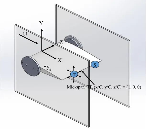
The schematic diagram of the orthogonal coordinate system used in this study is shown in figure 2.

Figure 2. Coordinate system

Figure 2 shows the airfoil model mounted to the side panels of the wind tunnel at α = 0°. The X-axis is along the streamwise direction. The Z–axis is in the spanwise direction and the Y-axis is in the normal direction. The mid-span of the trailing edge is taken as the point of reference at any angle of attack and takes the value (x/C, y/C, z/C) = (1, 0, 0). The distance from the surface of the airfoil measured along the y-direction is given by ys. In the wake, ys =

0 is the point that has the least streamwise velocity U. S and T are the stationary and traversing hot-wires respectively.

X

Y

Z

U

y

S

T

2.2 Hardware description 2.2.1 Airfoil model

The NACA 0012 airfoil model used has a chord length C = 18 in. The experimental setup was designed to run at a Reynolds number of ≈ 850000 and Mach number of 0.1. The airfoil model was machined out of one solid piece of RenShape 440, a medium-low density polyurethane board. It was sanded, painted and finally sanded again with a 2000 grit

sandpaper. The CNC machine used to machine the model has a tolerance of ≈ ± 0.0005 in. The trailing edge is rounded and has a radius of curvature of ≈ 0.025 in (t ≈ 0.05 in or

0.003C). To develop a turbulent boundary layer at the trailing edge, the boundary layer was tripped at 10% chord by a roughness of ≈ 0.0007C. The roughness consists of glass beads of size 60 grit (≈ 0.01 in) stuck to the model at 10% chord by a ¼ in, 0.002 in thick double sided adhesive tape. The glass beads were tightly packed and randomly distributed on the double sided adhesive. Figure 3 shows the airfoil model as mounted in the wind tunnel.

Figure 3. Airfoil model mounted in the test section

BL tripping at 0.1C Angle controller α_max = ±5°

A manual angle control attached to both the sides of the model and the test section was used to control the angle of attack of the incoming airflow with respect to the chord. The maximum angle that could be set with the controller is αmax = 5°. The airfoil was mounted

such that it could be rotated about 0.25C.

2.2.2 Trailing edge modifiers

All modifiers were rapid prototyped from UV cured VeroWhite+. They were attached to the airfoil with Mylar tape of thickness ≈ 0.002 in. A total of 12 TE modifiers were used. The first modifier was a bluntness or thickness modifier. Figure 4 schematically shows the blunt thickness modifier attached to the original “sharp” trailing edge - Sh. The resulting trailing edge was named as “blunt” trailing edge - B and was used as the reference

configuration at α = 5°. The reasons for these choices, names and the effect of the Mylar tape on the turbulent boundary layer are described later in the results section. The effective

thickness for the blunt trailing edge, taking the Mylar tape into account is t ≈ 0.09 in.

Figure 4. Blunt thickness modifier

For the purpose of our study, it is undesirable for the modification geometry and not the serrations to alter the flow structures near the trailing edge. For this reason, 2

modifications F1 and F2 were added to the original trailing edge. They differ from the serrations in that they do not have serrations (they are flat) and they extend the chord of the airfoil over ≈ 1.2 in. These modifiers followed the profile of the airfoil near the trailing edge but have different rounded TE thicknesses (t = 0.05 in and 0.16 in respectively). Figure 5

schematically shows the first of these flat extended trailing edges F1 attached to Sh. Mylar tape of thickness ≈ 0.002 in was used to attach the lip of modifiers to the suction and pressure sides of the original airfoil. F1 and F2 were also used to study the effect of TE thickness on the flow structures in the turbulent boundary layer near the trailing edge. The effect the lip of the modifier/ Mylar tape on the turbulent boundary layer is insignificant near the new

extended trailing edge (displaced downstream of the original TE) as are discussed later in the results.

Figure 5. Flat extended TE modifier F1 attached to Sh

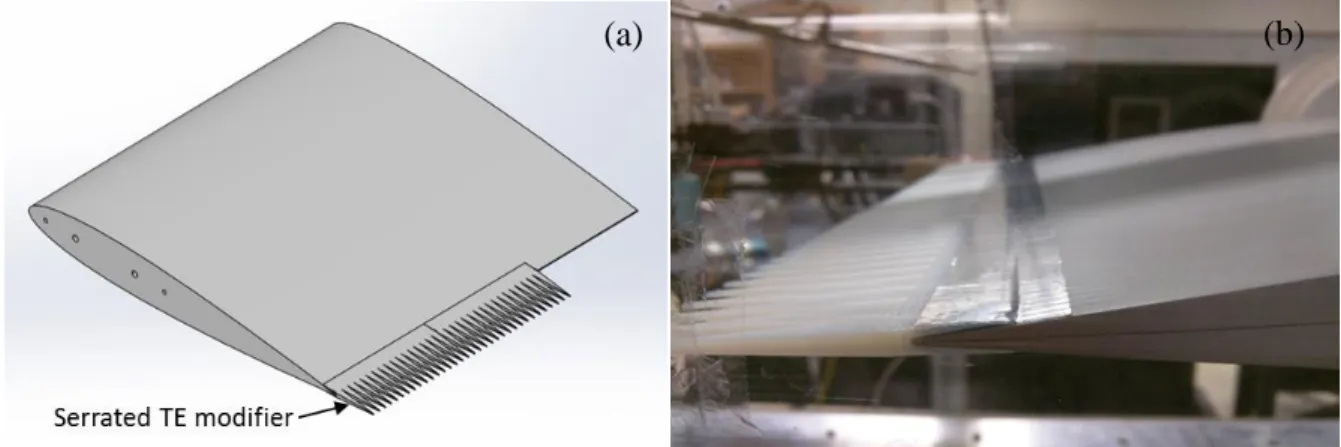
Nine serrated TE modifiers were used in this study. They were attached to the

original airfoil in the same way as F1 and F2, as described above. Figure 6(a) shows a sketch of a serrated TE modifier attached to the original airfoil and figure 6(b) shows the serrated trailing edge as mounted in the wind tunnel.

Figure 6. (a) Sketch of serrated TE modifier attached to Sh. (b) Serrated TE as mounted in the test section

Previous analytic and experimental work (Howe, M. S (1991) and Gruber, M et al. (2011)) show that serrations need to be scaled with respect to the boundary layer at the trailing edge for them to be effective at noise reduction. Figure 7 shows a schematic diagram of an effective serrated trailing edge with important notations that are used in this study.

Figure 7. Effective serration

Following this, the dimensions of the serrated TE modifiers used were scaled to the boundary layer thickness at the trailing edge of the reference configuration (B) at α = 5° (δ = 0.72 in) and are shown in figure 8. The findings from Gruber, M et al. (2011) and Howe, M. S (1991) were used as a reference to pick the dimensions of serrations. Gruber, M et al.

(2011) experimentally showed that a serration is most effective at 1 < 2h/δ ≤ 4 and for smaller values of λ. He could not establish a consistent trend between 2h and λ for effective noise reduction. In our study we picked a range of values of 2h (length) and λ (width) to reach our goals. Some of these serrations (example: L2W4) were shown to reduce noise by Gruber, M et al. (2011) while others (example: L1W1) are expected to be poor noise

reducers. Such a choice could make a comparison of the flow structures around the baseline TE configuration to those around serrations of “good” and “bad” serrated trailing edges meaningful i.e., they could point out the flow mechanism that actually helps in noise

reduction. Table 1 shows a list of all the modifiers used alongside their configuration names, relevant dimensions and color coding that will be used throughout this study.

Figure 8. Dimensions of serrated TE modifiers

0 0.5 1 1.5 2 2.5 3 3.5 4 4.5 5 0 1 2 3 4 5

2

h/

δ

λ/δ

Table 1. List of TE modifiers TE

configuration name

Pictographic representation and color code 2h/δ λ/δ t Tip/ TE (in) Root (in) Sh 0 ∞ 0.05 N/A B 0 ∞ ≈ 0.09 N/A F1 0 ∞ 0.05 N/A F2 0 ∞ 0.16 N/A L1W1 1.5 4.1 0.05 0.19 L1W2 1.4 0.5 0.05 0.19 L2W1 2.9 4.1 0.05 0.19 L2W2 2.9 2.1 0.05 0.19 L2W3 2.9 1.0 0.05 0.19

All serrations are drawn to scale:

Table 1. continued

L2W4 2.9 0.5 0.05 0.19

L2W5 2.8 0.2 0.05 0.19

L2P2 2.8 0.5 0.05 0.19

L3W1 4.3 0.5 0.05 0.19

All serrations are drawn to scale:

The configuration L2P2 was designed such that the plan-wise effective porosity of the serrated trailing edge would be 25% as opposed to the standard 50% porosity that all

triangular (sawtooth) serrated trailing edges will have.

2.2.3 Low turbulence wind tunnel

The experiment was performed in the low turbulence wind tunnel at the aerospace engineering department of Iowa State University. It is a closed loop wind tunnel with a test section– 60 in x 24 in x 18 in (length x height x width). A proportional integral controller connected to its cooling system regulates the temperature in the tunnel to an accuracy of ± 2.5 °C. A differential pressure transducer connected to entrance of the test section and the contraction section respectively measures the free-stream velocity (U∞)at the entrance of the

test section. The maximum U∞ that can be achieved is 42 m/s. The free-stream turbulence

intensity ((u’rms/U∞)*100) measured using a single probe hot-wire at various locations in the

test section ranges from 0.01% to 0.05%. The lower turbulence intensity corresponds to low wind speeds. Flow conditioning consists of a honey comb section made of tightly packed drinking straws and several steel meshes upstream of the contraction section. The contraction chamber has a ratio of 6.75:1. Its shape is a fifth order polynomial and is designed to

minimize flow separation. Figure 9 is a picture of the wind tunnel as seen in the laboratory.

Figure 9. Low turbulence wind tunnel

2.2.4 Linear traverse system

The stationary S and traversing T hot-wires were both mounted on high resolution linear traverses by Hayden Kerk motion solutions. T is capable of traversing in the x, y and z directions and S can traverse only in the y-direction. The linear traverses that mount T have a resolution of (0.0002/64) in (along x, y and z) and S is mounted on a traverse that has a resolution of (0.0005/64) in. Optical position encoders connected to the shaft of the linear traverses are capable of resolving the physical position to a precision of (0.0002/8) in. All the

traverses were controlled via programmable stepper drives. The hot-wire position files were loaded to a LabVIEW program written in house that communicates with the drive. The setup makes it possible to automate the process of moving the hot-wires to desired positions in the test section and obtaining instantaneous velocity data. In an effort to minimize flow blockage in the test section the following was done: most of the traverse system was kept outside the wind-tunnel, part of the z-traverse and the y-traverse that mounted T were in the test section at a minimum distance of 9 in downstream of the trailing edge for all velocity measurements made around the trailing edge. The linear traverses were sturdy and sleek. Fairings were added to the parts of the traverse system that were directly exposed to the flow. All hardware mounted near and in the tunnel used suitable damping material at all joints to minimize vibration. An external sliding wall was created and mounted on the traverse system on the outside of the tunnel. This ensured sealing the tunnel as the traverse moved in the x-direction. Figure 10 shows S and T as mounted on linear traverses in the tunnel. The hot-wires were mounted using hollow stainless steel rods of length 1 ft and external diameter 5/16 in (probe holders). The x and z positions of S were adjusted manually using a sliding and rotating mechanism of probe holders. The probe holder for T was mounted to the linear traverse at angles of 5° to 25° to free-stream flow. The smallest angle was used to make BL

measurements close to the leading edge of the airfoil. As this requires the use of long probe holders, carbon fiber reinforced carbon tubes of similar external diameters were specially made and used to reduce probe vibration. For all correlation data, the probe holder for T was mounted at 15° or 25° and used 1 ft long stainless steel hollow rods. The probe holder for S was mounted at angles ranging from 25° to 45°. Irrespective of the angle of the probe holder

of S and T, the hot-wire sensor itself remained perpendicular to U∞ (the yaw angle between

the wire-normal plane and U∞ is zero).

Figure 10. Linear traverse system mounted in the test section

2.2.5 Instrumentation

The tunnel temperature was constantly monitored for all BL profile and correlation data by an RTD placed at the end of the test section. The RTD used is a 3-wire Pt3851 sensor with resistance at 0°C, R0 = 100 Ω. For the calibration of hot-wires, a differential pressure

transducer by Setra capable of measuring 0 to 5 in WC was connected to entrance of the test section and the contraction section respectively. The density of air in the test section was constantly updated using the temperature sensor and a barometric pressure transducer by Omega (model PX2760) with pressure ratings of 0 to 20 psia. The updated density along with the difference in pressure was used to calculate U∞.

The main instrument used in the measurement of unsteady velocity (all BL profile and correlation data) was the constant temperature anemometer (CTA) with antialiasing filter and amplifier –AN-1003 from AA lab systems. A 1:10 bridge ratio was used for all

hot-y

x

_z

y

T

S

wires. The hot-wire probes used were single wire Dantec probes (model 55P11) with a tungsten wire of length 1.25 mm and 5μm diameter. The wires were soldered to the prongs in house and calibrated in the same low speed wind tunnel as required.

A single axis accelerometer was surface mounted to the probe holder of T to monitor the hot-wire vibrations for both BL profile and correlation data. The accelerometer used is a model 805M1 miniature adhesive mount voltage output accelerometer by Measurement specialties. It measures an acceleration of ± 20 g. It has a sensitivity of 100 mV/g and has a three wire interface. It gives an analog voltage output that can be recorded by a data

acquisition system.

The data acquisition system consists of NI-CDAQ 9712 chassis that mounts NI-9215, NI-9217 and NI-9239. The voltage signals from the hot-wire anemometer were sent to the NI-9215 analog to digital converter (ADC). It has a measurement range of ± 10 V and a 16 bit resolution. The signals from S and T were synchronized using this ADC. The voltage signals from the differential pressure transducer, the barometer and the accelerometer were connected to NI-9239. NI-9239 has a measurement range of ± 10 V and a 24 bit resolution. It also has an inbuilt antialiasing filter that was made use of. The RTD was internally excited with 1 mA current from NI-9217. NI-9217 has an ADC resolution of 24 bits and is capable of handling commonly used RTDs. It converts the signals directly into temperature as required. The NI-CDAQ 9712 chassis is capable of synchronizing signals from all three ADCs

mounted on it. Initial measurements were made from all instruments using the data

acquisition system and steps were taken to ensure that electronic noise was not generated via ground loops. LabVIEW was used as the program for data acquisition and handling.

2.2.6 Probe vibration

The hot-wire holders experienced vibration that was unavoidable. The longer the probe holder, the larger the vibration. The vibration affected the unsteady velocity

measurements. For this reason an accelerometer was mounted on the holder of the traversing hot-wire (T). Measurements were taken to quantify the error generated due to vibration in unsteady velocity signals. Figure 11 shows the accelerometer mounted on T’s holder.

Figure 11. Accelerometer mounted on probe holder

Figure 12 shows the coherence between unsteady time varying signals obtained from T (unsteady velocity) and accelerometer (voltage as a function of acceleration). There is a noticeable peak around 20 and 30 Hz that correspond to probe vibration. As this could adversely affect the unsteady velocity data, the probe was stiffened until the coherence between these two signals dropped below ≈ 0.15. This can be seen in the red curve in figure 12. Thus the error due to the probe vibration is minimized.

Accelerometer mounted on T’s holder

Figure 12. Minimization of probe vibration

2.3 Hot-wire measurements

Time series signals of unsteady velocity U obtained from S and T were the main data used in this study. The voltage signals from the hot-wire anemometer were temperature corrected and converted to unsteady velocity using a calibration curve specific to every hot-wire used. Boundary layer velocity profile data were first obtained for various x/C locations on the airfoil using T. Based on the preliminary results from BL profile data, 2-point

correlation data between unsteady velocity signals from S and T were obtained and analyzed.

2.3.1 Calibration procedure

The difference in pressure between the entrance of the contraction section and the test section was obtained from the differential pressure transducer, the barometer gave the

atmospheric pressure and the RTD provided the ambient temperature in the test section of the wind tunnel. All these data were in the form of time series voltage signals that were

0 0.1 0.2 0.3 0.4 0.5 0.6 0.7 0.8 0.9 1 0 20 40 60 80

γ

converted to pressure and temperature values respectively with the use of ADCs and calibration charts of instruments. The free-stream velocity U∞ was calculated from these

pressure and temperature data using Bernoulli’s equation and mass conservation between the entrance of the contraction section and the test section as shown in equation 2.1.

U_∞2 ₌ ∆P 𝜌 2 ⁄ [1−(𝐴𝑡 𝐴𝑐) 2 ] (2.1)

∆𝑃 is the positive difference in pressure between the entrance of the contraction section and the test section. 𝐴_𝑡 is the area at the test section and 𝐴_𝑐 at the entrance of the contraction section. 𝜌 is the density given by equation 2.2.

𝜌 =𝑃𝑎𝑡𝑚

𝑅𝑇 (2.2)

R is the universal gas constant, 𝑃_𝑎𝑡𝑚is the atmospheric pressure obtained from the barometer and T is the temperature from the RTD.

The sampling of voltage signal by the ADC from the hot-wire anemometer was synchronized with those obtained from the above mentioned instruments used to calculate U∞. The sampling frequency used for the calibration procedure was 5000 Hz. 50 ensemble

averages were performed with 1024 samples per average. The two pole antialiasing filter of the hot-wire anemometer was set to a cut-off frequency of 3.8 KHz. The voltage signal was filtered and amplified at the anemometer before sending it to the ADC.

During calibration, the hot-wire was appropriately placed in the test section of the tunnel such that it experienced U∞. First, the resistance of cable was zeroed out using a

shorting probe. The cold resistance of the hot-wire and its ambient temperature were noted as

Rac, Tac. It was then heated such that the desirable over heat ratio (OHR) of 1.8 was attained.

The new heated resistance of the wire to be maintained during measurements is Rw =

the unit. The anemometer response was viewed on an oscilloscope, and the gain and bridge reactance were adjusted until the desired response was obtained.

The tunnel was run at 39 different speeds starting at the lowest speed (1 m/s) and continuing to the highest speed (42 m/s). Calibration points were clustered near the lower speeds to ensure good accuracy at the low speeds since the sensitivity of the wire increases at lower velocities. The tunnel velocity was allowed to settle at each speed for at least 10 seconds before the data were acquired.

Temperature compensation was applied to the raw voltages using the linear correction formula reported by Kanevce, G and Oka, S (1973) and Rahman, A. A et al. (1987):

e = e_m× √𝑇𝑤−𝑇𝑎𝑐

𝑇𝑤−𝑇𝑎𝑚 (2.3)

e is the temperature corrected voltage. em is the amplified raw bridge voltage from

the anemometer. Tw is the heated temperature of the wire and is given by equation 2.4. Tam is

the temperature in the test section from the RTD at the time of measurement. 𝑇𝑤 =(OHR−1)+𝛼_𝛼 20𝑇𝑎𝑐

20 (2.4)

𝛼₂₀ is the temperature coefficient of tungsten at 20 °C. 𝛼₂₀ = 0.0045 (1/°C). OHR is set to 1.8 while heating the hot-wire to Tw. A 4th order polynomial of the form,

U = A + Be2 + Ce4 (2.5) was used to obtain a relation between U∞ and the corrected wire voltage e. The values

of A, B and C were numerically obtained by fitting a curve using the method of least squares to the calibration data. Figure 13 shows an example of the curve fit.

Figure 13. Calibration of hot-wire

2.3.2 Boundary layer profile measurement

The traversing single sensor hot-wire T was used to obtain boundary layer profile data. The assumption is that the measured flow is dominated by velocity components in the x direction. Even though cross-flow is expected near trailing edges and serrations, the direction of the wire is aligned such that it does not respond to the fluctuating component of velocity in the z-direction. Hence measurements are made only of wire-normal mean and fluctuating components of velocity. The spacing of measurements points for the BL profile was

optimized such that it is much tighter close to the surface ys = 0. The finest spacing that was

used is 0.0012 in. This value lies well within the accuracy level of the y-traverse. The y position of the traverse is often zeroed to the surface (or TE/ tip of serration) at the x/C of interest to minimize position bias errors. The surface of the airfoil is located by tracking the instantaneous mean velocity of T as it is lowered to the surface. When the sensor gets too close to the surface (y+ ≈5) it starts measuring a spurious velocity as a result of the heat

0 5 10 15 20 25 30 35 40 45 0 5 10 15 20 V eloc it y , U ( m/ s) Voltage, e (v) Calibration data Polynomial fit

conduction to the surface. The traverse is stopped at the point where this effect shows up. It is also worth noting that the airfoil model is made of poly-urethane that has poor heat

conduction properties unlike metal. It is later revealed that the region of interest in this study occurs well away from this region of wall conduction. In general, during a measurement sweep, the traverse moves the hot- wire to a given position and waits for about 2 seconds before acquiring data.

For all wake measurements, starting at the trailing edge (x/C = 1), the true position of the hot-wire was maintained at about 0.1 in downstream of the recorded value. For example, x/C = 1.014 refers to a true position in the experiment of ≈ 0.352 in (and not 0.252 in)

downstream of the trailing edge. This downstream displacement was maintained consistently through the study.

All BL profile data were taken with a sampling frequency of 5000 Hz, 50 ensemble averages with 1024 samples per average per point. The antialiasing filter of the hot-wire anemometer was set to a cut-off frequency of 3.8 KHz. These values were optimized for speed in measurement and data resolution. The mean velocity U, turbulent intensity u’rms/Ue

and power spectral density (PSD) were estimated for all points in the BL profile at different streamwise locations at the mid-span of the airfoil. Various spanwise BL profile

measurements were made to ensure the two dimensional nature of the flow. The results from the BL profile data were useful in planning the two-point velocity correlation measurements.

2.3.3 Two-point velocity measurement

All two-point unsteady velocity measurements between S and T were taken with a sampling frequency of 6250 Hz, 50 to 100 ensemble averages with 1024 samples per average

per point. The antialiasing filter of the hot-wire anemometer was set to a cut-off frequency of 3.8 KHz. The cross correlation coefficient ρ of unsteady velocity U(t) between S and T and other time and frequency dependent variables with respect to U were estimated at each location combination of the hot-wires.

z-correlation data

Spanwise correlation data between S and T at various ys positions in the turbulent

boundary layer near the trailing edge (and serrations) were obtained. S was kept stationary at a given location of x/C, ys/C (or y/C) and z/C. T traversed only in the z-direction (x/C and

ys/C (or y/C) values were kept constant and approximately equal to that of S). The spacing

(grid) along the spanwise direction was optimized such that the points were clustered close together when the separation along z between S and T was small. The hot-wire positions were often zeroed for all two-point velocity measurements to minimize bias error in position. The results from BL profile data made it possible to optimize spacing along ys. The minimum

separation between S and T that could be achieved in the y and z-directions are ≈ 0.02 in and 0.075 in respectively. Figure 14 shows S and T with minimum separation in the y-direction. For all z-correlation data taken in the first half of this study, T was placed below S (Δymin =

0.02 in) at Δz = 0. In this case the value ρ will not be 1 at Δz = 0. For the second half of the study where S and T were placed beside each other with Δy = 0 and Δzmin = 0.075 in, ρ takes

the value 1 at Δz = 0 as cross-correlation is being performed with the same signal: S with S or T with T. The difference between these two configurations is very minimal but when comparing correlation results obtained from various TE modifiers, the same configuration of S and T with respect to each other was consistently maintained.

Figure 14. Minimum separation between S and T x–correlation data

Streamwise correlation data between S and T at two isolated regions of interest (discussed in the results section) in the turbulent boundary layer near the trailing edge and serrations were obtained. S was kept stationary at a given location of x/C, ys/C (or y/C) and

z/C. T traversed only in the x-direction (z/C and ys/C (or y/C) values were kept constant and

approximately equal to that of S). The process is very similar to the z-direction correlation. The spacing along the streamwise direction was optimized such that the points were

relatively close even when the separation along x between S and T was large. Early in the study S and T were placed beside each other with Δy = 0 and Δz ≈ 0.1 in at Δx = 0. The value of ρ is never 1 as there is always a distance Δz between S and T. At Δx = 0, ρ should be close to 1 but as Δz ≈ 0.1 in it was noticed that ρ took significantly smaller values (≈ 0.2 to 0.3) in the inner regions of the BL. To fix this problem, later in the study Δz was maintained at ≈ 0.075 in (Δzmin) at Δx = 0. The value of ρ increased to more acceptable values (≈ 0.3 to

0.5) and the percentage error associated with these numbers was decreased. Similar to the z-direction, when comparing correlation results obtained from various TE modifiers, the same configuration of S and T with respect to each other was consistently maintained. Convection

(XT) plots were generated by tracking the peak of the cross-correlation coefficient curves for increasing time delay (τ) between S and T. The slope of the XT plot gave the speed of the convecting eddy. Gaussian curves were fit to the correlation curves at increasing τ and their peaks (Gauss center) were methodologically tracked using a LabVIEW code. Spanwise variation of XT – data was observed in the far wake regions of the flat trailing edges. This was taken into account while formulating conclusions. The spanwise variation was minimal for serrated trailing edges.

Contour data

Similar to the streamwise and spanwise correlation data, contour data were acquired with S fixed in two identified regions of interest (discussed in the results section) in the turbulent boundary layer near the flat trailing edge and one of the serrations (L2W4). T traversed in the y-z plane (spanwise plane) and the x-y plane (streamwise plane) for each fixed location of S. The grid was optimized such that the points clustered together when S and T were close to each other along the z-direction. Along the x-direction, the spacing of points remained small even when the distance between S and T were large. Contour plots were generated using the Tecplot software.

For the yz-contours of flat trailing edges, the actual location of S along the z-direction was not considered significant due to the two dimensional nature of the flow. For serrated trailing edges, the root, tip and rs-tip positions were considered and not the actual position of

S along the Z-axis. The same can be said for the xy-contours of serrated trailing edges. In the case of xy-contours of flat trailing edges, small spanwise variations were observed in the far wake regions but the trend that contributed towards the results remained the same. All these details were taken into account while formulating conclusions.