JOURNAL OF GEOPHYSICAL RESEARCH, VOL. ???, XXXX, DOI:10.1029/,
Relation of Cloud Occurrence Frequency, Overlap,
1and Effective Thickness Derived from CALIPSO and
2CloudSat Merged Cloud Vertical Profiles
3Seiji Kato,1 Sunny Sun-Mack,2 Walter F. Miller,2 Fred G. Rose,2 Yan Chen,2 Patrick Minnis,1 and Bruce A. Wielicki1
Seiji Kato, Climate Science Branch, NASA Langley Research Center Hampton, Virginia 23681-2199, USA. ([email protected])
1Climate Science Branch, NASA Langley
Research Center, Hampton, Virginia, USA.
2Science Systems and Applications, Inc.,
Abstract. A cloud frequency of occurrence matrix is generated using merged
4
cloud vertical profile derived from Cloud-Aerosol Lidar with Orthogonal
Po-5
larization (CALIOP) and Cloud Profiling Radar (CPR). The matrix contains
6
vertical profiles of cloud occurrence frequency as a function of the uppermost
7
cloud top. It is shown that the cloud fraction and uppermost cloud top
ver-8
tical profiles can be related by a set of equations when the correlation
dis-9
tance of cloud occurrence, which is interpreted as an effective cloud
thick-10
ness, is introduced. The underlying assumption in establishing the above
re-11
lation is that cloud overlap approaches the random overlap with increasing
12
distance separating cloud layers and that the probability of deviating from
13
the random overlap decreases exponentially with distance. One month of CALIPSO
14
and CloudSat data support these assumptions. However, the correlation
dis-15
tance sometimes becomes large, which might be an indication of
precipita-16
tion. The cloud correlation distance is equivalent to the de-correlation
dis-17
tance introduced by Hogan and Illingworth [2000] when cloud fractions of
18
both layers in a two-cloud layer system are the same.
1. Introduction
An accurate characterization of the vertical profiles of cloud properties for both
single-20
layered and overlapping clouds is critical for calculating the radiative flux divergence
21
within in and at the top of the atmosphere. For example, Barker et al. [2003]
demon-22
strated that, for a given vertical distribution of liquid water content, changing the cloud
23
overlap conditions can introduce errors in the zonal annual mean top-of-atmosphere
24
(TOA) cloud radiative effect by up to 50 Wm−2. Estimating the cloud base height
accu-25
rately is important for surface radiation budget computations especially in polar regions.
26
For example, simply changing the base height of an optically thick cloud from 5 km
27
to 1 km increases the downward longwave irradiance by nearly 10%. In addition to the
28
importance of cloud overlap to radiation, cloud overlap affects precipitation
parameteriza-29
tion in general circulation models (GCMs). If precipitation falls through clouds, collision
30
and coalescence need to be considered but for precipitation falling through cloud-free air,
31
evaporation needs to be considered [Jacob and Klein, 2000].
32
Multi-layer cloud information is not available from cloud retrievals by passive sensors
ex-33
cept when a thin layer overlapping with optically thick warm clouds [Chang and Li, 2005].
34
In addition, undetected thin cirrus sometimes causes an error in cloud height retrieval if it
35
overlaps with low-level clouds. In this case, a retrieval algorithm tends to place the cloud
36
top in between the two cloud tops. Additionally, retrievals of total cloud water path tend
37
to be biased when an ice cloud overlaps a liquid water cloud [Minnis et al., 2007]. New
38
active sensors, however, are now providing multi-layer cloud information lacking in
pre-39
vious satellite measurements. The Cloud-Aerosol Lidar and Infrared Pathfinder Satellite
Observation (CALIPSO) satellite and CloudSat provide detailed data on the vertical
pro-41
file of clouds from the Tropics to polar regions. The CALIPSO Cloud-Aerosol Lidar with
42
Orthogonal Polarization (CALIOP) and CloudSat Cloud Profiling Radar (CPR) identify
43
multi-layered cloud top and base heights that are not easily detected with passive sensors.
44
In earlier studies, Hogan and Illingworth [2000] derived cloud overlap statistics from
45
ground-based radar data. They used the variable α that linearly combines the random
46
and maximum cloud overlap. They assume that α decreases exponentially as the
separa-47
tion between two cloud layers increases and define the e-folding distance (or de-correlation
48
distance). Wang and Dessler [2006] used 20 days of Ice, Cloud,and land Elevation
Satel-49
lite (ICESat) data over the Tropics to show that 1/3 of boundary layer clouds overlap
50
nearly randomly with cirrus clouds. Mace and Benson-Troth [2002] extended the work
51
of Hogan and Illingworth [2000] and derived seasonal and regional variations of α and its
52
e-folding length using ground-based Atmospheric Radiation Measurement (ARM) radar
53
data taken at 4 different sites. Barker [2008b] derived α from 2 months of CPR and
54
CALIOP combined data and found that, over Southern Great Plains (SGP) ARM site,
55
the de-correlation distance is consistent with that reported by Mace and Benson-Troth 56
[2002].
57
A first step in using multi-layer cloud information from CALIOP and CPR is to merge
58
cloud vertical profiles (hereinafter merged cloud profiles) derived independently from two
59
instruments. Cloud profiles from either CALIPSO or CloudSat alone are not enough to
60
provide a complete picture of cloud vertical profiles; The CPR tends to miss thin clouds
61
composed of small cloud particles (the minimum detection is -30 dBZ, Stephens et al. 62
[ 2008]) and CALIOP signal is attenuated by optically thick clouds (optical thickness
greater than about 3). Section 2 discusses our method of merging cloud profiles derived
64
from CALIOP and CPR.
65
Once cloud profiles from the two instruments are merged, the impact of cloud structures
66
on the irradiance profiles can be assessed by comparing the irradiances computed with
67
merged cloud profiles to those computed using simple single-layer clouds, which are the
68
typical products retrieved from passive sensor measurements. For this reason, we will
69
further collocate merged cloud profiles with footprints of the Clouds and the Earth’s
70
Radiant Energy System (CERES) instrument onAqua. In addition, radiative effects at
71
the surface and in the atmosphere are evaluated when irradiance vertical profiles are
72
computed by a radiative transfer model using merged cloud vertical profiles. Aiming
73
toward this goal, we keep cloud information at the original CALIOP and CPR resolutions
74
as much as possible while collocating and merging them into CERES footprints so that the
75
independent column approximation can be properly applied in computing the irradiance
76
profile. One purpose of this paper is to describe the process to merge CALIOP and
77
CPR derived cloud profiles within a CERES footprint. Although this study does not
78
use the result of collocation of cloud profiles with CERES footprints and CERES-derived
79
irradiances, this paper includes descriptions of the process in the Appendix A because the
80
process is interwoven with the CALIOP and CPR cloud profile merging process.
81
The main purpose of this paper is to describe a tool to quantitatively analyze cloud
82
vertical profiles in order to assess their impact on radiation. Our approach to
quantita-83
tively evaluate vertical cloud profiles and overlap is different that introduced by Hogan 84
and Illingworth [2000]. We sort merged cloud profiles and form a simple cloud frequency
85
of occurrence matrix. The matrix leads to a set of equations that relates the cloud
tion exposed to space, cloud fraction vertical profile and cloud physical thickness. For a
87
two-layer cloud system under a certain condition, the de-correlation length introduced by
88
Hogan and Illingworth [2000] can be related to the cloud effective thickness. The relation
89
between cloud fraction, topmost cloud top vertical profiles, and cloud thickness, therefore,
90
provides a physical interpretation of the de-correlation length, a parameter that appears
91
somewhat unique to GCMs. In this paper, we only treat correlations of cloud mask and
92
did not consider correlation of liquid or ice water content as done byHogan and Illingworth 93
[2003].
94
Section 2 describes the process combining CALIOP and CPR derived cloud profiles,
95
Section 3 introduces the cloud frequency of occurrence matrix, derives a set of equations
96
relating the cloud occurrence, uppermost cloud top, and cloud thickness, and discusses
97
the relation of our approach to the concept introduced byHogan and Illingworth [2000].
98
2. CALIPSO and CloudSat combined cloud profile
The CALIPSO program provides the Vertical Feature Mask (VFM), which defines clouds
99
and aerosols at a , 0.333-km horizontal resolution below 8.2 km altitude and a 1-km
100
horizontal resolution above 8.2 km [Winker et al., 2007]. The CloudSat CLDCLASS
101
data provide information on clouds at a 1.4-km cross-track horizontal resolution and at
102
a range, or vertical, resolution of 480 m Stephens et al. [2008]. To take advantage of
103
both the CALIOP and CPR instruments, first, the VFM and CLDCLASS profiles are
104
collocated using 1-km × 1-km grids. Second, the combined cloud profiles are collocated
105
with CERES footprints, which are approximately 20 km in size. Note that the actual
106
point spread function of the CERES instruments is approximately 35 km in size because
the response time causes a widening and skewing the point spread function [Smith, 1994].
108
Third, based on the cloud top and base heights, the cloud profiles that fall within a
109
CERES instrument footprint are grouped together in the following way.
110
Every 1-km by 1-km grid box contains one CloudSat and three VFM vertical profiles.
111
Each CALIPSO-derived cloud profile is compared with a collocated CloudSat-derived
112
cloud profile to combine the information. The cloud top and base heights for the grid
113
box are determined using the strategy described in Table 1. Because the CloudSat range
114
resolution is greater than CALIPSOs, the CALIOP and CPR derived cloud boundaries
115
need to differ more than 480 m to be considered as distinctly different boundaries. The
116
merged cloud profiles are primarily based on CALIOP derived cloud profiles, except when
117
the signal is completely attenuated. About 85% of cloud tops and 77% of cloud bases
118
of merged profiles are derived from CALIOP data. When the CPR identifies a cloud
119
boundary that is more than 480 m away from CALIOP-derived cloud boundary, the
120
cloud boundary is inserted to the CALIOP derived cloud profile. Cloud bases are from
121
CALIOP data (Table 1) to avoid the influence of precipitation. In a a very few cases,
122
CALIOP did not detect clouds in the height range between CPR-detected cloud top and
123
base. A CPR-detected cloud layer is then inserted for this case.
124
We determined the maximum number of groups allowed within a CERES footprint is 16
125
and the maximum number of layers allowed within a group is 6 after reviewing statistics
126
of the number of unique cloud groups within a footprint and cloud layers in the profile.
127
For the cases when the number of unique groups exceeded sixteen, the process explained
128
in Appendix C was adopted to combine profiles with nearly the same cloud top and base
129
heights. Those grouped cloud profiles are used in this study. Because this cloud grouping
process only change the order of occurrence of cloud profiles within approximately 35 km,
131
imposing the size of CERES footprint as a domain to form cloud groups does not degrade
132
the original cloud vertical profile information observed by CALIOP and CPR, except for
133
profiles that exceed the limit of 16 groups within the domain.
134
3. Cloud Frequency of Occurrence Matrix
To form a cloud frequency of occurrence matrix, we sort merged cloud vertical profiles explained in the previous section by the uppermost cloud top heightztop with the bin size of 200 m and count the number of cloud occurrence below the uppermost cloud top. This process produces a 2D histogram of cloud occurrence of which columns are separated by the highest cloud top ztop and rows contain the vertical profile of cloud occurrence for a given uppermost cloud top. The element defined by theith column andjth row, therefore, contains the number of cloud occurrences in thejth layer when the uppermost cloud top height is at theith layerztop,i. When the number of counts in thejth row andith column is nji, the probability of cloud occurrence in the jth layer with the uppermost cloud top at the ith level is
P(zj, ztop,i) = nji/N, (1)
where N is the total number of profiles, including cloud-free profiles. The cloud layer index starts from the surface and increases with altitude so that
nji ≥0 when j ≤i, and nji = 0, when j > i. (2)
Therefore, the cloud frequency of occurrence matrix is a lower triangular matrix. It is different from the cloud overlap matrix defined by Will´en et al. (2005) in which elements are cloud fraction exposed to space by a two-cloud layer system. The uppermost cloud
layers, which are the diagonal elements of the cloud occurrence frequency matrix, are the clouds exposed to space. The probability of the cloud occurrence in the ith uppermost layer isP(zi, ztop,i). The sum of all of the uppermost cloud layers computed over a region over a given period defines the mean cloud fraction
C = Pm i=1nii N = m X i=1 P(zi, ztop,i), (3)
where m is the total number of vertical layers. The conditional probability that clouds are present in the jth layer when the uppermost cloud top height is ztop,i is
P(zj|ztop,i) = P(zj, ztop,i)
P(zi, ztop,i), (4)
andP(zi|ztop,i) = 1. The frequency of cloud occurrence in thejth layer with any uppermost cloud top heights (i.e. the probability of cloud occurrence in the jth layer regardless of cloud occurrence above) is
P(zj) = Pm i=jnji N = m X i=j P(zj, ztop,i). (5)
Note that the probability of cloud occurrence depends on the vertical depth of the bin
135
(Appendix A). In this study, we use a bin that is sufficiently smaller than the thickness
136
of cloud.
137
With the above definitions, the random overlap probability of a cloud in the jth layer and ith layer is PzjPzi. The random overlap probability between clouds at the jth layer and a uppermost cloud top layer at ztop,i is P(zj)P(zi, ztop,i). The conditional probability of random overlap ofjthlayer clouds with an uppermost cloud top is atztop,i is, therefore,
We further divide the conditional probability p(zj|ztop,i) into two terms,
P(zj|ztop,i) = P(zj, ztop,i)
P(zi, ztop,i) =Prdm(zj|ztop,i) + ∆P(zj|ztop,i), (7) where Prdm(zj|ztop,i) is the probability of random overlap defined by (6), and ∆P is the deviation from the random overlap. Therefore,
∆P(zj|ztop,i) = P(zj, ztop,i)
P(zi, ztop,i) −P(zj). (8) When j =i,
∆P(zi|ztop,i) = 1−P(zi). (9) Similar to the assumption made in earlier studies (e.g. Hogan and Illingworth [2000]), when i≤j, we assume that ∆P decreases exponentially with distance,
∆P(zj|ztop,i)≈[1−P(zi)] exp(−∆zji/Di), (10) where ∆zjiis the distance from theith uppermost cloud top to theith layer, ztop,i−zj, and
138
D is the e-folding distance or correlation length of cloud occurrence, namely the vertical
139
distance that the probability of cloud occurrence that deviates from the random overlap
140
diminishes by a factor of e. Note that the subscript of D indicates that the correlation
141
length is a function of the uppermost cloud top height.
142
When ∆z = 0 and (10) is substitute in to (7), we recover P(zi|ztop,i) = 1, provided
143
Prdm(zi|ztop,i) = P(zi). The conditional probability of overlap with itself is 1. Therefore 144
1−P(zi) in (10) is the conditional probability of the ith layer cloud overlapping the ith
145
layer uppermost cloud top that deviates from the random overlap. If there is no physical
146
process connecting two layers, we would expect that the clouds in those two layers overlap
147
randomly. Therefore, the e-folding distance Di can be interpreted as the distance over
which the physical process of cloud formation falls off by a factor of e or simply the
149
effective thickness of cloud.
150
Equation (a5) in Appendix A suggests that the necessary condition to establish the
151
relation of exponential decay is a smaller vertical bin size compared withD. For simplicity,
152
we fix the bin size to 200 m throughout the atmosphere in this study. Our bin size exceeds
153
the 90 m used by earlier study usedMace and Benson-Troth[2002]. WhenDis the effective
154
thickness of clouds, D derived from data does not depend on the bin size as long as the
155
bin size is smaller than D.
156
Given the uppermost layer at the ith layer, probability of cloud occurrence at the jth layer is, therefore,
P(zj|ztop,i) =P(zj) + [1−P(zi)] exp[−(zi−zj)/Di]. (11) The cloud occurrence in the jth layer is, therefore, obtained by multiplying (11) by
P(zi, ztop,i) and summing all uppermost cloud top layers above the jth layer,
P(zj)[1− m X i=j+1 P(zi, ztop,i)] =P(zj, ztop,j) + m X i=j+1 P(zi, ztop,i)[1−P(zi)]e−(zi−zj)/Di, (12)
where m is the highest cloud layer detected by CALIOP and CPR (See Appendix B for the derivation). When we obtain (12) for all layers, they can be expressed as a matrix operation
P=DT, (13)
where
P= [P(z1), P(z2)· · ·P(zm)]T, (14)
T= [P(z1, ztop,1), P(z2, ztop,2)· · ·P(zn, ztop,n)]T, (15)
1 1−Pmi=2P(zi,ztop,i) [1−P(z2)]e− z2−z1 D2 1−Pmi=2P(zi,ztop,i) . . . [1−P(zm−1)]e− zm−1−z1 Dm−1 1−Pmi=2P(zi,ztop,i) [1−P(zm)]e− zm−z1 Dm 1−Pmi=2P(zi,ztop,i) 0 1−Pm 1 i=3P(zi,ztop,i) . . . [1−P(zm−1)]e− zm−1−z2 Dm−1 1−Pmi=3P(zi,ztop,i) [1−P(zm)]e−zm −z2 Dm 1−Pmi=3P(zi,ztop,i) .. . ... . .. ... ... 0 0 . . . 1 1−Pmi=n−1P(zi,ztop,i) [1−P(zm)]e− zm−zn−1 Dm 1−Pmi=n−1P(zi,ztop,i) 0 0 . . . 0 1 , (16) and super scriptT denotes the transpose of the matrix. In (14), (15), and (16), m is the number of cloud layers, n is the number of uppermost cloud layer, and n=m. Equation (13) relates the cloud fraction profile, the uppermost cloud top profile (i.e. the cloud fraction exposed to space) and cloud effective thickness. The matrix Dthat relates cloud fraction and uppermost cloud top profiles contains both unknowns but since it is an upper triangular matrix, if either the cloud fraction or the uppermost cloud top vertical profile is known, it can be solved for the other unknown profile provided the correlation length is known. To solve the set of equations, we need to start from the highest layer by setting,
P(zm, ztop,m) =P(zm). (17)
Therefore, if the cloud vertical correlation length as a function of uppermost cloud top
157
height is known, vertical cloud fraction and uppermost cloud top profile can be related.
158
In earlier studies (Hogan and Illingworth [2000]; Bergman and Rasch [2002]; Barker
[2008]) the cloud fraction exposed to space for a two-cloud layer system is written as
Ckl =Crdm−α(Crdm−Cmax), (18)
whereCrdm and Cmax are, respectively, the cloud fraction given by the random and max-imum overlap assumptions. This can be written with the notation used here as
Ckl=P(zl) +P(zk)−P(zk)P(zl)−αP(zl) " min[P(zk), P(zl)] P(zl) −P(zk) # , (19)
where the layerlis the upper layer,min[P(zk), P(zl)] is equal to the smaller value between
159
P(zk) and P(zl) andα =e−zk∆z−0zl.
160
For a two-cloud layer system, the cloud fraction in two cloud layers, k and l, using the correlation length is the sum of cloud fractions in the upper and lower layers,
Ckl=P(zl) +P(zk)−P(zk)P(zl)−P(zl)[1−P(zl)]e−
zk−zl
Dk . (20) The last term on the right side in both (19) and (20) reduce the cloud fraction exposed
161
to space from that given by the random overlap assumption. Cloud fractions exposed to
162
space computed by (19) and (20) differ for an arbitrary set of two-layer cloud fractions
163
when the distance between two layers is small. The cloud fractions given by (19) and (20)
164
are equal when P(zl) = P(zk). Therefore, when α =e−(zl−zk)/∆z0, our correlation length 165
of D is equivalent to the de-correlation length ∆z0 when P(zk) = P(zl). Note that even
166
when the distance between the two layers approaches zero,Ckl by (20) does not approach
167
the upper layer cloud fraction unless the cloud fraction in the upper and lower layers are
168
the same. We expect that the cloud fraction difference in upper and lower layer is small
169
when the distance between the cloud layer is small and the difference approaches zero as
170
the distance decreases because of the finite thickness of clouds.
171
4. Results and Discussion
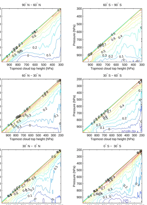
Figures 1 and 2 show, respectively, the vertical profile of cloud fraction P(z) and
172
∆P(z|ztop) in (7) derived from 1 month of data (July 2006) taken over 6 different
re-173
gions. ∆P(z|ztop) decreases monotonically with the distance from the uppermost cloud
174
top for a given uppermost cloud top height. When the distance is large, it sometimes
175
is negative in the southern hemisphere tropics. One possible reason for this is that the
CALIOP signal is sometimes completely attenuated while the CPR misses low-level clouds
177
so that low-level clouds occur less often than random overlap when mid and high level
178
clouds are present. Note that a large cloud fraction above the tropopause over the
Antarc-179
tic is in the original CALIPSO VMF data product and results for two reasons (D. Winker
180
personal communication 2009). First, it is sometimes difficult to identify the exact height
181
of tropopause over the Antarctica, and second, clouds that extend from the troposphere
182
into stratosphere are included in VFM data.
183
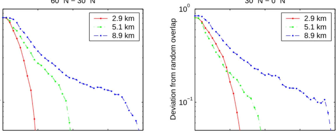
The assumption made in the previous section in deriving (12) is that ∆P in (7) decreases
184
exponentially with distance from the uppermost cloud top. Figure 3 shows ∆P as a
185
function of the distance from the uppermost cloud top for selected uppermost cloud top
186
heights. It indicates that ∆P decreases nearly exponentially with distance from the
187
uppermost cloud top for intermediate distance. A large correlation distance, hence a
188
smaller slope such as the 8.9 km case at the greater than 4 km from the uppermost cloud
189
top on the left side plot of Figure 3, might be an indication of precipitation. A small slope
190
near the cloud top might be caused by the finite thickness of clouds i.e. existence of a
191
minimum cloud thickness.
192
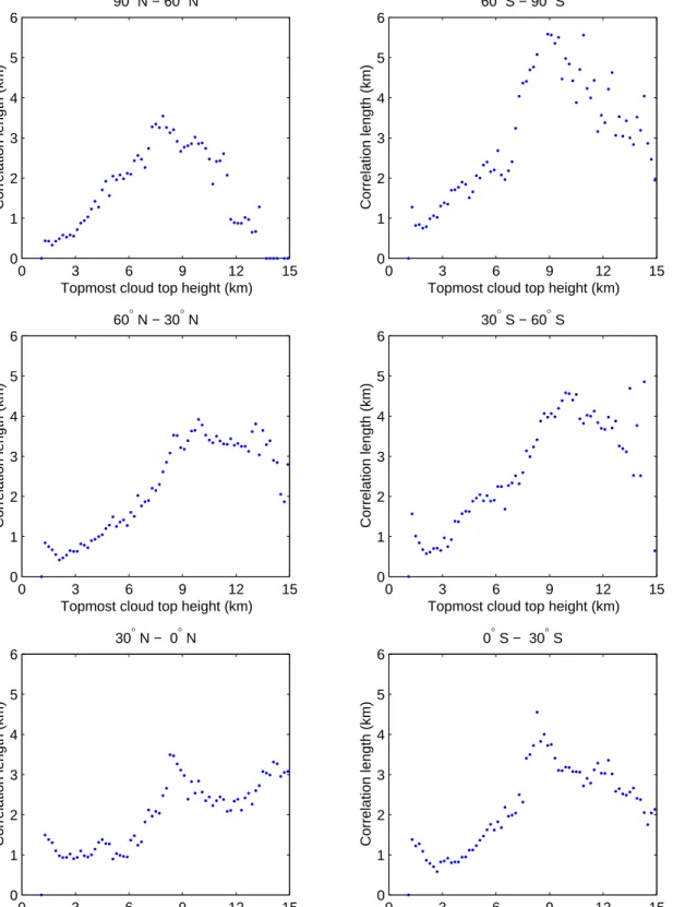
Because the inverse of the slopes of the lines shown in Figure 3 is the correlation
193
distance, the correlation distance as a function of the uppermost cloud top height can
194
be derived by a linear regression. However, Figure 3 indicates that the slope is not
195
constant throughout the atmospheric column for a given uppermost cloud top. Therefore,
196
applying a linear regression to the uppermost cloud top to the surface can leads to a biased
197
estimate. To reduce the error, we compute the slope using a 1.2-km moving window and
198
average all slopes so that a constant slope extending over the largest vertical length is
given the greatest weight. The result is plotted on Figure 4. As expected, the correlation
200
distance, which is the effective cloud thickness, increases with uppermost cloud top height.
201
When the uppermost cloud top height is larger than about 8 km, the correlation distance
202
becomes nearly constant and does not increase with height. This might be caused by
203
frequently occurring thin cirrus. The correlation length in the Tropics does not differ from
204
midlatitude values, probably because thick convective clouds does not occur frequently
205
even in the tropics compared with the occurrence of other cloud types [Dong et al. 2008].
206
The correlation distance derived here is related to the de-correlation length introduced
207
byHogan and Illingworth [2000] as indicated by (19) and (20). Those are not exactly the
208
same but the de-correlation distance, property which appears unique to GCMs, coincides
209
with the correlation distance of clouds defined in this paper when the cloud fraction of two
210
layers in the system are equal. Therefore, this result provides a physical interpretation of
211
the de-correlation distance, which might give some insight into how it is derived and how it
212
can be approximated when it is applied. Barker[2008a] speculates that the de-correlation
213
length depends on altitude. Because the above result indicates that the de-correlation
214
length is related to the effective cloud thickness and clearly the cloud thickness depends
215
on cloud type, we expect that the de-correlation length also depends on height.
216
The height dependence of the de-correlation distance is sometimes neglected when
pa-217
rameterizing the cloud overlap [Barker 2008a, Barker and P¨ais¨anen 2005]. The error in
218
the zonal and monthly mean TOA shortwave irradiance caused by neglecting the height
219
dependence of the de-correlation distance in computing the TOA shortwave irradiance is
220
less than 3 Wm−2 [Barker 2008a]. If the difference between the de-correlation distance
221
and the correlation distance gives a smaller TOA irradiance change compared with the
TOA irradiance change caused by neglecting height dependence of the de-correlation
dis-223
tance, the cloud correlation distance introduced here might be used as the de-correlation
224
distance for a cloud overlap parameterization.
225
To obtain a rough estimate of the sensitivity of the TOA reflected shortwave irradiance to the correlation distance, we use (12) and take a derivative with respect to D,
∂P(zk, ztop,k)
∂Dl
=−zl−zk
D2l P(zl, ztop,l)[1−P(zl)]e
−(zl−zk)/Dl, (21)
where the layer l is the upper layer. The actual cloud fraction in a layer depends on the
226
vertical depth of the layer, but Figure 1 suggests that P(zl, ztop,l) = P(zl) ≈ 0.25 can
227
be used as a rough estimate. If we further assume that Dl = 2 km, and zl −zk = 2
228
km, a 0.5 km error in Dl gives about a 0.1 cloud fraction error in P(zk, ztop,k). If we use
229
a typical value of ≈ −40Wm−2 for a zonal mean TOA shortwave cloud forcing in the
230
Tropics and 0.6 for a zonal mean cloud fraction exposed to space (e.g. Kato et al. [2008]),
231
a 0.1 cloud fraction change gives about 7 Wm−2 difference at TOA. Therefore, a rough
232
estimated tolerance of the correlation distance that gives an equivalent TOA shortwave
233
change by neglecting height dependence of de-correlation length is about 0.4 km. Figure
234
4 shows that the variability of the correlation distance among for uppermost cloud top
235
heights that are within ≈ 1 km of each other is on the order of 0.5 km. We expected
236
that the 0.1 cloud fraction change is the upper bound, hence this tolerance value would
237
be an underestimate for the following reason. UsingDl =zl−zk in the estimate gives the
238
largest cloud fraction change because a maximum of the function zl−zk
D2l e−(zl−zk)/Dl occurs 239
when zl−zk =Dl. In addition, the the correlation distance varies with height more than
240
that caused by the uppermost cloud top variation within≈1 km (Figure 4), which is also
241
an indication that neglecting height dependence has a larger effect on TOA irradiances.
Earlier studies indicate that the variability of TOA shortwave irradiance is mostly
243
caused by the variability of the cloud fraction exposed to space [Loeb et al. 2007]. The
244
relationship among the uppermost cloud top, correlation distance, and cloud fraction
sug-245
gests that the cloud fraction exposed to space changes by the correlation length and the
246
cloud fraction in the vertical layers. In the above two-layer system, the effective cloud
247
thickness Dl determines whether the fraction of clouds in the k layer vertically extends
248
from the l layer or the clouds exposed to space to become the uppermost cloud layer k.
249
The sensitivity of the cloud fraction expose to the space to the correlation distance is
250
largest when the k and l layers are separated by the distance Dl.
251
Earlier studies (e.g. Barker et al. [2003]) indicate that the cloud fraction exposed to
252
space largely depends on the assumed type of cloud overlap. Whether switching from the
253
random to the maximum cloud overlap assumption can lead to a significant improvement
254
in the TOA shortwave irradiance depends on the error in the correlation length and cloud
255
fraction in the vertical layers. If errors in the correlation length and the cloud fraction in
256
vertical layers are large, adopting a proper cloud overlap assumption may not significantly
257
improve TOA irradiance estimates. The change in the cloud fraction exposed to space due
258
to changing to the maximum/random cloud overlap assumption from the random cloud
259
overlap assumption in a two cloud layer system is ∆P(zk, ztop,l) = P(zl)[1−P(zl)]e −zl−zk
Dk .
260
This term is greater than the change in the cloud fraction exposed to space caused by the
261
error in the correlation length if zi−zj
D2i ∆Di is less than unity, which is possible as long as 262
the error in the correlation distance does not exceed 100% near the cloud base. Similar to
263
the above two-cloud layer example, if we useP(zl) = 0.25 andDl=zl−zk, the change in
the cloud fraction exposed to space due to changing the overlap assumption ∆P(zk, ztop,l)
265
is 0.19.
266
The sensitivity of the cloud fraction exposed to space due to the error in the cloud fraction is ∂P(zk, ztop,k) ∂P(zk) = 1− m X i=k+1 P(zi, ztop,i). (22)
The second term on the right side is the cloud fraction exposed to space above the kth
267
layer. Comparing (22) with ∆P(zk, ztop,l) = P(zl)[1−P(zl)]e−zlDk−zk, if the cloud fraction
268
error in thekth layer is smaller than the upper-layer cloud fraction in a two layer system,
269
the error in the cloud fraction exposed to space due to the error in the cloud fraction
270
is smaller than ∆P(z, ztop). Therefore, the improvement of the TOA irradiance estimate
271
caused by adopting a proper cloud overlap parameterization is large if the upper layer
272
cloud fraction is large.
273
5. Summaries and Conclusions
We combined vertical cloud profile from CALIPSO and CloudSat to utilize the strength
274
of each instrument and to understand vertical cloud profile quantitatively. We introduced
275
the cloud frequency of occurrence matrix that contains the vertical cloud profile as a
276
function of uppermost cloud top. When we assume that the cloud overlap approaches
277
the random overlap as the distance between the two cloud layers increases and define the
278
e-folding distance of the cloud occurrence probability deviating from the random overlap,
279
the uppermost cloud top and the cloud fraction vertical profiles can be related. The
280
e-folding distance, or correlation distance, is interpreted as the effective cloud thickness.
281
Cloud vertical profiles derived from CALIOP and CPR shows that the cloud occurrence in
layers below the uppermost cloud layer deviating from the random overlap nearly decays
283
exponentially. However, the data show that the correlation distance is not necessarily
284
constant throughout the atmospheric column for a given uppermost cloud top height. A
285
large correlation distance might be an indication of precipitation and the change of the
286
correlation distance might be used to screen precipitation.
287
In a two-cloud layer system, the correlation distance is equivalent to the de-correlation
288
distance introduced by Hogan and Illingworth [2003] when the upper and lower cloud
289
fractions are the same. Therefore, the de-correlation distance, which appears to be a
290
parameter somewhat unique to general circulation models, is linked to the effective cloud
291
thickness.
292
Appendix A: The effect of the vertical bin size
If we assume the conditional probability of cloud occurrence decreases exponentially with the distance from the uppermost cloud top
p(zj|ztop,i) =e−zji/Di, (a1)
where p(zj|ztop,i) is the probability of cloud occurrence in a thin layer and zji = zi−zj. The mean probability of cloud occurrence in the uppermost layer of ∆zi thickness is
P(zi|ztop,i) = 1 ∆zi Z ∆zi 0 e −z/Didz = Di(1−e−∆zi/Di) ∆zi . (a2)
When ∆zi/Di ¿1,P(zj|ztop,i)≈1. The mean probability of cloud occurrence in the jth layer of which thickness is ∆zj and zji distance from the uppermost cloud top layer i is
P(zj|ztop,i) = 1 ∆zj Z zji+∆zj/2 zji−∆zj/2 e −z/Didz = Die −zji Di µ e ∆zj 2Di −e −∆zj 2Di ¶ ∆zj . (a3)
The conditional probability then becomes P(zj|ztop,i) P(zi|ztop,i) = ∆ziezjiD µ e∆2Dzj −e −∆zj 2Di ¶ ∆zj µ 1−e−Di∆zi ¶ . (a4)
When ∆zj/D¿1, the conditional probability is
P(zj|ztop,i)
P(zi|ztop,i) ≈e
−zji/Di. (a5)
293
Appendix B: The relation between cloud fraction and uppermost cloud top profiles
The conditional probability of the cloud occurrence in the jth layer given the uppermost cloud top is in the ith layer is the sum of the probability due to a random overlap and a maximum overlap,
P(zj|ztop,i) =P(zj) + [1−P(zj)] exp [−(zi−zj)/Di]. (b1) Because P(zj|ztop,i)P(zi, ztop,i) = P(zj, ztop,i) andPmi=jP(zj, ztop,i) = P(zj), when we mul-tiply (b1) by P(zi, ztop,i) and sum up from i=j tom, then
P(zj) = m X i=j P(zi, ztop,i)P(zj) + m X i=j P(zi, ztop,i)[1−P(zi)] exp [−(zi−zj)/Di]. (b2) This expression leads to (14).
294
Appendix C: Cloud merging and grouping process
The CALIPSO and CloudSat cloud masks, obtained from the VFM and CLDCLASS
295
products, respectively are independent and sometimes can differ significantly due to
char-296
acteristics of the instrument used. This allows three combinations when the CALIPSO
and CloudSat masks are paired: 1) CALIPSO is cloud-free in the column and CloudSat
298
reports clouds, 2) CALIPSO reports clouds and CloudSat is cloud-free in the column, and
299
3) both CALIPSO and CloudSat report clouds somewhere in the column. If only one of
300
the paired profiles is valid, the valid profile is used without altering the profile.
301
After identifying the three cloud mask combinations described above, the cloud masks
302
are compared at each vertical layers from each instrument. The vertical resolution of
303
CALIPSO profile is 30 m below the altitude of 8 km and 60 m above the altitude of 8
304
km [Winker et al. 2007]. The vertical resolution of CloudSat profile is 240 m throughout
305
[Stephens et al. 2008]. Comparing the cloud masks layer by layer, identical profiles
306
are grouped. Where both the CALIPSO and CloudSat profiles are cloudy, all CALIPSO
307
profiles match and all CloudSat profiles match for it to be grouped together. If the number
308
of resulting groups is less than 16, all groups are kept. If that number is exceeded, similar,
309
less populous profiles are combined together until the number becomes less than or equal
310
to 16.
311
The process to reduce the number of cloud groups when it exceeds 16 is as follows. First, the number of unique profiles within a case, CALIPSO cloudy CloudSat cloud-free profiles, CALIPSO cloud-cloud-free CloudSat cloudy profiles, and CALIPSO and CloudSat cloudy profiles, is determined by
nfj = 16 Ni j P3 i=1Nii 16 P3 i=1nii , (c1)
where N is the number of profiles in the case, n is the number of unique profiles in the
312
case (i.e. N > n) and superscript i and f, respectively, indicate the initial and final. If
313
the number of unique profiles in the case is within the limit, no combining is done for
314
the case. If the limit is exceeded, all unique profiles that contain nine or more matches
are kept. Then starting with the remaining profile with the most exact matches, other
316
profiles that only differ by one are combined with it. If this fails to reduce the number
317
of profiles below the limit, the last step is repeated combining profiles that differ by an
318
increasing number of layers until the limit is met.
319
The number of cloud profiles in a CERES footprint is sometimes nearly 50 (Figure 5).
320
This cloud grouping process reduces the number of profiles to less than or equal to 16.
321
The area covered by different cloud profiles grouped together is less than 10% for most
322
of CERES footprints. As a result, the cloud profiles are not altered very much from the
323
original CALIOP and CPR cloud profiles (Figure 6). The number of vertical layers in
324
a profile before the algorithm reduces it to the maximum of 6 is less than 6 for most of
325
merged profiles (Figure 7). 99.68
326
Acknowledgments. We thank Drs. David Winker, Charles Trepte, Mark Vaughan,
327
Gerald Mace, Roger Marchand, and Robert Holz for helpful discussions. The work was
328
supported by the NASA Science Mission Directorate through the NASA Energy Water
329
Cycle Study (NEWS) project.
330
References
Barker, H. W. (2008a), Representing cloud overlap with an effective de-correlation length:
331
An assessment using CloudSat and CALIPSO data J. Geophys. Res., 113, D24205,
332
dio:10.1029/2008JD010391.
333
Barker, H. W, (2008b), Overlap of fractional cloud for radiation calculation in GCMs: A
334
global analysis using CloudSat and CALIPSO data, J. Geophys. Res., 113, D00A01,
335
dio:10.1029/2007JD009677.
Barker, H. W. and P. P¨aos¨anen, (2005), Radiative sensitivities for cloud structural
proper-337
ties that are unresolved by conventional GCMsJ. Q. R. Meteorol. Soc., 131, 3103-3122.
338
Barker, H. W., and co-authors, (2003), Assessing 1D atmospheric solar radiative transfer
339
models: interpretation and handling of unresolved clouds, J. Climate, 16, 2676-2699.
340
Chang, F.-L., and Z. Li, (2005), A new method for detection of cirrus-overlapping-water
341
clouds and determination of their optical properties. J. Atmos. Sci., 62, 3993-4009.
342
Dong, X., B. A. Wielicki, B. Xi, Y. Hu, G. G. Mace, S. Benson, F. Rose, S. Kato, T.
343
Charlock, and P. Minnis, (2008), Using observations of deep convective systems to
344
constrain atmospheric column absorption of solar radiation in the optically thick limit,
345
J. Geophys. Res., 113, D10206, doi:10.1029/2007JD009769.
346
Hogan, R. J., and A. J. Illingworth, (2003), Parameterizing ice cloud inhomogeneity and
347
he overlap of inhomogeneities using cloud radar data, J. Atmos. Sci.,, 60, 756-767.
348
Hogan, R. J., and A. J. Illingworth, (2000), Deriving cloud overlap statistics from radar,
349
Q. J. R. Meteorol. Soc., 126, 2903-2909.
350
Jacob, C., and S. A. Klein, (2000), A parameterization of the effect of cloud and
pre-351
cipitation overlap for use in general-circulation models, Q. J. R. Meteorol. Soc., 126,
352
2525-2544.
353
Kato, S, F. G. Rose, D. A. Rutan, and T. P. Charlock, (2008), Cloud effects on the
354
meridional atmospheric energy budget estimated from Cloud and the Earth’s Radiant
355
Energy System (CERES) data, J. Climate, 21, 4223-4241.
356
Loeb, N. G. B. A. Wielicki, F. G. Rose, and D. R. Doelling (2007), Variability in global
357
top-of-atmosphere radiation between 2000 and 2005, Geophys Res. Lett, 34, L03704,
358
doi:10.1029/2006GL028196.
Mace, G. G., and S. Benson-Troth, (2002), Cloud-layer overlap characteristics derived
360
from long-term cloud radar data, J. Climate, 15, 2505-2515.
361
Minnis, P., J. Huang, B. Lin, Y. Yi, R. F. Arduini, T.-F. Fan, J. K. Ayers, and G. G.
362
Mace (2007), Ice cloud properties in ice-over-water cloud systems using TRMM VIRS
363
and TMI data, J. Geophys. Res., 112, D06206, doi:10.1029/2006JD007626.
364
Smith, G. L. (1994), Effects of time response on the point spread function of a scanning
365
radiometer, Appl Opt., 30, 7031-7037.
366
Stephens, G. L. and co-authors, (2002), The CloudSat mission and a-train, Bull. Amer. 367
Meteor. Soc., 83, 1771-1790.
368
Stephens, G. L., and co-authors, (2008), CloudSat mission: performance and
369
early science after the first year of operation, J. Geophys. Res., 113, D00A18,
370
doi:10.1029/2008JD009982.
371
Wang, L., and A. E. Dessler, (2006), Instantaneous cloud overlap statistics in the
372
tropical area revealed by ICESat/GLAS data, Geophys. Res. Lett., 33, L15804,
373
doi:10.1029/205GL024350.
374
Will´en, Ulrika, S. Crewell, H. K. Baltink, and O. Sievers, (2005), Assessing model
pre-375
dicted vertical cloud structure and cloud overlap with radar and lidar ceilometer
obser-376
vations for the Baltex Bridge Campaign, Atmos. Res., 75, 227-255.
377
Winker, D. M., W. H. Hunt, and M. J. Mcgill, (2007), Initial performance assessment of
378
CALIOP, Geophys. Res. Lett., 34, L19803, doi:10.1029/2007GL030135.
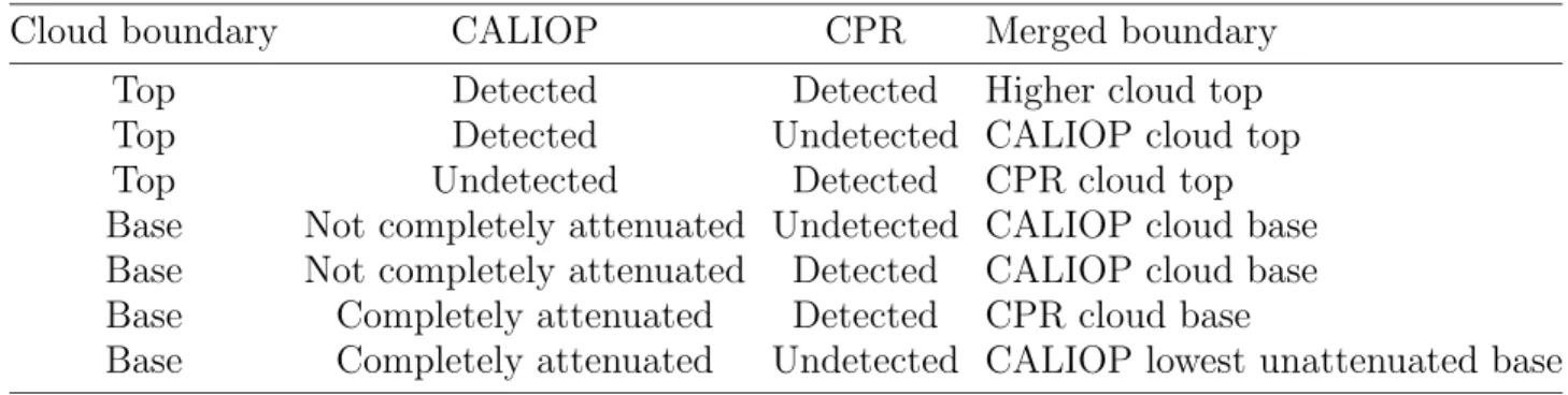
Table 1. Cloud mask merging strategy
Cloud boundary CALIOP CPR Merged boundary Top Detected Detected Higher cloud top Top Detected Undetected CALIOP cloud top Top Undetected Detected CPR cloud top Base Not completely attenuated Undetected CALIOP cloud base Base Not completely attenuated Detected CALIOP cloud base Base Completely attenuated Detected CPR cloud base
Base Completely attenuated Undetected CALIOP lowest unattenuated base
0.0 0.1 0.2 0.3 0.4 0.5 0.6 1000 900 800 700 600 500 400 300 200 100 Frequency of occurrence Pressure (hPa) 90° N−60° N 60° N−30° N 30° N−0° N 0.0 0.1 0.2 0.3 0.4 0.5 0.6 1000 900 800 700 600 500 400 300 200 100 Frequency of occurrence Pressure (hPa) 30° S−0° S 30° S−60° S 60° S−90° S
Figure 1. Cloud faction vertical profile derived from CALIPO and CPR merged cloud profiles computed with 200 m resolution for July 2006. left) northern hemisphere and right) southern hemisphere.
900 800 700 600 500 400 300 900 800 700 600 500 400 300
Topmost cloud top height (hPa)
Pressure (hPa) 90° N − 60° N 0 0.1 0.10.2 0.2 0.3 0.3 0.4 0.4 0.5 0.5 0.6 0.6 0.7 0.7 0.8 900 800 700 600 500 400 300 200 900 800 700 600 500 400 300 200
Topmost cloud top height (hPa)
Pressure (hPa) 60° N − 30° N 0 0.1 0.1 0. 0.1 0.2 0.2 0.3 0.3 0.4 0 0.4 0.4 0.5 0.5 0.6 0.6 0.7 0 0.7 0.8 0.8 0.9 900 800 700 600 500 400 300 200 900 800 700 600 500 400 300 200
Topmost cloud top height (hPa)
Pressure (hPa) 30° N − 0° N 0 0 0 0.1 0.1 0.10.2 0.30.2 0.3 0.3 0.4 0.4 0.5 0.5 0.5 0.6 0.6 0.7 0.7 0.8 0.8 900 800 700 600 500 400 300 200 900 800 700 600 500 400 300 200
Topmost cloud top height (hPa)
Pressure (hPa) 0° S − 30° S 0 0 0.1 0.1 0.1 0.2 0.2 0.3 0 0.3 0.4 0 0.4 0.4 0.5 0.5 0.6 0 0.6 0.7 0.7 0 8 0.8 0.9 0.9 900 800 700 600 500 400 300 200 900 800 700 600 500 400 300 200
Topmost cloud top height (hPa)
Pressure (hPa) 30° S − 60° S −0. 0 0 0.1 0. 1 0.1 0.2 0.2 0.2 0.3 0.3 0.3 0.4 0 4 0.4 0.5 0.5 0.6 0.6 0.7 0.8 0.9 900 800 700 600 500 400 300 900 800 700 600 500 400 300
Topmost cloud top height (hPa)
Pressure (hPa) 60° S − 90° S 0 0 0.1 0.1 0.2 02 0.2 0.3 0 0.3 0.4 0.4 0.5 0.5 0.6 0.60.7
Figure 2. Deviation from the random overlap ∆P defined in (9) as a function of uppermost cloud top height for 6 different regions. Cloud vertical profiles derived from July 2006 CALIOP and CPR data are used.
0 2 4 6 8 10−1
100
60° N − 30° N
Distance from the cloud top (km)
Deviation from random overlap
2.9 km 5.1 km 8.9 km 0 2 4 6 8 10−1 100 30° N − 0° N
Distance from the cloud top (km)
Deviation from random overlap
2.9 km 5.1 km 8.9 km
Figure 3. Deviation from the random overlap ∆P as a function of distance from the uppermost cloud top for three uppermost cloud top heights.
0 3 6 9 12 15 0 1 2 3 4 5 6
Topmost cloud top height (km)
Correlation length (km) 90° N − 60° N 0 3 6 9 12 15 0 1 2 3 4 5 6
Topmost cloud top height (km)
Correlation length (km) 60° N − 30° N 0 3 6 9 12 15 0 1 2 3 4 5 6
Topmost cloud top height (km)
Correlation length (km) 30° N − 0° N 0 3 6 9 12 15 0 1 2 3 4 5 6
Topmost cloud top height (km)
Correlation length (km) 0° S − 30° S 0 3 6 9 12 15 0 1 2 3 4 5 6
Topmost cloud top height (km)
Correlation length (km) 30° S − 60° S 0 3 6 9 12 15 0 1 2 3 4 5 6
Topmost cloud top height (km)
Correlation length (km)
60° S − 90° S
Figure 4. Correlation length derived from one month (July 2006) of CALIOP and CPR of data as a function of uppermost cloud top height for 6 different regions.
0 10 20 30 40 50 0 0.2 0.4 0.6 0.8 1
Number of cloud groups
Cumulative occurrence 0 5 10 15 20 25 30 0 0.02 0.04 0.06 0.08 0.1 Cloud cover (%) Frequency of Occurrence
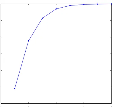
Figure 5. Left) Cumulative distribution of the number of cloud groups in a CERES footprint. The blue line indicates the actual number of profile cumulative distribution and the red line indicates the cumulative distribution after reducing to the maximum of 16 groups in a footprint. Right) Cloud fraction of cloud groups greater than or equal to the 11th cloud group number. The cloud group number having the largest cloud fraction over a footprint is 1 and the largest cloud number is assigned to the cloud group having he smallest cloud fraction.
−90 −60 −30 0 30 60 90 0.55 0.6 0.65 0.7 0.75 0.8 0.85 0.9 0.95 1 Latitude Cloud fraction −90 −60 −30 0 30 60 90 −5 0 5x 10 −3 Latitude
Cloud fraction difference
−2 0 2 4 6 x 10⁻³ 1000 900 800 700 600 500 400 300 200 100
Cloud fraction difference
Pressure (hPa) −4 −2 0 2 4 x 10⁻⁴ 1000 900 800 700 600 500 400 300 200 100
Cloud top fraction difference
Pressure (hPa)
a) b)
c) d)
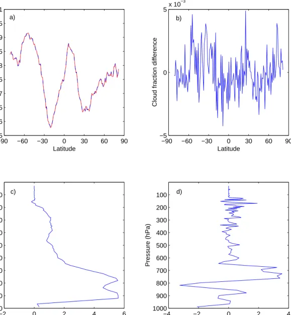
Figure 6. a) Cloud fraction exposed to space as a function of latitude derived from CALIPSO-CloudSat merged cloud profile before grouping (solid line) and after grouping (dash-dot line). The difference (after grouping minus before grouping) of the zonal mean cloud fraction exposed to space b), the difference in the cloud fraction vertical profile c), and uppermost cloud top fraction vertical profile d).
0
2
4
6
8
0.4
0.5
0.6
0.7
0.8
0.9
1
Number of layers
Cumulative occurrence
Figure 7. Cumulative occurrence of the number of vertical cloud layers in a CALIPSO-CloudSat merged cloud profile.