Analytical Evaluation of Cellular Network Uplink
Communications with Higher Order Sectorization
Deployments
Jianhua He, Wenyang Guan, Weisi Guo, Wei Liu, and Wenqing Cheng
Abstract—Higher Order Sectorization (HOS), which splits macro base stations into a larger number of sectors, is widely considered in the cellular community as a cost-effective means of improving network capacity. We develop two general and low-complexity analytical models to characterize and relate the uplink performance indicators with key dynamic functionalities and variables, such as fractional power control (FPC), directional antenna radiation patterns and the multi-cell inter-cell interfer-ence (ICI). The adopted methodology approximates the uplink ICIs from individual cell sectors by log-normal random variables, of which the statistical parameters can be estimated using approaches that trade-off complexity and accuracy. Furthermore, the aggregate uplink ICI is approximated with a log-normal random variable, from which network performance metrics are computed. Compared to two existing baseline analytical methods the proposed analytical models have improved accuracy. The analytical models are applied to evaluate HOS deployments with both regular and irregular cell geometries. Results on sectorization scaling show it is an effective method in capacity scaling, but at the cost of increased outage probability. The proposed theoretical models can be used as a fast and effective tool for performance assessment and optimization of Long-Term Evolution (LTE) and 5G networks.
Index terms— LTE; Cellular networks; 5G; Higher order sectorization; Uplink communications; Performance modelling
I. INTRODUCTION
T
HE increasing proliferation of affordable smart phones, and the fusion of social-media and multi-media content delivery is driving a strong growth in wireless network traffic. While the baseline Long-Term Evolution (LTE) standards represent a significant capacity improvement, new capacity scaling methods are needed to meet the demands of the future 5G standard [1]–[3]. As a result, emerging system architectures and radio techniques such as small cells, massive and multi-user multiple input multiple output (MIMO), 3D-beamforming, millimeter wave transmission, non-orthogonal multiple access (NOMA) and software defined networks (SDN) have been investigated extensively [1]–[6].Jianhua He (email: [email protected]) is with the School of
En-gineering and Applied Science, Aston University, UK. Wenyang Guan
(email: [email protected]) is with School of Computer
and Information Engineering, Beijing Technology and Business
Uni-versity, China. Weisi Guo (email: [email protected]) is
with School of Engineering, University of Warwick, UK. Wei Liu
(email:[email protected], Corresponding Author) and
Wen-qing Cheng (email: [email protected]) are with the School of
Electronic Information and Communications, Huazhong University of Science and Technology, China.
One of the most cost-effective means of improving network capacity has been, and remains to be higher order sector-ization (HOS). HOS is cost-efficient by exploiting spatial spectrum reuse without incurring significant capital or op-erational expenditures, and remains attractive compared to deploying new eNodeBs or frequency carriers [10]–[14]. HOS has been widely evaluated in the cellular community both analytically, numerically, and experimentally [7]–[14]. In the baseline configuration of LTE networks, macrocell eNodeBs are equipped with 3 sectors. Although HOS with 6, 12 or even more sectors per macrocell BS has the potentials of enhancing network capacity, its implementation remains rare. Complementary technologies include adopting MIMO techniques with 12 antennas per site [10]. But compared to the capacity achieving multi-user MIMO technology with 3 antennas per sector, HOS with single antenna transmission per sector produced higher mean site throughput [11]. Throughput and fairness performance of HOS with and without cooperative transmission schemes were analyzed with up to 12 antennas per site [12]. HOS and fractional frequency reuse (FFR) schemes were jointly evaluated by simulation and analysis for orthogonal frequency division multiple access (OFDMA) downlink communication [14]. However, HOS also comes with its own challenges in terms of inter-cell interference (ICI), power control, and mobility management. A fast and effective analytical tool is in high demand for feasibility assessment and optimization of large-scale HOS deployment.
Whilst a great deal of research attention has been given to LTE and 5G networks downlink performance, low complexity computational methods for uplink performance evaluation and optimization remains lacking, especially for HOS. Perfor-mance evaluation of cellular wireless networks was more focused on downlink modelling (e.g., [14], [16]–[20]), and somewhat neglected in uplink research [21]–[23]. The com-plexity of the uplink modelling is greater, as the interference arises from mobile users (as opposed to fixed base stations on the downlink) and more advanced power control schemes are used for uplink communication which further complicates the modelling process [20].
In the literature the existing research studies on modelling cellular network uplink ICI and network performance can be classified into three major categories.
a) Deterministic geometry models: The majority of stud-ies on cellular network uplink communication modeling fall into this category. A widely used model for the uplink ICI is Wyner model [25], in which ICI was assumed to be a
weight of aggregate signals transmitted from adjacent cells and the ICI value is left to be determined. It was shown in [26] that the Wyner model is not accurate for cellular networks employing time-division multiple access (TDMA) or OFDMA technologies. Haas and McLaughlin provided a derivation of probability distribution function (PDF) of adjacent channel interference from single cell in the uplink of a cellular system [27]. Similarly Zhu et al. derived PDF of single cell uplink ICI with power control in OFDMA networks [28]. It is noted that aggregate ICI expression is not derived from the PDF of single cell uplink ICI [27] [28], and uplink signal to interference and noise ratio (SINR) and network throughput are not analyzed. Elayoubi et al.studied the uplink ICI and capacity in LTE systems without shadowing [29]. Karray studied uplink resource allocation and network performance in both code-division multiple access (CDMA) and OFDMA networks [30]. A framework of modeling uplink ICI was reported with scheduling in [31] and with power com-pensation schemes in [32]. Generalized K-composite fading was assumed for analytical model tractability. The model is complex and considers one tier of regularly laid interfering cells. Singh et al. developed a moment-matched log-normal modeling of uplink ICI with power control and shadowing for CDMA system [33]. The aggregate uplink ICI is assumed to be log-normally distributed. The moment-matched approach was applied to OFDMA networks with sector antennas for networks without shadow fading [34]. A simplified version of the approach was used to analyze uplink performance with partial frequency reuse scheme [35]. It is noted that large network performance prediction errors are observed from the model with shadowing.
b) Stochastic geometry models: Stochastic geometry has been widely applied for cellular network performance analysis [36]–[38]. A fluid model assuming uniformly distributed BSs was used to analyze uplink ICI and uplink power com-pensation, but the model was not verified [39]. Norlan et al. applied the stochastic geometric tool to model OFDMA uplink ICI and network performance [22]. The model was extended by ElSawy et al. for cellular uplink transmission with truncated power control [36], [40]. Tabassum et al. modelled uplink NOMA in large-scale cellular networks using Poisson cluster processes [38]. It is noted that the stochastic geometric model for uplink transmission is not thoroughly verified by simulations and a limitation with the model is that it is not directly applicable to practical cellular network with irregular cellular shapes, or with sector antennas which may cause an interfering user to be closer to the site location than the target user.
c) Hybrid model and contributions: Tabassum et al. applied their analytical framework to analyze uplink ICI and capacity in two-tier small cell networks [41]. In the analysis macrocell BSs are assumed to have fixed locations and small cell BSs are assumed to be randomly located. The analytical model is complex and considers the generalized K-composite fading.
One common weakness of the current uplink models is that the above models are complex and do not take into account sectorized antenna patterns except [34], and practical link level
performance models are not used in these models. Shadow fad-ing, which is an inherent nature of wireless communications, is not considered in [34]. We extend our preliminary work in [23] to develop an unified and simple analytical models for LTE network uplink communications, and apply the analytical models to investigate LTE network performance with HOS deployments.
II. SYSTEMMODEL
A. Network Layout and Resource Allocation
In this paper, we consider LTE networks with antenna configurations of 1, 3, 6 and 12 sectors per site. For the 3-sectors configuration, a clover-leaf network layout is used1. Using these network layouts, let us consider a cellular network withNsites sites. The eNodeBs are labeled from 1 toNsites. Without loss of generality eNodeB 1 is set as the target eNodeB, located at the origin (0, 0). The inter-site distance is denoted byRISD.
The number of sectors per site is denoted byNa, set to 1, 3, 6 and 12 in this paper. So the total number of sectors (denoted by Nsect) equals NsitesNa. The jth sector of the nth site is denoted by As,j, where s ∈ [1, Nsites] and j ∈ [1, Na]. For
ease of notation, sector As,j and its sector antenna (SA) are
also labeled by n, with n = (s−1)Na+j, s ∈ [1, Nsites],
j∈[1, Na], andn∈[1, Nsect]. Letϑs,jdenotes the horizontal
angle of the main radiation direction of sector As,j, which is
set to(j−1)∗π/Na−ϑs,1for (j∈[2, Na]), withϑs,1=−π/6 for the 3-sectors and−π/12 for the 6-sectors and 12-sectors settings, respectively.
In LTE networks single carrier frequency division multiple access (FDMA) is chosen for uplink multiple access. SC-FDMA has most of the merits of OSC-FDMA but has a lower peak to average power ratio (PAPR). With SC-FDMA spectrum resources are split up into a number of parallel orthogonal narrow-band sub-carriers with a space of 15 kHz, which are then organized into resource blocks for allocation. An LTE uplink radio frame consists of 20 slots of 0.5 ms each, and one subframe consists of two slots. Each slot carries either 6 or 7 SC-FDMA symbols for short and long cyclic prefix (CP) configurations, respectively. The resource grid for the uplink comprises a number of resource blocks in the frequency-time domains. The minimum resource for allocation has a granularity of 1 ms in time domain and a granularity of 180 kHz (i.e., 12 subcarriers) in frequency domain. The eNodeB allocates unique time-frequency resources to users, which eliminates intra-cell interference but not inter-cell interference. For ease of notation, we define a physical resource block (PRB) as the minimum resource used for transmission with 180 kHz by one symbol.
We assume a round-robin scheduler for resource allocation. A universal frequency reuse scheme is used, which means the available network frequency resource is used by every sector of the eNodeBs. We assume a fully loaded network, in which all the available resource blocks are allocated to the users in the
1For the 3-sectors BS case, the clover-leaf network layout was found to
sectors. Users are assumed to be uniformly distributed within the network.
Table I lists the main notations used in this paper.
B. Channel Model and Antenna Radiation Pattern
Since we consider a fully loaded network, without loss of generality, we can focus our study on one sector (say sector 1) by investigating the performance of users located in sector 1 with one PRB.
Let us consider a general userukserved by sectork, where
k∈[1, Nsect].
Define the signal powerPn,uk received by sectornfrom a user uk , which is expressed by:
Pn,uk=P t
ukGPL(n, uk)GA(n, uk)ψn,uk, (1)
where Putk is the transmit power from user uk over a PRB, GPL(n, uk)is the path loss between the site of sector nand
useruk,GA(n, uk)is the antenna gain between sectornand
useruk, andψn,uk is the shadow fading between sectornand useruk. For ease of notation, we letPn,ur k denote the received power by sector nfrom useruk without shadowing:
Pn,ur
k =P t
ukGPL(n, uk)GA(n, uk). (2)
The antenna gain GA(n, uk) models the gain of the antenna
in the direction between sector nand useruk:
GA(n, uk) =GA,maxGA,h,v(ϑn,uk, θn,uk), (3)
whereGA,maxis the maximum antenna gain, andGA,h,v(ϑ, θ) is the 3-dimensional antenna radiation pattern with horizontal angle ϑ and vertical angle θ between a considered pair of sector and user.
The shadow fadingψn,uk models the variability of the path loss between sectornand useruk, which is assumed to follow
a log-normal distribution. According to [43], the Gaussian random variables that characterize the log-normal shadowing are assumed to have a zero mean and a standard deviation of σw. For simplicity, the shadowing between users and the sectors is assumed to be uncorrelated.
C. Fractional Power Control
Uplink power control has a great impact on achieving a required SINR, while at the same time controlling the interference caused to neighboring cells. In a classic power control scheme, all users are expected to receive the same SINR in uplink. An alternative power control scheme, FPC, which was approved by 3GPP, is used in the paper. With the FPC scheme users with a higher path loss can operate at a lower SINR and thus generate less inter-cell interference [21]. Suppose that the path loss and the antenna gain between a general user un and its serving sector is GPL(n, un) and GA(n, un), respectively. According to the FPC and the
afore-mentioned notations, we can use the following formula to determine the transmit power from the userun:
Putn=minPmax, PtargetM h
GPL(n, un)GA(n, un)
i−β
, (4)
whereβ is the power compensation factor [21], taking values of 0, 0.4 to 1 with a step of 0.1;M is the number of PRBs allocated to a user, which is set to 1 in this paper. Pmax is the maximal uplink transmit power on a PRB, andPtarget is a configurable target received power.
III. SINR EXPRESSION ANDEXISTINGANALYTICAL
MODELS
A. General Expression of SINR
As assumed in Section II, we focus our analysis on the performance of users associated with sector1, based on which the overall network performance can be calculated.
Taking into account the previous definitions, the SINR (denoted by γu1) for a general target user u1 within sector 1 can be calculated as:
γu1 = P1,u1 Nsect P n=2 P1,un+δ 2 = P r 1,u1ψ1,u1 Nsect P n=2 Pr 1,unψ1,un+δ 2 , (5)
whereδ2 is the noise power.
As shadow fadingψ1,un is assumed to be independent for all users un within sector n, we can useψn to represent the
shadow fading between any interfering userun from sectorn
and sector 1, and rewrite the expression in (5) for SINR:
γu1 = Pr 1,u1ψ1,u1 Nsect P n=2 Pr 1,unψn+δ 2 . (6)
LetIn denote the uplink ICI generated from sectorn(2≤ n ≤ Nsect) without shadowing, and its mean and variance denoted byInandIbn respectively. The mean and variance of Inwill be calculated in Section IV. LetIw,ndenote the uplink
ICI generated from sector n (2 ≤n≤Nc) with shadowing.
We haveIw,n=Inψn. Let Isum denote the sum of the single sector interference Iw,n (2 ≤ n ≤ Nsect), which is Isum = PNsect
n=2Iw,n. Let Isum andIbsum denote the mean and variance of Isum.
With the above definitions for the uplink ICI, the expression in (6) for SINR can be further rewritten as:
γu1 = Pr 1,u1ψ1,u1 Nsect P n=2 Inψn+δ2 = P r 1,u1ψ1,u1 Isum+δ2 . (7)
B. Existing Analytical Models
The main challenge of modeling uplink interference and network performance comes from the dynamic positions of the interfering users. Although the moments of single cell interference In has been computed and used in the literature
(such as mean and variance), there is no simple and well-established model proposed to approximate the distribution of In, which hinders the development of effective analytical
models for uplink communications of LTE and other OFDMA based cellular networks. In this subsection we briefly discuss two existing analytical approaches used for uplink communi-cations of cellular networks.
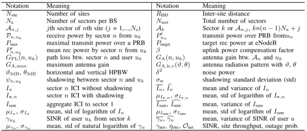
TABLE I NOTATIONS
Notation Meaning Notation Meaning
Nsite Number of sites RISD Inter-site distance
Na Number of sectors per BS Nsect Total number of sectors
An,j jth sector ofnth site (j = 1,...,Na) Ak SectorkorAn,j,k=(n−1)Na+j
Pn,uk receive power by sectornfromuk P
t
un transmit power over PRB fromun
Pmax maximal transmit power over a PRB Ptarget target rec power at eNodeB
Pn,ur k mean rec power by sectornfromuk β uplink power compensation factor
GPL(n, uk) path loss btw. sectorn and useruk GA(n, uk) antenna gain btw.An anduk
GA,max maximum antenna gain GA,h,v(ϑ, θ) antenna radiation pattern withϑ,θ
ϑ3dB,θ3dB horizontal and vertical HPBW δ2 noise power
ψn,uk shadowing between sectornanduk σw shadowing standard deviation (std)
In sectornICI without shadowing In,Ibn mean and variance ofIn
Iw,n sectornICI with shadowing µIw,n,σIw,n mean, std of logarithm ofIw,n
Isum aggregate ICI to sector 1 Isum,Idsum mean, variance ofIsum
µIn, σIn mean, std of logarithm ofIn µIsum,σIsum mean, std of logarithm ofIsum
γuk SINR of useruk from sectork γu, cγu mean, variance of SINR of useru
µγu,σγu mean, std of natural logarithm ofγu γnet,ηsite,Onet SINR, site throughput, outage prob.
1) Moment Matching Analytical Model: An analytical ap-proach was originally proposed to model the uplink ICI for cel-lular networks with assumption of multiple intra-cell and inter-cell interferers [33]. Shadow fading, power control and inter-cell association were taken into account in the analytical model. The approach was applied in [34] to evaluate interference and network throughput of OFDMA cellular networks with fractional frequency reuse but without considering shadowing and power control.
The main idea used in this approach is that the aggregate ICI
Isumis approximated as a log-normal random variable, without any assumption on the distribution of the single cell ICIs. According to the log-normal assumption for Isum, Isum can be uniquely characterised by its mean and variance (Isum and
b
Isum). To determine the mean and variance ofIsum, a moment matching method was proposed in [33] to match the mean and variance of Isum to the values which are related to the mean and variance of single sector ICIs.
Once the mean and variance (IsumandIbsum) of the aggregate ICI Isum are computed, we can compute the mean network-wide spectrum efficiency and throughput with the method presented in Section IV. The analytical model based on the idea of moment matching for the aggregate ICI in [33] [34] is called moment matching model (MoM model) in this paper.
2) Sum of Means Analytical Model: In this model shadow-ing is not considered [35]. The mean of sshadow-ingle sector ICI is simply summed up to approximate the aggregate ICI Isum. Then the SINR for a given user u1 without shadowing is computed by the following formula:
γu1 = P1r,u1 Nsect P i=2 Ii+δ2 ≈ P r 1,u1 Nsect P i=2 In+δ2 . (8)
From (8), mean network-wide spectrum efficiency and throughput can be computed. This simple analytical model with the approach of summing up the mean single sector ICI as the aggregate ICI is called sum of means (SoM) model.
IV. PROPOSEDANALYTICALMODELS
A. Uplink ICI Observation and General Framework
Through network simulations it is observed that the MoM and SoM analytical models can be used for system perfor-mance evaluation of cellular networks without shadowing, but the models show poor performance when shadowing is taken into account.
In [23] the single cell ICIs with shadowing was as-sumed to follow log-normal distribution in the case of omni-directional antennas, which enables simple analytical modeling of OFDMA based cellular networks. Next we investigate how well the single sector ICIs and aggregate ICI with shadowing can be approximated by log-normal random variables.
Multi-cell simulations were run to obtain the values of the single sector and the aggregate ICI with shadowing (8 dBσw), for the four antenna settings: 1, 3, 6 or 12 sector antennas per site Na, with RISD=500 m, and power compensation factor
β = 0.4. The number of samples Nsp for each setting onNa is 20000. Representative results on the log-normal fit to the single sector ICIs (from sectors 3, 6, 9 and 12) for the 3 sectors per site setting are presented in Fig. 1. Log-normal fittings to the aggregate ICI for the four Na settings are presented in Fig. 2. It can be observed from the histogram plots that the fittings for the single sector and aggregate ICIs by log-normal distributions are good.
Furthermore, we measure the goodness of fit quantitatively on the simulated single sector ICIs by log-normal distribution with the Anderson-Darling (AD) test [44]. The key of the AD test is the computation of the AD statistic value (denoted by
ADn for the nth sector ICI test) with the following formula
[44]: ADn=−Nsp− Nsp X i=1 2i−1 Nsp n ln[F(Yn,i)]+ln[1−F(Yn,Nsp−i+1)] o (9) where Nsp denotes the number of samples used in an AD test, Yn,i denotes the ith data of the ordered simulated ICI
samples from sectorn, ln(x)is the natural logarithm function,
F(x) denotes the cumulative distribution function for the log-normal distribution. The distribution parameters for the hypothesized log-normal distribution are estimated from the simulation sector ICI samples. For a given critical value, if the computed AD statistic value ADn is smaller than a
specific critical value, then the hypothesis H1 that the sector
n ICI comes from the hypothesized log-normal distribution can be accepted. The critical value for AD test is dependent on the significance level [44], for example the widely used significance levels of 1% and 5% gives critical values of 1.035 and 0.752, respectively.
The above AD test procedure is applied to all the interfering sectors as well as the sector of interest (i.e. Sector 1) separately for the four Na settings. The AD statistic values for the received power by Sector 1 and all the interfering sector ICIs are presented in Fig. 3(d). Comparing the AD statistic values of the sectors to the critical value 1.035, we can confirm that a large majority of sector ICIs follow log-normal distribution, and the remaining sectors have ICIs closely following log-normal distribution. For example, for the case of Na=1, the AD value for 14 out of the 18 interfering sectors is less than the critical value, and the other 4 sectors also have an AD value of less than 1.6. For the case of Na=3, the AD value for 51 out of 56 sectors is smaller than 1.035, which means 51 sector ICIs follow log-normal distribution according to the AD test.
According to the experiment results, we can make the following assumption with high confidence: the single sector ICIs with shadowing (Iw,n for n∈[2, Nsect]) are independent log-normal random variables.
Single sector interference with shadowing×10-14
0 0.5 1 1.5 2 2.5 3 3.5 4 Frequency of occurance 0 500 1000 1500 2000 2500 3000 3500 4000 Simulation samples Fitting distribution (a) Sector 3.
Single sector interference with shadowing×10-14
0 0.2 0.4 0.6 0.8 1 Frequency of occurance 0 500 1000 1500 2000 2500 3000 3500 Simulation samples Fitting distribution (b) Sector 6.
Single sector interference with shadowing×10-14
0 0.5 1 1.5 2 Frequency of occurance 0 500 1000 1500 2000 2500 3000 3500 4000 Simulation samples Fitting distribution (c) Sector 9.
Single sector interference with shadowing×10-14
0 0.2 0.4 0.6 0.8 1 Frequency of occurance 0 500 1000 1500 2000 2500 3000 3500 4000 Simulation samples Fitting distribution (d) Sector 12.
Fig. 1. Density of single sector ICIs with 8 dB shadowing with the 3 sectors per site setting, from a) sector 3; b) sector 6; c) sector 9 and d) sector 12.
β=0.4.
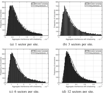
With the assumption of the single sector ICIs being log-normal random variables, the aggregate ICI can be approx-imated by a log-normal random variable with widely used
Aggregate interference with shadowing ×10-12 0 0.5 1 1.5 2 2.5 3 Frequency of occurance 0 100 200 300 400 500 600 Simulation samples Fitting distribution
(a) 1 sector per site.
Aggregate interference with shadowing ×10-12
0 0.5 1 1.5 2 Frequency of occurance 0 100 200 300 400 500 600 700 800 Simulation samples Fitting distribution
(b) 3 sectors per site.
Aggregate interference with shadowing ×10-13
0 1 2 3 4 5 6 7 Frequency of occurance 0 100 200 300 400 500 600 700 Simulation samples Fitting distribution
(c) 6 sectors per site.
Aggregate interference with shadowing ×10-12 0 0.2 0.4 0.6 0.8 1 Frequency of occurance 0 100 200 300 400 500 600 Simulation samples Fitting distribution
(d) 12 sectors per site.
Fig. 2. Log-normal fitting of aggregate ICI with 8 dB shadowing, under
different settings on the number of sectors per siteNaof : a) 1; b) 3; c) 6;
and d) 12.β= 0.4.
Sector ID
0 5 10 15 20
Anderson-Darling test statistic value
0 0.2 0.4 0.6 0.8 1 1.2 1.4 1.6
(a) 1 sector per site.
Sector ID
0 10 20 30 40 50 60
Anderson-Darling test statistic value
0 2 4 6 8 10 12 14
(b) 3 sectors per site.
Sector ID
0 20 40 60 80 100 120
Anderson-Darling test statistic value
0 2 4 6 8 10 12 14 16 18
(c) 6 sectors per site.
Sector ID
0 50 100 150 200 250
Anderson-Darling test statistic value
0 5 10 15 20 25 30 35
(d) 12 sectors per site. Fig. 3. AD test statistic value of sector ICIs with 8 dB shadowing, under
different settings on the number of sectors per siteNaof : a) 1; b) 3; c) 6;
and d) 12.β= 0.4.
analytical tools for addition of multiple log-normal random variables.
Next we propose two analytical approaches to compute the single sector ICI Iw,n for a general sector n, based on
which two analytical models are developed correspondingly to compute system level performance metrics of interest. The two proposed analytical models are called log-normal mean (LoM) model and log-normal log-normal (LoL) model, respectively. With both LoM and LoL models the aggregate ICI is approximated by a log-normal random variable. But the single sector ICIs without shadowing are modelled by their means in the LoM model and by log-normal random variables
in the LoL model, respectively. More details on the LoM and LoL models are presented later.
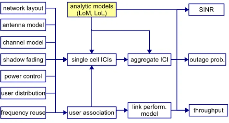
The overall analytical framework based on the proposed analytical models is shown in Fig. 4. It is general and can take into account various cellular deployment geometries, antenna radiation patterns, channels models, user distributions, and link performance models. According to the received signal strength from the sectors in the network, users are first associated to the sector with the strongest received signal. Then we can compute the single sector ICIs and the aggregate ICI. The aggregate ICI model combined with given link performance models can be used to compute network performance metrics of interest.
Fig. 4. General analytical framework.
a) LoM Model: In the analytical model LoM, Iw,n (for n∈[2, Nsect]) is approximated by the product of the mean of
In and the shadowingψn:
Iw,n ≈ Inψn. (10)
As the mean of single sector ICI without fading is a determin-istic variable and the shadowing is a log-normal variable, it is easy to compute the mean and variance of the single sector ICI
Iw,nwith shadowing as a log-normal random variable. Then the
aggregate ICI as a sum of the log-normal approximated ICI from multiple sectors is also approximated as a log-normal random variable.
b) LoL Model: The LoM model is simple and has much higher accuracy than the MoM and SoM models, but the prediction error is still large when shadowing is present. In the second analytical model, the single sector ICIs without shading are also approximated by log-normal random variables.
B. Approaches to Compute Single Sector ICI Iw,n
For a general log-normal variable x, it can be uniquely characterised by the meanµand standard deviationσfor the variablex’s natural logarithm. The probability density function
fLN(x;µ, σ)of the log-normal variablexcan be expressed by:
fLN(x;µ, σ) =
1
xσ√2πe
−(lnx−µ)2
2σ2 . (11)
Let µw,n and σw,n denote the mean and standard
devia-tion of the normal logarithm of Iw,n. Next we present the
approaches to determine the key parameters µw,n and σw,n
for the log-normal distribution associated with the single sector ICI Iw,n, used in the LoM and LoL models, respectively.
1) Computation of Mean and Variance ofIn: Letρndenote
the user density in sectorn,n∈[1, Nsect]. With the assumption of uniform user locations, we have ρn = area of sector1 n. At a
given time, consider a general user un served by sector n.
With given locations for userun, sector 1 (target sector) and
sector n, we can compute the distance D1,un between user
un and sector 1 and the distanceDn,un between userun and sector n. Then the interference contributed from user un of
sectorncan be computed withPr
1,un from (2).
Without loss of generality, suppose userun is located with
polar coordinates (rn,θn) relative to its serving sector (sector n). The mean and variance of single sector ICI In can be
computed by integrating the interference contributed from user
un over sectorn, for n= 2, ..., Nsect:
In= Z Z An P1r,u nρnrndrndθn, (12) b In = Z Z An P1r,un−In 2 ρnrndrndθn, (13) wherePr
1,unis a function ofuncoordinates (rn,θn). The inte-grals (12) and (13) can be calculated by traditional numerical quadrature tools.
2) LoM Model: With the approximation used for LoM model, we can computeµw,n andσw,n forIw,n for analytical
model LoM using the following approach:
µw,n = log(In), (14)
σ2w,n = σw2. (15)
3) LoL Model: With LoL model, single sector ICIs without shadowing are also assumed to be log-normal variables. Letµn
andσ2
ndenote the mean and variance of the natural logarithm
of In, for n ∈ [2, Nsect], respectively. µn and σ2n can be
calculated fromIn andIbn by:
σn2 = ln1 + Ibn In , (16) µn = ln(In)− σ2n 2 . (17)
As single sector ICI with shadowing is approximated by the product of two log-normal random variable in LoL model, we can compute µw,n andσw,n for Iw,n for LoL model:
µw,n = µn, (18)
σw2,n = σ2n+σ2w. (19)
Now we can see the main difference between LoM model and LoL model: for LoM model, formulas (14) and (15) are used to compute µw,n and σw,n of Iw,n; whereas for LoL
model formulas (18) and (19) are used.
C. Aggregate InterferenceIsum
The aggregate interference Isum is the sum of the single sector ICIs from the interfering sectors (independent log-normally distributed random variables). There is no closed-form expression for the distribution of Isum, but it can be reasonably approximated by another log-normal distribution
(e.g., with commonly used Fenton method [45] or Schwartz-Yeh method [46]).
Let µsum andσsum denote the mean and standard deviation of the normal logarithm of Isum, respectively, which can be computed according to Fenton method [45].
Then from µsum andσsum, the mean (denoted byIsum) and variance (denoted by Ibsum) of the aggregate ICI Isum can be obtained by: Isum = eµsum+σ 2 sum/2, (20) b Isum = (eσ 2 sum−1)Isum. (21)
D. SINR and Network Throughput
Statistically users located in the target sector (sector 1) experience the aggregate ICI following the same log-normal distribution. Without loss of generality, let us consider a general useruin the target sector. The SINRγu for useruis
calculated as:
γu =
P1,u
Isum+δ2
. (22)
LetVIN=Isum+δ2. For model tractability,δ2is treated as a log-normal variable with mean oflog(δ2)and standard devi-ation of 0 for its logarithm. Then we can approximateVIN by a new log-normal variable, with mean and standard deviation denoted byµINandσINfor its logarithm, respectively.µINand
σIN can be calculated by Fenton approximation method again [45].
Now asP1,uandVINare modelled as two independent log-normal variables, the SINR γu of user ucan be modelled as
a log-normal variable. Let µγu andσγu denote the mean and standard deviation of the normal distribution associated with
γu, which can be computed according to the properties of
log-normal random variables by the following formulas:
µγu = ln(P r 1,u)−µIN, (23) σγ2u = σ 2 w+σ2IN. (24)
Let γu and bγu denote the mean and variance of SINR of
user u, respectively, which can be computed using formulas similar to (20) and (21): γu = eγu+γ 2 u/2, (25) b γu = (eγ 2 u−1)γ u. (26)
Let (r, θ) denote the polar coordinates of a general user u
from sector 1. The network-wide mean SINR (denoted byγnet) can be obtained by integration of single user SINR γu over
sector1:
γnet=
Z Z
A1,1
γuρ1rdrdθ. (27)
It is noted thatγuis a function of coordinates (r, θ) of useru.
For a user with an instantaneous SINRγu, we suppose that
there is a link layer performance modelF(.)that can map a SINRγuto spectral efficiency (bps/Hz). LetCuandCudenote
the instantaneous and average spectrum efficiency (bps/Hz) of useru, respectively, which are calculated by:
Cu = F(γu), (28)
Cu =
Z ∞
0
F(x)fLN(x;µγu, σγu)dx. (29)
LetCnetdenote the average spectrum efficiency (bps/Hz) of sectorA1 which is calculated by:
Cnet= Z Z
A1,1
Cuρ1rdrdθ. (30)
The mean site throughput (denoted by ηsite) in bps can be computed with network bandwidthBnetby:
ηsite=NaCnetBnet. (31)
Suppose that a user is out of service if its instantaneous SINR is lower than a given outage thresholdγout. LetOu and
Onetdenote the outage probability of the general useru, which can be calculated by:
Ou = Z γout 0 fLN(x;µγu, σγu)dx, (32) Onet = Z Z A1,1 Ouρ1rdrdθ. (33) V. NUMERICRESULTS A. System Configurations
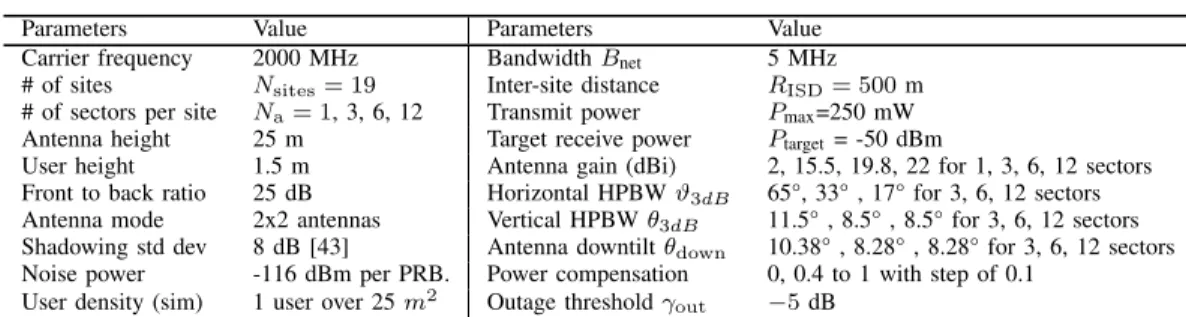
Analytical results are obtained with Matlab numerical tools, while simulation results are obtained by system level simulator and averaged over 105 simulations runs. The simulator is written in Matlab by the authors following the simulation framework of the Vienna LTE simulator developed for down-link communications [16]. Table II presents the most relevant system parameters. In the simulations, users are uniformly distributed in the networks and are associated to the sector with the strongest received signal among all the sectors. The same given channel model, antenna radiation pattern, power control strategies, and LTE link level performance model are used for both simulation and modelling. It is noted that the proposed analytical models are general and can be used with other system configurations.
The path loss model specified in [43] for outdoor line-of-sight communications is used,
GPL(d) =−34.02−22log10(d) [dB]. (34) wheredis the distance between a consider pair of an eNodeB site and a user.
We use the radiation patternGA,h,v(ϑ, θ)provided in [43]:
GdBA,h,v(ϑ, θ) = −min(−(GdBA,h(ϑ) +GdBA,v(θ)), GdBFront),
GA,h,v(ϑ, θ) = 10G
dB
A,h,v(ϑ,θ)/10. (35) whereGA,h(ϑi,j,u) andGA,v(θi,j,u) are the normalized
hor-izontal and vertical radiation pattern offset of the considered sector antenna, andGdB
TABLE II SYSTEM SETTINGS
Parameters Value Parameters Value
Carrier frequency 2000 MHz BandwidthBnet 5 MHz
# of sites Nsites= 19 Inter-site distance RISD= 500m
# of sectors per site Na= 1, 3, 6, 12 Transmit power Pmax=250 mW
Antenna height 25 m Target receive power Ptarget= -50 dBm
User height 1.5 m Antenna gain (dBi) 2, 15.5, 19.8, 22 for 1, 3, 6, 12 sectors
Front to back ratio 25 dB Horizontal HPBWϑ3dB 65°, 33° , 17° for 3, 6, 12 sectors
Antenna mode 2x2 antennas Vertical HPBWθ3dB 11.5° , 8.5° , 8.5° for 3, 6, 12 sectors
Shadowing std dev 8 dB [43] Antenna downtiltθdown 10.38° , 8.28° , 8.28° for 3, 6, 12 sectors
Noise power -116 dBm per PRB. Power compensation 0, 0.4 to 1 with step of 0.1
User density (sim) 1 user over 25m2 Outage thresholdγout −5dB
GA,h(ϑi,j,u)andGA,v(θi,j,u)are approximated as [43]:
GdBA,h(ϑ) = −min(12|ϑ| ϑ3dB ,25), (36) and GdBA,v(θ) =−min(12|θ−θdown| θ3dB ,20), (37)
where ϑ3dB and θ3dB are the horizontal and vertical half-power beamwidth (HPBW), and θdown is the down-tilt angle. The values for the antenna parameters are shown in Table II. For the numerical evaluation, we use a spectral efficiency function F(x), which approximates an abstracted LTE link level model developed from the LTE link level Simulator [16], with 2x2 antenna mode, open loop spatial multiplexing (OLSM) and adaptive modulation and coding (AMC). The original LTE link model (presented in Fig.9 of [16]) mapping channel SNR (dB) to spectral efficiency (bps/Hz) is approxi-mated by a polynomial function presented in [14].
B. Network Performance with Regular Cellular Layout
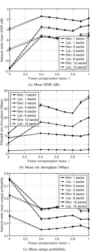
Fig. 5(a), Fig. 5(b) and Fig. 5(c) present the network per-formance (obtained by simulations and the proposed analytical model LoL), in terms of mean network SINR (dB), mean site throughput (Mbps) and mean outage probability, against the uplink power compensation factor β, for RISD = 500m and
σw= 8 dB, respectively. The number of sectors per eNodeB is set to 1, 3, 6 and 12 in the experiments.
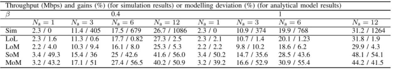
Table III provides more details about the mean site through-put for different system configurations. In Table III, the row with labels ‘Sim’ shows the site throughput obtained by simulations with various numbers of sectors per site and the relative throughput gains with respect to the omni-directional antenna setting; the rows starting with model names show the site throughput obtained by different analytical models and the absolute modeling deviation in percents with respect to the simulation results.
From Fig. 5, it can be observed that analytical results with model LoL match very well to the system-level simulation results, with less than 1.5% average difference. The overall average difference between the analytical model LoL and system-level simulation results is 1.46% for the scenario of
σw=8 dB. This fact shows the accuracy of the proposed analytical model, one of the main contribution of this paper. In addition, the analytical models are significantly faster than simulations. Simulations took more than 60 hours to produce
the whole simulation results presented in this paper, while analytical models only took 10 minutes. The accuracy and high computation efficiency enable the use of the proposed analytical tools as an effective method to predict network performance in a fast and reliable manner. For example, opti-mization tools that attempt to find proper antenna orientation and down-tilt in HOS deployments can use the proposed analytical models to quickly search over different candidate configurations and find the best performing one.
a) Impact of Power Compensation and Sector Antennas:
The power compensation factor β is set to 0 and from 0.4 to 1 with a step of 0.1. The impact of power compensation is obvious. The network performance (SINR, throughput and outage probability) is at the worst without power compensation (β=0), and is close to the best with full power compensation (β=1).
If we compare the settings with different number of sectors per site, it can be observed from Fig. 5 that:
• The average network SINR decreases with number of sec-tors per site except for the case of omni-directional antenna setting due to the larger ICI introduced by the extra sectors per site.
• The average site throughput increases with number of sectors per site due to the lager spatial reuse.
• The outage probability changes similarly as the network SINR with increasing number of sectors per site. It is noted that the setting of 3 sectors per site gives the lowest outage probability of around 0.35, which is still large and strongly indicates the use of advanced interference mitigation schemes.
It is interesting to note that doubling the number of sectors per site from 3 to 6 almost doubles the site throughput with β=1. Increasing the number of sectors per site from 6 to 12 leads to an around 50% increase of throughput (see Table III for detailed analysis of average site throughput gains). This indicates that HOS can be used as an effective way of increasing network capacity, but the throughput gains diminish with the increasing number of sectors due to stronger inter-cell interference.
b) Comparison of Analytical Models: Next we compare the proposed analytical models (LoL and LoM) to two existing models (SoM and MoM). Numerical results against power compensation factor β are presented in Fig. 6 with σw = 8 dB. It is noted that the moment-matching approach is used in [33] to compute the uplink ICI only and is used in [35] to
TABLE III
MEAN SITE THROUGHPUT AND GAIN OVER OMNI-DIRECTIONAL ANTENNA SETTING
Throughput (Mbps) and gains (%) (for simulation results) or modelling deviation (%) (for analytical model results)
β 0.4 1 Na= 1 Na= 3 Na= 6 Na= 12 Na= 1 Na= 3 Na= 6 Na= 12 Sim 2.3 / 0 11.4 / 405 17.5 / 679 26.7 / 1086 2.3 / 0 10.9 / 374 19.9 / 768 31.2 / 1264 LoL 2.3 / 1.6 11.3 / 0.6 17.7 / 0.82 27.3 / 2.5 2.3 / 2.1 10.7 / 1.4 20.1 / 1.23 31.8 / 1.9 LoM 2.2 / 4.0 10.3 / 9.4 16.1 / 8.0 25.3 / 5.3 2.2 / 2.2 9.8 / 10.2 18.6 / 6.2 29.9 / 4.3 SoM 3.4 / 49.3 15.4 / 36 25 / 42.6 41.6 / 56.0 3.4 / 50.2 14.7 / 35.6 28.5 / 43.6 48.1 / 54.1 MoM 3.2 / 43.2 17.1 / 51 27.4 / 56.5 40.2 / 50.9 3.2 / 39.2 16.6 / 52.9 30.9 / 55.4 44.2 / 41.5
compute network capacity without shadowing. The approach is extended in this paper to produce SINR and site throughput results with shadowing.
It can be observed that model LoL significantly outperforms the other models for all the investigated cases. The overall modelling deviation to the simulation results for models LoL, LoM, SoM and MoM is 1.46%, 16.9%, 43.6%, 66.8%, respec-tively. The accuracy of LoM model is the closest to that of LoL model. In most cases, model LoM underestimates the network throughput but the prediction is reasonably good, except at two occasions of Na = 6 and Na = 12 with
β = 0, where throughput obtained with LoM model is much higher than the simulation one. If these two occasions are excluded, considering thatβ= 0is not widely used for uplink communications, the average modelling deviation of model LoM to simulation results is 8.2%, which can be acceptable for fast performance evaluation with reduced computation complexity.
C. Network Performance with Irregular Cellular Layout
A controlled irregular cellular layout is created by introduc-ing a random movement of(rand−0.5)×125meters in both x-axis and y-axis directions to all the hexagonally laid out eNodeB sites except the target eNodeB site, whererandis a uniform random variable in [0,1]. Representative results for the average site throughput are presented in Fig. 7(a) withNa= 3. Again model LoL produces good performance prediction for all the investigated system configurations. Model LoM gives the second best performance, while models SoM and MoM largely overestimate the network throughput. Similar trends on the site throughput with increasing number of sectors can be observed for the irregular cellular layout.
VI. CONCLUSION
In this paper we have developed a unified analytical frame-work to characterize and relate the uplink performance indica-tors with key dynamic functionalities and variables. We have proposed two analytical approaches to compute the uplink ICIs from single sectors, which are approximated as log-normal random variables. The analytical approaches have a tradeoff on computation complexity and modeling accuracy. Based on the analytical approaches two analytical models (model LoM and model LoL) have been developed to compute the network performance of interest. Compared to the two existing analytical methods which use moment matching approach for aggregated ICI and the means of single sector ICIs, the proposed analytical models have better model accuracy,
which are verified by system level simulations. The average difference between the results obtained by simulations and our model LoL is less than 1.5% under the investigated system setting with inter-site distance of 500 m. The analytical models were applied to LTE network with HOS deployments with both regular and irregular cellular layouts. It has been observed that increasing the number of sectors per site can effectively improve the uplink throughput. Moving from 3-sectors to sectors doubles the site throughput and moving from 6-sectors to 12-6-sectors gives another 50% increase. However, the capacity improvement is achieved at the cost of increased outage probability due to the high spatial reuse with HOS.
ACKNOWLEDGMENT
This project has received funding from the European Unions Horizon 2020 research and innovation programme under the Marie Skodowska-Curie grant agreement No 824019 and the FP7 grant DETERMINE under the FP7-PEOPLE-2012-IRSES grant agreement No 318906.
REFERENCES
[1] M. Shafiet al., “5G: A Tutorial Overview of Standards, Trials,
Chal-lenges, Deployment, and Practice,” IEEE Journal on Selected Areas in
Communications, Vol. 35, No. 6, pp. 1201 - 1221, June 2017. [2] S. Parkvall, E. Dahlman, A. Furuskar, M. Frenne, “NR: The New 5G
Radio Access Technology,”IEEE Communications Standards Magazine,
Vol. 1, No. 4, pp. 24-30, Dec. 2017.
[3] T.Tran, A. Hajisami, P. Pandey, D. Pompili, “Collaborative Mobile Edge Computing in 5G Networks: New Paradigms, Scenarios, and
Challenges,”IEEE Communications Magazine, Vol. 55, No. 4, pp. 54
-61, April 2017.
[4] M. Al-Kadri et al., “Full-Duplex Small Cells for Next Generation
Heterogeneous Cellular Networks: A Case Study of Outage and Rate
Coverage Analysis,” IEEE Access, Vol. 5, pp. 8025-8038, May 2017.
[5] A. Heet al., “Spectral and Energy Efficiency of Uplink D2D Underlaid
Massive MIMO Cellular Networks,” IEEE Transactions on
Communi-cations, Vol. 65, No. 9, Sept. 2017.
[6] H. Elkotby, M. Vu, “Interference Modeling for Cellular Networks
Under Beamforming Transmission,” IEEE Transactions on Wireless
Communications, Vol. 16, No. 8, pp. 5201-5217, Sept. 2017.
[7] B. Hagermanet al., “WCDMA 6-sector deployment- case study of a
real installed UMTS-FDD network,”in Proc. of IEEE VTC’06, 2006.
[8] A. Osseiran and A. Logothetis, “Smart antennas in a WCDMA radio
network system: modeling and evaluations,” IEEE Transactions on
Antennas and Propagation, Vol. 54, No. 11, pp. 3302-3316, Nov. 2006. [9] A. Osseiran, P. Skillermark and M. Olsson, “Multi-antenna SDMA in
OFDM radio networks systems: modeling and evaluations,”in Proc. of
IEEE PIMRC’07, 2007.
[10] H. Huanget al., “Increasing downlink cellular throughput with limited
network MIMO coordination,” IEEE Transactions on Wireless
Commu-nications, Vol. 8, No. 6, pp. 2983-2989, June 2009.
[11] H. Huanget al., “Increasing throughput in cellular networks with
higher-order sectorization,” in Proc. Asilomar’10, 2010.
[12] I. Riedel and G. Fettweis, “Increasing throughput and fairness in the
downlink of cellular systems with N-fold sectorization,” in Proc. of
Power compensation factor β
0 0.2 0.4 0.6 0.8 1
Network wide mean SINR (dB)
-12 -10 -8 -6 -4 -2 0 Sim: 1 sector LoL: 1 sector Sim: 3 sector LoL: 3 sector Sim: 6 sector LoL: 6 sector Sim: 12 sector LoL: 12 sector
(a) Mean SINR (dB).
Power compensation factor β
0 0.2 0.4 0.6 0.8 1
ENodeB site throughput (Mbps)
0 5 10 15 20 25 30 35 Sim: 1 sector LoL: 1 sector Sim: 3 sector LoL: 3 sector Sim: 6 sector LoL: 6 sector Sim: 12 sector LoL: 12 sector
(b) Mean site throughput (Mbps).
Power compensation factor β
0 0.2 0.4 0.6 0.8 1
Network wide mean outage probability
0.3 0.4 0.5 0.6 0.7 0.8 Sim: 1 sector LoL: 1 sector Sim: 3 sector LoL: 3 sector Sim: 6 sector LoL: 6 sector Sim: 12 sector LoL: 12 sector
(c) Mean outage probability.
Fig. 5. Network-wide performance with different number of sector antennas.
RISD= 500m, power compensation factorβ= 1,σw= 8 dB.
[13] R. Joyce and L. Zhang, “Higher order horizontal sectorisation gains for
a real 3GPP/HSPA+ network,”in Proc. European Wireless, 2013.
[14] J. He et al., “Analytical evaluation of higher order sectorization,
fre-quency reuse and user classification methods in OFDMA networks,”
IEEE Transactions on Wireless Communications, Vol. 15, No. 12, pp. 8209-8222, Dec. 2016.
[15] J. Ermanet al., “Over The Top Video: The Gorilla in Cellular Networks,”
ACM SIGCOMM, 2011.
[16] Mehlfuhrer et al., “The Vienna LTE simulators - Enabling reproducibility
in wireless communications research,” EURASIP Journal on Advances
in Signal Processing, pp.1-14, 2011:29, 2011.
[17] L. Chenet al., “System-level simulation methodology and platform for
Power compensation factor β
0 0.2 0.4 0.6 0.8 1
ENodeB site throughput (Mbps)
0 5 10 15 20 25 30 35 Simulation Model LoL Model LoM Model SoM Model MoM (a) Na= 6.
Power compensation factor β
0 0.2 0.4 0.6 0.8 1
ENodeB site throughput (Mbps)
0 10 20 30 40 50 Simulation Model LoL Model LoM Model SoM Model MoM (b)Na= 12.
Fig. 6. Mean site throughput (Mbps) of various analytical models against
power compensation factorβwithσw= 8 dB, for a)Na= 1; b)Na= 3; c)
Na= 6; d)Na= 12.
Power compensation factor β
0 0.2 0.4 0.6 0.8 1
ENodeB site throughput (Mbps)
6 8 10 12 14 16 18 Simulation Model LoL Model LoM Model SoM Model MoM
(a) Comparison of the analytical models withNa= 3.
Fig. 7. Mean site throughput (Mbps) against power compensation factorβ
with irregular cellular layout.σw= 8 dB.
mobile cellular systems,” IEEE Communications Magazine, Vol. 49,
No. 7, 2011.
[18] T. Bonald and A. Proutiere, “Wireless downlink data channels: user
performance and cell dimensioning,” In Proc. Mobicom’03, 2003.
[19] J. Andrews, F. Baccelli, and R. Ganti, “A tractable approach to coverage
and rate in cellular networks,” IEEE Transactions on Communications,
Vol. 59, No. 11, pp. 3122-3134, Nov. 2011.
[20] T. Novlan, R. Ganti, A. Ghosh, J. Andrews, “Analytical evaluation
of fractional frequency reuse for OFDMA cellular networks,” IEEE
Transactions on Wireless Communications, Vol. 10, No. 12, pp. 4294-4305, Dec. 2011.
[21] C. Castellanoset al., “Performance of uplink fractional power control
in UTRAN LTE,”In Proc. of IEEE VTC’08, 2008.
[22] T. Norlanet al., “Analytical modeling of uplink cellular networks,”IEEE
Transactions on Wireless Communications, pp.2669-2679, June 2013.
[23] J. Heet al., “Statistical model of OFDMA cellular networks uplink
inter-ference using Lognormal distribution,”IEEE Wireless Communications
Letters, Vol.2, No.5, pp. 575-578, Oct. 2013.
[24] B. Yang, W. Guo, Y. Jin and S. Wang, “Smartphone Data Usage:
Downlink and Uplink Asymmetry”, IET Electronics Letters, Vol. 52,
No. 3, 2015.
[25] A. Wyner, “Shannon-theoretic approach to a Gaussian cellular
multiac-cess channel,”IEEE Transactions on Information Theory, Vol. 40, No.
6, pp.1713-1727, Nov. 1994.
[26] J. Xu, J. Zhang, and J. Andrews, “On the accuracy of the Wyner model
in downlink cellular networks,”In Proc. IEEE ICC’11, 2011.
[27] H. Haas and S. McLaughlin, “A derivation of the PDF of adjacent
channel interference in a cellular system,” IEEE Communications
Letters, Vol. 8, No. 2, Feb. 2004.
[28] Y. Zhuet al., “Distribution of uplink inter-cell interference in OFDMA
networks with power control,” In Proc. IEEE ICC’14, 2014.
[29] S. Elayoubi and O. Haddada, “Uplink intercell interference and capacity
in 3G LTE systems,”In Proc. IEEE ICON’07, 2007.
[30] M. Karray, “Evaluation of the blocking probability and the throughput
in the uplink of wireless cellular networks,”In Proc. IEEE ComNet’10,
2010.
[31] H. Tabassumet al., “A framework for uplink intercell interference
mod-eling with channel-based scheduling,” IEEE Transactions on Wireless
Communications, Vol. 12, No. 1, pp. 206-219, Jan. 2013.
[32] H. Tabassumet al., “A statistical model of uplink inter-cell interference
with slow and fast power control mechanisms,” IEEE Transactions on
Communications, Vol. 61, No. 9, pp. 3953-3966, Sep. 2013.
[33] S. Singhet al., “Moment-matched lognormal modeling of uplink
inter-ference with power control and cell selection,” IEEE Transactions on
Wireless Communications, Vol. 9, No. 3, pp. 932-938, Mar. 2010. [34] H. Chang and I. Rubin, “Optimal downlink and uplink fractional
frequency reuse in cellular wireless networks,” IEEE Transactions on
Vehucular Technology, April 2015.
[35] L. Wang et al., “An analytical framework for multi-layer partial
fre-quency reuse scheme design in mobile communication systems,”IEEE
Transactions on Vehucular Technology, Nov. 2015.
[36] H. ElSawyet al., “Modeling and Analysis of Cellular Networks Using
Stochastic Geometry: A Tutorial,” IEEE Communications Surveys and
Tutorials, Vol. 19, No. 1, pp. 167-203, 1st Quater 2017.
[37] M. Haenggi, “User Point Processes in Cellular Networks,” IEEE
Wireless Communications Letters, Vol. 6, No. 2, pp. 258-261, April 2017.
[38] H. Tabassum, E. Hossain, and M. Hossain, “Modeling and Analysis of Uplink Non-Orthogonal Multiple Access in Large-Scale Cellular
Networks Using Poisson Cluster Processes,” IEEE Tranactions on
Communications, Vol. 65, No. 8, pp. 3555-3570, Aug. 2017. [39] M. Coupechoux and J. Kelif, “How to set the fractional power control
compensation factor in LTE?” in Proc. of IEEE Sarnoff Symposium,
May 2011.
[40] H. ElSawy and E. Hossain, “On stochastic geometry modeling of cellular uplink transmission with truncated channel inversion power control,”
IEEE Transactions on Wireless Communications, Vol. 13, No. 8, pp. 4454-4469, Aug. 2014.
[41] H. Tabassum et al., “Interference statistics and capacity analysis for
uplink transmission in two-tier small cell networks: a geometric
proba-bility approach,”IEEE Transactions on Wireless Communications, Vol.
13, No. 7, pp. 3837-3852, July 2014.
[42] M. Sheikh, and J. Lempiinen, “A flower tessellation for simulation
purpose of cellular network with 12-sector sites,” IEEE Wireless
Communications Letters, Vol. 2, No. 3, pp. 279-282, June 2013. [43] 3GPP TR 36.814 V9.0.0, “Further advancements for E-UTRA physical
layer aspects, Technical Report, March 2010.
[44] N. Razali, Y. Wah, “Power comparisons of Shapiro-Wilk,
Kolmogorov-Smirnov, Lilliefors and Anderson-Darling tests” Journal of Statistical
Modeling and Analytics, Vol. 2, No. 1, pp. 2133, 2011.
[45] L. Fenton, “The sum of log-normal probability distributions in scatter
transmission systems,” IEEE Transactions on Communications, Vol. 8,
No. 1, pp. 57-67, Mar. 1960.
[46] S. Schwartz and Y. Yeh, “On the distribution function and moments
of power sums with lognormal components, Bell System Technology
Journal, Vol. 61, No. 7, pp. 1441-1462, Sept. 1982.
Jianhua Hereceived his BSc and MSc degrees from Huazhong University of Science and Technology (HUST), China, and a PhD degree from Nanyang Technological University, Singapore, respectively. Dr He is a Lecturer at Aston University, UK. His main research interests include mobile communica-tions, 5G networks, connected vehicles, autonomous driving, Internet of things, AI for OCR and wireless newtorks. He has authored or co-authored over 100 technical papers in major international journals and conferences. He is an IEEE Senior Member.
Wenyang Guanreceived the B.Eng. degree in elec-tronic information engineering from Jilin University, China, in 2005, and the M.S. and Ph.D degree in advanced telecommunication from Swansea Univer-sity, Swansea, UK, in 2008 and 2013, respectively. From 2013 to 2015, he was a Postdoctoral Research Associate with Peking University. He is currently a lecturer in Beijing Technology and Business Univer-sity. His research interests include MIMO systems, FPGA programming and wireless communications.
Dr. Weisi Guo (S07-M11-SM16) is an associate professor at the University of Warwick and a Turing Fellow at the Alan Turing Institute. His expertise is in signal processing and networks, and has been PI on over 2.4m of funding in a variety of communica-tion and cyberphysical projects. He has published over 100 IEEE papers, won the IET Innovation Award, and been shortlisted for the Bell Labs Prize three times.
Wei Liu (M’06) received the B.S. degree in Telecommunication Engineering in 1999 and Ph.D. in Electronics and Information Engineering in 2004, both from Huazhong University of Science and Technology, Wuhan 430074, China. He is currently a professor with the School of Electronic Information and Communications, Huazhong University of Sci-ence and Technology. His research interests include network measurement, learning evalution, and etc.
Wenqing Cheng received the B.S. degree in Telecommunication Engineering in 1985 and Ph.D. in Electronics and Information Engineering in 2005, both from Huazhong University of Science and Technology, Wuhan 430074, China. She is currently a professor with the School of Electronic Infor-mation and Communications, Huazhong University of Science and Technology. Her research interests include communication systems, e-Learning appli-cations, and etc.