ASPECTS CONCERNING A DYNAMIC
MODEL FOR A SYSTEM WITH TWO
DEGREES OF FREEDOM
M. BOTI
Ş
1C. HARBIC
1Abstract: In this article is presented a dynamic model for a system with two degrees of freedom and the controller used for control in position. The dynamic model uses Lagrangean equations and for rejection of perturbations in position of orientation that appear will be designed one controller of type PD in Simulink. After the analysis of the system having two degrees of freedom, a PD type controller was analyzed for the control of the system in displacement for a single cinematic degree of freedom.
Key words: dynamic model, controller PD, system of orientation.
1 Dept. of Civil Engineering, Transilvania University of Braşov. 1. Introduction
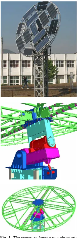
The system of orientation is done for a column on which is put through two cinematic joints a platform with shape like a disk where solar panels (Figure 1) are fixed. The disk on which the solar panels are fixed has two degrees of freedom (Figure 1).
2. Material and Methods
For action whole system on two degrees of freedom are used a hydraulic group which actions two hydraulic motors one rotary and the other linear. The main purpose of the two degrees of freedom disk is to obtain the best energetic conversion of solar energy into electrical energy. Because the system of orientation works in an environment where there are many variations like wind speed, seismic loads, temperature variations, it is necessary to
design a compensator for position of orientation like PD controllers. System of control disposes of many digital and analogue input and output, a part of this inputs and outputs are used for different procedures. Because the speed of wind is very large owing to environment where the structure is placed, there is a procedure to reduce the surface exposed on direction of wind that bring the structure in a control position. There are also procedures that allow recording all information about capacity of conversion of solar energy in electrical energy and reliable working of hydraulic system.
The main movement is made in steps considering that the solar hour has 15°. In order to have an incidence angle normal to the solar panels plan, a higher period of time the daily rotation takes place by adopting a displacement law which during on 15° cross the steps acceleration - steady state - deceleration. Therefore the main
movement takes place considering the displacement law on periods of 15°. After finishing a stage between +80° and –80° the orientation system of solar panels is taken in the start position by rotating counter clockwise with one rotation of 160°.
The seasonal rotation movement which depends on the season takes place between 0° and 45° and it is perpendicular on the main rotation movement. Because this movement is made between big periods of time and is not necessary a high accuracy of positioning we decide that for this degree of freedom to not perform the displacement control of orientation system of solar panels. During the execution of seasonal rotation, the accelerations that appear are small due to the fact that de periods of acceleration and deceleration are done in long period of time. Clearly that the range of variation of inertia at the rotation movement around the main axis is very big because for each position between 0° and 45° in the secondary rotation couple, the disc on which are fixed the solar panels execute the main rotation movement between +80° and –80°.
One of the problems that occur at the construction of this kind of structure is the transitory response of structure at acceleration and deceleration of system, due to the fact that for one complete movement are necessary, on average, 18 accelerations and decelerations of driving system during one day in the main couple of rotation [3].
2.1. Dynamic model for system with two degrees of freedom and controller PID
For the dynamic model in this paper the author considers that concentrated mass and element of the system are rigid elements. The bodies that compose the system can be considered rigid bodies because when the column and disk for system of orientation solar panel was designed, complex modal analysis for all components of structure was
Fig. 1. The structure having two cinematic degrees of freedom positioned on the
performed. Period for all components of
structure is T < 0.2 s, in this way all components can be considered as rigid bodies [1] (Figure 2).
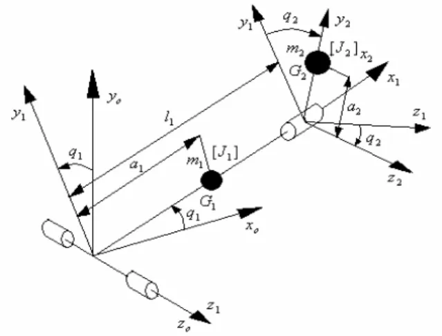
Fig. 2. Dynamic model - for a system with two degrees of freedom with concentrated masses and rigid elements
Cinematic parameters-position angular speed and angular acceleration for mass m2 and m1 are: - position: ; 0 0 , 0 1 1 2 1 2 ⎪ ⎭ ⎪ ⎬ ⎫ ⎪ ⎩ ⎪ ⎨ ⎧ = ⎪ ⎭ ⎪ ⎬ ⎫ ⎪ ⎩ ⎪ ⎨ ⎧ = a r a l r (1) - angular speed: ; 0 0 , cos sin 1 1 2 1 2 1 2 2 ⎪ ⎭ ⎪ ⎬ ⎫ ⎪ ⎩ ⎪ ⎨ ⎧ = ω ⎪ ⎭ ⎪ ⎬ ⎫ ⎪ ⎩ ⎪ ⎨ ⎧ = ω q q q q q q & & & & (2) - angular acceleration: ; 0 0 , sin cos cos sin 1 1 2 2 1 2 1 2 2 1 2 1 2 2 ⎪ ⎭ ⎪ ⎬ ⎫ ⎪ ⎩ ⎪ ⎨ ⎧ = ε ⎪ ⎭ ⎪ ⎬ ⎫ ⎪ ⎩ ⎪ ⎨ ⎧ − + = ε q q q q q q q q q q q q && & & && & & && && (3) - linear speed: . sin cos cos , 0 0 2 2 2 1 1 2 1 1 2 2 1 2 1 1 1 ⎪ ⎭ ⎪ ⎬ ⎫ ⎪ ⎩ ⎪ ⎨ ⎧ + − − = ⎪ ⎭ ⎪ ⎬ ⎫ ⎪ ⎩ ⎪ ⎨ ⎧ = q q q l q q l q q a q v a q v & & & & & (4)
Kinetic energy for body with mass m1 is: . ) ( 2 1 1 2 1 1 2 1 1 q ma J z E = & + (5)
Kinetic energy for body with mass m2 is:
. sin ) ( 2 1 ) cos cos sin ( 2 1 2 2 2 1 2 1 2 2 2 2 2 2 2 1 2 2 2 2 2 2 2 2 2 2 2 2 2 1 2 m q a l q q a m J q l m q a m q J q J q E x z y & & & & − + + + + + =
Gravitational energy for body with mass m1 is:
Gravitational energy for body with mass m2 is: . ) cos cos sin (1 1 2 2 1 2 2 m g l q a q q U = +
Generalized force that actions in the joints of the structure are obtained through Lagrange equations: 2 . 1 ; = = ∂ ∂ − ⎟ ⎟ ⎠ ⎞ ⎜ ⎜ ⎝ ⎛ ∂ ∂ q k Q k q L k q L dt d & , (7)
where: L - langrangean for system of two bodies; qk - generalized coordinate; q&k - generalized velocity; Qk - generalized force that actions in the joints of structure.
Generalized force that actions in the first joint: . ) cos sin cos ( cos cos sin ) ( 2 cos sin )) cos ( cos sin ( 2 1 2 1 1 2 1 1 1 2 2 2 2 2 2 2 2 1 2 2 1 2 2 2 2 2 2 1 2 2 2 1 2 2 2 2 2 2 1 1 2 2 2 2 2 2 1 1 1 q q a q l g m q ga m q q a m J J q q q a l m q q q a l m q l q a m a m q J q J J q Q z y z y z z − − − − − + − − + + + + + = & & & && &&
Generalized force that actions in second joint: . sin cos cos sin ) ( ) ( sin 2 1 2 2 2 2 2 2 2 2 2 2 1 2 2 2 2 2 2 2 2 1 2 1 2 q q ga m q q a m J J q a m J m q q a l m q Q z y z x + − − − + + − = & && &&
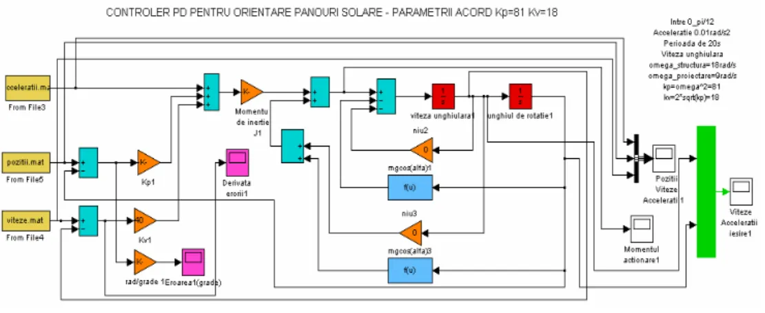
The scheme for the PD controller used to control the two degrees of freedom system is presented in Figure 3.
The PD controller [2] was designed based on the law of momentum calculus. The
momentum value, generated by the PD controller designed in Simulink. In order to determine Kp and Kv constants, the following scheme was realized (Figure 3). Movement laws in displacement, velocity and acceleration were imported from MATLAB program (Figure 4a):
, ) ( ) ) ( ) ( )( ( τ , ) ( ) ( , ) ( ) )( ( τ q q, N e k diag k diag q q M e k diag e k diag u q q, N u q q M Pi Vi d Pi Vi d & && & & && + + + = − − = + − = (8)
where, τ the vector of generalized moments in the couple; M(q) is the system’s matrix of inertia; N(q,q&) is the nonlinear terms vector; q&&d is the designed accelerations vector; diag(kVi) the diagonal matrix formed by the controller derivative tune parameters; diag(kPi) the diagonal matrix formed by the controller proportional tune parameters; e is the errors vector; e& is the velocity errors vector.
The error variation law in the case of the PD controller is represented in Figure 4b:
, τ ) ( ) ( ) ( , τ ) ( ) ( τ , ) ( ) ) ( ) ( )( ( τ 1 p Pi Vi p Pi Vi d q M e k diag e k diag e q q, N q q M q q, N e k diag k diag q q M − = + + + + = + + + = & && & && & && (9)
where, q&& is the vector of measurable accelerations in the couple; τp is the vector of disturbing moments.
The tune parameters of the PD controller are determined form the condition as the system to be critically damped:
. ω ; 2 1 ς , ω ; ςω 2 2 2 p p p V p p p V k k k k k = = ⇒ = = = (10)
Fig. 3. PD control for one degree of freedom for the orientating solar panels structure
Fig. 4a. Acceleration, velocity, displacement-controller PD
Fig. 4b. Positioning error-controller PD Increasing the ωp frequency, leads to decreasing the perturbation M−1(q)τ
p, which has to be rejected. The value of ωp must be superior limited in order to avoid the
resonance phenomena at ωp = ωs/2, where
ωs is the own frequency of the structure. The biggest imprecision from the movement law are in the accelerating and decelerating periods of the system due to inertia forces.
3. Conclusions
• Configuration of the stiffness structure for the pylon as for the platform on which the solar panels are fixed was done in order to minimize the relative displacements. Considering small displacements it yields that the elements of the structure can be considered rigid, in this way the dynamic degrees of freedom are becoming important.
• In order to consider the orientating structure as being composed of rigid bodies, the own period of the structure’s elements was under 0.2 s.
• Because on the first dynamic degree of freedom the movement is rare and the movement law in acceleration, velocity and displacement does not imply a significant variation of the action force on the second degree of freedom, in order to improve the control parameters a dynamic model with a single degree of freedom was considered, the one that the movement during the day takes place.
• PD control in position for the platform allowed increasing the positioning precision in order to maximize the overall energetic efficiency.
• For the case in which wind acts perpendicular on the platform, a procedure was created to reduce the exposed surface by orientating the platform parallel to the ground. In order to consider also in this case the two degree of freedom system as a single cinematic degree of freedom system, the movements are successive done on each cinematic degree of freedom.
• By analyzing the obtained results, it yields that the smallest positioning error is obtained in the case of PD controller having optimized tune parameters.
• In order to advance the positioning
precision, one can consider increasing the orientating structure’s elements stiffness by a proper configuration.
References
1. Botiş, M.: Metoda elementului finit (The Finite Element Method). Cluj Napoca. Napoca Star Publishing House, 2010.
2. Ogata, K.: Modern Control Engineering. 5th Edition. New Jersey. Pretince-Hall, 2009.
3. Sorensen, A.J.: A Survey of Dynamic Positioning Control Systems. In: Annual Reviews in Control 35 (2011) Issue 1, p. 123-136.