Deposited in DRO:
23 April 2015
Version of attached le:
Published Version
Peer-review status of attached le:
Peer-reviewed
Citation for published item:
Liu, J. and Hennig, C. and Desai, S. and Hoyle, B. and Koppenhoefer, J. and Mohr, J. J. and Paech, K. and Burgett, W. S. and Chambers, K. C. and Cole, S. and Draper, P. W. and Kaiser, N. and Metcalfe, N. and Morgan, J. S. and Price, P. A. and Stubbs, C. W. and Tonry, J. L. and Wainscoat, R. J. and Waters, C. (2015) 'Optical conrmation and redshift estimation of the Planck cluster candidates overlapping the Pan-STARRS Survey.', Monthly notices of the Royal Astronomical Society., 449 (4). pp. 3370-3380.
Further information on publisher's website:
http://dx.doi.org/10.1093/mnras/stv458Publisher's copyright statement:
This article has been accepted for publication in Monthly notices of the Royal Astronomical Society. c: 2015 The
Authors Published by Oxford University Press on behalf of the Royal Astronomical Society. All rights reserved. Additional information:
Use policy
The full-text may be used and/or reproduced, and given to third parties in any format or medium, without prior permission or charge, for personal research or study, educational, or not-for-prot purposes provided that:
• a full bibliographic reference is made to the original source • alinkis made to the metadata record in DRO
• the full-text is not changed in any way
The full-text must not be sold in any format or medium without the formal permission of the copyright holders. Please consult thefull DRO policyfor further details.
Durham University Library, Stockton Road, Durham DH1 3LY, United Kingdom Tel : +44 (0)191 334 3042 | Fax : +44 (0)191 334 2971
Optical confirmation and redshift estimation of the
Planck
cluster
candidates overlapping the Pan-STARRS Survey
J. Liu,
1,2‹C. Hennig,
1,2‹S. Desai,
1,2B. Hoyle,
1J. Koppenhoefer,
1,3J. J. Mohr,
1,2,3‹K. Paech,
1W. S. Burgett,
4K. C. Chambers,
4S. Cole,
5P. W. Draper,
5N. Kaiser,
4N. Metcalfe,
5J. S. Morgan,
4P. A. Price,
6C. W. Stubbs,
7J. L. Tonry,
4R. J. Wainscoat
4and C. Waters
41Department of Physics, Ludwig-Maximilians-Universit¨at, Scheinerstr. 1, D-81679 M¨unchen, Germany 2Excellence Cluster Universe, Boltzmannstr. 2, D-85748 Garching, Germany
3Max-Planck-Institut f¨ur extraterrestrische Physik, Giessenbachstr., D-85748 Garching, Germany 4Institute for Astronomy, University of Hawaii at Manoa, Honolulu, HI 96822, USA
5Department of Physics, Durham University, South Road, Durham DH1 3LE, UK 6Department of Astrophysical Sciences, Princeton University, Princeton, NJ 08544, USA 7Department of Physics, Harvard University, Cambridge, MA 02138, USA
Accepted 2015 March 2. Received 2015 January 30; in original form 2014 July 22
A B S T R A C T
We report results of a study of Planck Sunyaev–Zel’dovich effect selected galaxy cluster candidates using the Panoramic Survey Telescope & Rapid Response System (Pan-STARRS) imaging data. We first examine 150Planck-confirmed galaxy clusters with spectroscopic redshifts to test our algorithm for identifying optical counterparts and measuring their redshifts; our redshifts have a typical accuracy ofσz/(1+z) ∼0.022 for this sample. Using 60 random
sky locations, we estimate that our chance of contamination through a random superposition is∼3 per cent. We then examine an additional 237Planckgalaxy cluster candidates that have no redshift in the source catalogue. Of these 237 unconfirmed cluster candidates we are able to confirm 60 galaxy clusters and measure their redshifts. A further 83 candidates are so heavily contaminated by stars due to their location near the Galactic plane that we do not attempt to identify counterparts. For the remaining 94 candidates, we find no optical counterpart but use the depth of the Pan-STARRS1 data to estimate a redshift lower limitzlim(1015)beyond which
we would not have expected to detect enough galaxies for confirmation. Scaling from the already publishedPlancksample, we expect that∼12 of these unconfirmed candidates may be real clusters.
Key words: catalogues – galaxies: clusters: general – large-scale structure of Universe.
1 I N T R O D U C T I O N
Massive clusters of galaxies sample the peaks in the dark matter den-sity field, and analyses of their existence, abundance and distribu-tion enable constraints on cosmological parameters and models (e.g. White, Efstathiou & Frenk1993; Eke, Cole & Frenk1996; Vikhlinin et al.2009; Mantz et al.2010; Rozo et al.2010; Williamson et al.
2011; Hoyle et al.2012; Mana et al.2013; Bocquet et al.2015). Surveys at mm wavelengths allow one to discover galaxy clusters through their Sunyaev–Zel’dovich effect (Sunyaev–Zel’dovich ef-fect (SZE)), which is due to inverse Compton interactions of cosmic
E-mail:[email protected](JL);[email protected](CH);
[email protected](JJM)
microwave background (CMB) photons with the hot intracluster plasma (Sunyaev & Zel’dovich1970,1972). Since the first SZE-discovered galaxy clusters were reported by the South Pole Tele-scope (SPT) collaboration (Staniszewski et al.2009), large solid angle surveys have been completed, delivering many new galaxy clusters (Hasselfield et al.2013; Reichardt et al.2013; Planck Col-laboration XXIX2014a).
The SZE observations alone do not enable one to determine the cluster redshift, and so additional follow-up data are needed. In previous X-ray surveys, it was deemed necessary to obtain initial imaging followed by measurements of spectroscopic redshifts for each cluster candidate (e.g. Rosati et al.1998; B¨ohringer et al.2004; Mehrtens et al.2012). In ongoing SZE surveys, the efforts focus more on dedicated optical imaging (e.g. Song et al.2012b; Planck Collaboration XXIX2014a) to identify the optical counterpart and
measure photometric redshifts. In the best case, one leverages existing public wide field optical surveys such as the Sloan Digital Sky Survey (York et al.2000), the Red Sequence Cluster Survey (Gladders & Yee2005) or the Blanco Cosmology Survey (Desai et al.2012).
In 2013 March the Planck Collaboration released an SZE source catalogue with 1227 galaxy cluster candidates from the first 15 months of survey data Planck Collaboration XXIX (2014a). Given the full-sky coverage of thePlancksatellite, there is no sin-gle survey available to provide confirmation and redshift estimation for the full candidate list. Of this full sample, 683 SZE sources are associated with previously known clusters (e.g. Meta-Catalogue of X-ray-detected Clusters of galaxies, Piffaretti et al.2011; MaxBCG catalogue, Koester et al.2007; GMBCG catalogue, Hao et al.2010; AMF catalogue, Szabo et al.2011; WHL12 catalogue, Wen, Han & Liu 2012; and SZ catalogues from Williamson et al. 2011; Hasselfield et al.2013; Reichardt et al. 2013) and 178 are con-firmed as new clusters, mostly through targeted follow-up obser-vations. The remaining 366 SZE sources are classified into three groups depending on the probability of their being a real galaxy cluster.
In this paper, we employ proprietary Panoramic Survey Telescope & Rapid Response System (Pan-STARRS) imaging data and a blinded analysis (Klein & Roodman2005) to perform optical cluster identification and to measure photometric redshifts ofPlanck
cluster candidates. For those candidates where no optical counter-part is identified, we provide redshift lower limits that reflect the limited depth of the optical imaging data.
This paper is organized as follows: we briefly describe the SZE source catalogue in Section 2.1 and the optical Pan-STARRS data processing in Section 2.2. In Section 3, we provide the details of the photometric redshift (photo-zhereafter) estimation and cluster confirmation pipeline. Results of the photometric redshift (photo-z) performance and the confirmation ofPlanck candidates are pre-sented in Section 4.
2 DATA D E S C R I P T I O N
We briefly describe thePlanckSZE source catalogue in Section 2.1 and refer the reader to the cited papers for more details. In Section 2.2, we then describe the Pan-STARRS optical data and calibration process we use to provide the images and calibrated catalogues needed for the cluster candidate follow up.
2.1 PlanckSZE source catalogue
ThePlanckSZE source catalogue contains 366 unconfirmed clus-ter candidates, and it is available for download.1This catalogue
is described in detail elsewhere (see Planck Collaboration XXIX
2014a). In summary, the Planck SZE sources are the union of detections from three independent pipelines, which are compared extensively in Melin et al. (2012). The pipelines, which are op-timized to extract the cluster SZE signal from thePlanckCMB data, are drawn from two classes of algorithms, namely two matched-multifilter pipelines, which are multifrequency matched filter approaches Melin, Bartlett & Delabrouille (2006), and the PowellSnakes pipeline, which is a fast Bayesian multifrequency detection algorithm Carvalho et al. (2012).
1http://pla.esac.esa.int/pla/
The ‘union sample’ is the combination of detections from each of these three pipelines with a measured signal-to-noise ratio (SNR) above 4.5. Detections are further merged if they are within an an-gular separation of≤5 arcmin. The detection, merging and combi-nation pipelines have been tested using simulations and achieve a purity of 83.7 per cent Planck Collaboration XXIX (2014a). With a sample of 1227 cluster candidates, we estimate that approximately 200 (∼1227×(1–83.7 per cent)) are noise fluctuations. Thus, we expect to find 200 false detections in the remaining 366 unconfirmed candidates, indicating that the probability of an unconfirmed candi-date to be a bona fide cluster is only (1−200/366)∼45 per cent. The candidates in the union sample are grouped into three clas-sification levels according to the likelihood of being a cluster. Class 1 is for high-reliability candidates that have a good detec-tion in the SZE and are also associated withROSATAll Sky Survey (RASS; Voges et al.1999) andWide-field Infrared Survey Explorer
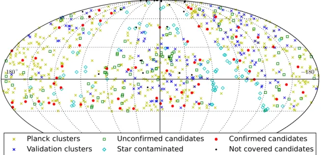
(WISE; Wright et al.2010) detections. The Class 2 candidates meet at least one of the three criteria in Class 1. The Class 3 candidates correspond to low-reliability candidates that have poor SZE detec-tions and no clear association withROSATAll Sky Survey (RASS) orWide-field Infrared Survey Explorer(WISE) detections. A total of 237 unconfirmedPlanckcluster candidates (Classes 1, 2 and 3) lie within the Pan-STARRS footprint with enough coverage (cf. Fig.1
and Section 2.2.1).
The union sample also contains redshifts for previously known and confirmed clusters. We create a validation sample by randomly selecting 150 of these clusters that fall within the Pan-STARRS footprint and have quotedPlanckredshift uncertainties of<0.001. We combine these 150 confirmed clusters with the sample of 237 cluster candidates for a total sample of 387 clusters and candidates. We subject all targets in our total sample to the same procedure. This blind analysis of our optical confirmation and photo-zestimation pipelines enables an important test of our methods as well as the characterization of our photometric redshift uncertainties. Note that the heterogeneous nature ofPlanckconfirmation may result in a different redshift and mass distribution of the validation sample from that of unconfirmed clusters, but we do not expect this to lead to any important bias. In what follows, we refer to both confirmed clusters and cluster candidates within this total combined sample as ‘candidates’.
For each candidate we use the following additional information given by each of the three individual SZE detection pipelines: the candidate position (right ascensionα, declinationδ), the position uncertainty, the best-estimated angular size (θs), and the integrated
SZE signal YSZ from the θs–YSZlikelihood plane provided with
thePlanckdata products. Furthermore, we convert the size to an angular estimate ofθ500 =c500θs, where the concentration is set
toc500 =1.177 as used in the cluster detection pipelines Planck
Collaboration XXIX (2014a). This angular radiusθ500corresponds
to the projected physicalR500within which the density is 500 times
the critical density at the redshift of the cluster. In Fig.2, we show theYSZ–θ500distribution of the combined sample used in this work.
2.2 PAN-STARRS1 data
For each candidate, we retrieve the single-epoch detrended images from the Pan-STARRS1 (PS1) data server and use those data to build deeper coadd images in each band. This involves cataloguing the single-epoch images, determining a relative calibration, combining them into coadd images, cataloguing the coadds and then determin-ing an absolute calibration for the final multiband catalogues. We describe these steps further below.
Figure 1. The sky distribution ofPlanckclusters and candidates within the PS1 region. The crosses are previously confirmedPlanckclusters, and the blue crosses mark the validation sample we use in this analysis. For the remainder of the sample of previously unconfirmedPlanckcandidates, black dots mark those that are not fully covered by PS1 data, red circles are clusters we confirm (see Table2), cyan diamonds are candidates that lie in areas of heavy star contamination, and green squares are candidates we do not confirm (see Table3).
2.2.1 Data retrieval
The Pan-STARRS Kaiser et al. (2002) data used in this work are obtained from a wide field 1.8 metre telescope situated on Haleakala, Maui in Hawaii. The PS1 telescope is equipped with a 1.4 gigapixel CCD covering a 7 deg2field of view, and it is being used in the
PS1 survey to image the sky north ofδ= −30◦. The 3πsurvey is so named because it covers 75 per cent of the celestial sphere. The PS1 photometric system is similar to the Sloan Digital Sky Survey (SDSS) filter system withgP1,rP1,iP1,zP1,yP1(where SDSS hadu),
and a wide bandwP1for use in the detection of Near Earth Objects
Tonry et al. (2012). In this study, we process data from the first four filters and denote them asgriz.
We obtain single-epoch, detrended, astrometrically calibrated and warped PS1 imaging data (Metcalfe et al.2013) using the PS1 data
Figure 2. TheYSZ–θ500distribution ofPlanckclusters and candidates in our sample. ThePlanckconfirmed clusters are shown with blue crosses, and the six cases where our pipeline failed to confirm the systems are marked with black stars (see Section 4 for more details). ThePlanckcandidates with Pan-STARRS1 (PS1) data are shown with red circles if we are able to measure a corresponding photometric redshift and with green squares if not.
access image server. We use 3PI.PV2 warps wherever available and 3PI.PV1 warps in the remaining area. We select those images that overlap the sky location of each candidate, covering a square sky region that is∼1◦on a side. The image size ensures that a sufficient area is available for background estimation.
2.2.2 Single-epoch relative calibration
The subsequent steps we follow to produce the science ready coadd images and photometrically calibrated catalogues are carried out us-ing the Cosmology Data Management system (CosmoDM), which has its roots in the Dark Energy Survey data management system (Ngeow et al.2006; Mohr et al.2008,2012) and employs several AstrOMatic codes that have been developed by Emmanuel Bertin (Institut d’Astrophysique de Paris).
We build catalogues from the PS1 warped single-epoch images using SEXTRACTOR(Bertin & Arnouts1996). The first step is to
pro-duce a model of the point spread function (PSF) variations over each of the input single-epoch images. This requires an initial catalogue containing stellar cutouts that are then built, usingPSFEX(Bertin
2011), into a position dependent PSF model. With this model we then recatalogue each image using model fitting photometry with the goal of obtaining high-quality instrumental stellar photometry over each input image.
For each band, relative photometric calibration is performed using these catalogues; we compute the average magnitude dif-ferences of stars from all pairs of overlapping images and then determine the relative zeropoints using a least squares solu-tion. The stars are selected from the single-epoch catalogues us-ing the morphological classifierspread_model (e.g. in particu-lar |spread model|<0.002; see Desai et al. 2012; Bouy et al.
2013). We use the PSF fitting magnitudemag_psffor this relative calibration.
We test the accuracy of the single-epoch model fitting relative photometry by examining the variance of multiple, independent
Figure 3. The left-hand panel shows the histogram of single-epoch repeata-bility scatter, extracted for bright stars in the full ensemble of candidates. All bands have similar distributions, and so only the combined distribution is shown. The median scatter is 16, 18, 19 and 17 mmag ingriz, respec-tively. The right-hand panel shows the histogram of the stellar locus scatter extracted from the full ensemble of 387 candidates. The median values of the scatter distributions for all candidates are 34, 24 and 57 mmag ing−r
versusr−i,r−iversusi−zandg−rversusr−Jcolour spaces.
measurements of stars. Fig.3contains a histogram of the so-called repeatability of the single-epoch photometry. These numbers cor-respond to the root-mean-square (rms) variation of the photometry of bright stars scaled by 1/√2, because this is a difference of two measurements. We extract these measurements from the bright stars where the scatter is systematics dominated (i.e. the measurement uncertainties make a negligible contribution to the observed scatter). We measure this independently for each band and candidate and use the behaviour of specific candidate tiles relative to the ensemble to identify cases where the single-epoch photometry and calibration need additional attention. The median single-epoch repeatability scatter is 16, 18, 19 and 17 mmag ingriz, respectively.
As part of this process we obtain PSF full width at half-maximum (FWHM) size measurements for all single-epoch images. The me-dian FWHM for the full ensemble of imaging over all cluster can-didates is 1.34, 1.20, 1.12 and 1.09 arcsec ingriz, respectively.
2.2.3 coaddition, cataloguing and absolute calibration
The coadd images are then generated from the single-epoch im-ages and associated relative zeropoints. For each candidate tile we generate both PSF homogenized and non-homogenized coadds. To create the homogenized coadds, we convolve the input warp im-ages to a PSF described by a Moffat function with FWHM set to equal the median value in the single-epoch warps overlapping that candidate. We homogenize separately for each band. We then com-bine these homogenized and non-homogenized warps usingSWARP
(Bertin et al.2002) in a median combine mode. We create aχ2
detection image (Szalay, Connolly & Szokoly1999) from the ho-mogenized coadds using bothiandzbands. The PSF-homogenized coadds are then catalogued using SEXTRACTORin dual image mode
with thisχ2detection image. We use SE
XTRACTORin PSF
correct-ing, model fitting mode. The non-homogenized coadds are only used for visual inspection and for creating pseudo-colour images of the candidates (see Fig.4). For a more detailed discussion of coadd homogenization on a different survey data set, see Desai et al. (2012).
We use the stellar locus together with the absolute photometric calibration from the 2MASS survey (Skrutskie et al.2006) for the final, absolute photometric calibration for our data (see also Desai
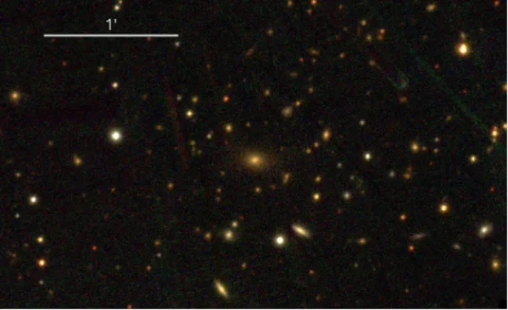
Figure 4. Example pseudo-colour image in thegribands of cluster candi-date 218. In this case, thePlanckSZE candidate centre is about 4 arcmin away from the Brightest Cluster Galaxy (BCG), which is at the centre of this image. This exemplifies an extreme case of the large offset between the
Planckcentre and the BCG.
et al.2012, and references therein). For this process, we adopt the PS1 stellar locus measured by Tonry et al. (2012).
In our approach, we first apply extinction corrections to the rel-ative photometry from the catalogues using the dust maps from Schlegel, Finkbeiner & Davis (1998). This correction removes the overall Galactic extinction reddening, making the stellar locus more consistent as a function of position on the sky. As is clear from Fig.1, thePlanckcluster candidates extend to low galactic latitude, and some lie in locations of extinction as high asAV=1.8 mag.
Most of the targets withAV>0.5 mag also have very high
stel-lar contamination, making it impossible for us to use the PS1 data for candidate confirmation. High et al. (2009) examined photomet-rically calibrated data lying in regions with a range of extinction reaching up to AV∼ 1 mag, showing that within this range the
stellar locus inferred shifts are equivalent to the Galactic extinction reddening corrections to within an accuracy of∼20 mmag.
We then determine the best-fitting shifts ing−randr−ithat bring our observed stellar sample to coincide with the PS1 locus. We repeat this procedure fori−zwhile using ther−iresult from the previous step. This allows for accurate colour calibration for the PS1 bands used for the cluster photometric redshifts. To obtain the absolute zeropoint, we adjust theg−rversusr−Jlocus until it coincides with the PS1 locus. This effectively transfers the∼2 per cent 2MASS photometric calibration (Skrutskie et al.2006) to our PS1 catalogues.
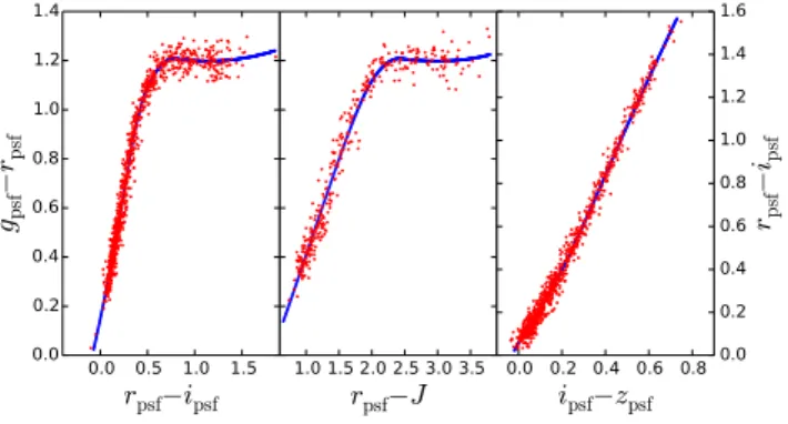
An illustrative plot of the stellar loci forPlanckcluster 307 is shown in Fig.5. The scatter of our model fitting photometry about the stellar locus provides a measure of the accuracy of the coadd model fitting photometry. In the case of candidate 307, the scatter around the stellar locus ing−rversusr−i,g−rversusr−Jand
r−iversusi−zis 29, 48 and 17 mmag, respectively. In Fig.3, we show the histogram of scatter for the ensemble of candidates in each of these colour–colour spaces. The median scatter of the stellar locus is 34, 24 and 57 mmag ing−rversusr−i,r−iversusi−z
andg−rversusr−J, respectively. These compare favourably with the scatter obtained from the SDSS and BCS data sets (Desai et al.
2012). Note that the shallow 2MASS photometry contributes sig-nificantly to the scatter in one colour–colour space, but in the others we restrict the stars to only those with photometric uncertainties
<10 mmag (see Fig.3). We use the scatter measurements within each candidate tile together with the behaviour of the ensemble to identify any candidates that require additional attention. We note
Figure 5. The stellar loci in three different colour–colour spaces for the
Planckcluster 307 are shown. The blue line shows the PS1 stellar locus, and red points show PSF model fitting magnitudes of stars from our catalogues for this tile. We use the stellar locus for absolute photometric calibration. The scatter about the stellar locus provides a good test of photometric quality; for this cluster the values of the scatter ing−rversusr−i(left),g−r
versusr−J(middle) andr−iversusi−z(right) colour spaces are 29, 48 and 17 mmag, respectively.
that the PS1 ubercal calibration method (Schlafly et al.2012) has been able to achieve internal photometric precision of<10 mmag in photometric exposures ing,randiand10 mmag inz, but it has not been applied over the whole 3PI data set yet.
We estimate a photometric 10σ depth, above which the galaxy catalogue is nearly complete, in each coadd by calculating the mean magnitude of galaxies withmag_autouncertainties of 0.1. In Fig.6, we show the histograms of the distribution of depths in each band; the median depths ingrizare 20.6, 20.5, 20.4 and 19.6 (de-noted by dotted lines). We note that the median depths are shallower than the limiting depths reported by the PS1 collaboration Metcalfe et al. (2013), but this difference is mainly due to a different definition of the depth. We find that to this depth the magnitude measurements frommag_autoand the colour measurements usingdet_modelare well suited for the redshift estimation analysis which we describe in Section 3.2.
Variation in observing conditions leads to non-uniform sky cov-erage across the PS1 footprint. One result is that the depth varies
Figure 6. The distributions ofgrizband 10σdepths (mag_auto) for PS1 fields around eachPlanckcandidate. The dashed lines mark the magnitudes ofLgalaxies at different redshifts. The dotted lines mark the median depths, which are 20.6, 20.5, 20.4 and 19.6 ingriz, respectively. The PS1 data are typically deep enough for estimating cluster redshifts out to or just beyond
z=0.5 (see also Fig.8).
considerably from candidate to candidate; another is that not all candidates are fully covered in each of the bands of interest. Over-all 387 cluster candidates have been fully covered. In Fig.1, we show the sky distribution of our full sample together with that of thePlancksample.
3 M E T H O D
In this section, we describe the optical confirmation and redshift estimation technique that we apply to the PS1 galaxy catalogues (see Section 3.1). Then in Section 3.2, we describe the method we use – especially in candidates without optical counterparts – to estimate the redshift lower limit as a function of the field depth.
3.1 Confirmation and redshift estimation
We employ the red sequence galaxy overdensity associated with a real cluster to identify an optical counterpart for thePlanck candi-dates and to estimate a photometric redshift; our method follows closely that of Song et al. (2012a), which has been applied within the SPT collaboration to confirm and measure redshifts for 224 SZE-selected cluster candidates (Song et al.2012b) and then later for the full 2500 deg2SPT-SZ survey sample (Bleem et al.2015).
A similar approach has been used to identify new clusters from opti-cal multiband surveys using only the overdensity of passive galaxies with similar colour (Gladders & Yee2005). We start with additional information from the SZE or X-ray about the sky location and, in principle, also a mass observable such as the SZE or X-ray flux that can be used at each redshift probed to estimate the cluster mass and characterize the scale of the virial region within which the red sequence search is carried out (Hennig et al., in preparation). We describe the procedure below.
We model the evolutionary change in colour of cluster member galaxies across cosmic time by using a composite stellar population model initialised with an exponentially decaying starburst starting at redshiftz=3 with decay timeτ=0.4 Gyr (Bruzual & Charlot
2003). We introduce tilt into the red sequence of the passive galax-ies by adopting six models with different metallicitgalax-ies adjusted to follow the observed luminosity–metallicity relation in Coma (Poggianti et al.2001). Using the absolute PS1 filter transmission curves, which include atmospheric, telescope and filter corrections (Tonry et al.2012), as inputs for the packageEZGAL(Mancone & Gonzalez2012), we generate fiducial galaxy magnitudes in griz
bands over a range of redshifts and within the range of luminosities 3L≥L≥0.3L, whereLis the characteristic luminosity in the Schechter (1976) luminosity function.
We exclude faint galaxies by employing a minimum magnitude cut of 0.3L; to reduce the number of junk objects in the catalogue we remove all objects with a magnitude uncertainty>0.3. In Song et al. (2012b), a fixed aperture is used to both select cluster galax-ies and perform background subtraction. In this work, we use the
Planck-derived radiusθ500centred on the position of the candidate
to separate galaxies into cluster and field components. Galaxies lo-cated within the range (1.5–3)θ500are used to estimate background
corrections. Each galaxy within the radial apertureθ500is assigned
two weighting factors. The first one is a Gaussian colour weighting corresponding to how consistent the colours of the galaxy are with the modelled red sequence at that redshift. This red likelihood,Lred,
is calculated separately for each of the following colour combina-tions:g−randg−i, which are suitable for low-redshift (z <0.35) estimation, andr–iandr−z, which are suitable for intermediate-redshift (0.35< z <0.7) estimation. The second factor weights the
galaxy depending on the radial distance to the cluster centre,Lpos,
and for this function we adopt a projected NFW profile Navarro, Frenk & White (1997) with concentrationc=3. In this way, all galaxies physically close to the cluster centre and with colours con-sistent with the red sequence at the redshift being probed are given higher weight. Conversely, any galaxies in the cluster outskirts with colours inconsistent with the red sequence are given a small weight. The method then scans a redshift range 0< z <0.7 with an intervalδz = 0.01 and iteratively recomputes the above weight factors using the modelled evolution of the red sequence. For each cluster candidate, we construct histograms of the weighted number of galaxies as a function of redshift for each above-mentioned colour combination. The weighted number of galaxies is determined for each colour combination as the background subtracted sum of all galaxy weights at each given redshift.
For each cluster, we identify the appropriate colour combination using a visual examination of the red sequence galaxies within the cluster centre and record the BCG position, if possible. The final photo-zis estimated by identifying the most significant peak in the background-corrected likelihood histogram from all galaxies withinθ500. The associated photo-zuncertainty is determined from
the width of a Gaussian fit to the peak with outliers at>3σremoved. Specifically, the photo-zuncertaintyδzphotis the standard deviation
of the Gaussian divided by the square root of the weighted galaxy number in the peak. The performance is presented in the following section. We note that, given the depth of the data (see Fig.6), we are unable to identify candidates with redshiftsz >0.7.
The optical confirmation and photo-zestimation break down if no significant peak is found in the likelihood histogram. In addition to the case where the candidate is not a cluster, there are three categories of failure that are possible: (1) those candidates with aPlanckθ500 that is so small such that there are not enough red
sequence galaxies within the search aperture, (2) those that have a radiusθ500above 30 arcmin, in which case our standard 0◦.7×0◦.7
coadd catalogue region typically does not contain enough remaining area to measure the background well and (3) those candidates that have a relatively large offset between the visually confirmed cluster centre and thePlanckposition. Clusters withθ500>30 arcsec all
lie at low redshift, where – given the sensitivity of thePlanckSZE selection – we would expect these systems to have already have been confirmed by low-redshift all sky surveys (e.g. Abell1958; Abell, Corwin & Olowin1989; Voges et al.1999). For cases 1 and 2, we rerun the pipeline with a radius of 5 arcmin, which is the same as thePlanckmatching radius. For the third case, we recentre at the coordinates of the BCG if a BCG can be identified within the coadd region. With the approach described above, the uncertainties associated with the Planck candidate position and size have no significant impact on our confirmation and photo-zestimation. We demonstrate this with the validation sample in Section 4.1.
3.2 Redshift lower limitszlim(1015)
For clusters where there is no obvious overdensity of red sequence galaxies, there are two possibilities: (1) the candidate is a noise fluctuation, or (2) the cluster is at high enough redshift that the PS1 imaging data is not deep enough to detect the cluster galaxy pop-ulation. Given the contamination estimates provided by thePlanck
collaboration, we expect approximately half of our candidates to be noise fluctuations. However, of the 45 per cent that are real clusters we expect a small fraction of them to lie at redshifts too high to be followed up using the PS1 data. In particular, the observed redshift distribution of the 813 previously confirmedPlanckclusters has
3 per cent of those clusters lying atz >0.60, which is a reasonable expectation of the redshift limit to which we could expect to use PS1 data to confirm a cluster. Simple scaling suggests we should expect approximately 3 clusters to lie atz >0.6 in our candidate sample. Thus, for each of these undetected systems we calculate the minimum redshiftzlim(1015) beyond which the candidate would be
undetectable in our PS1 imaging.
To estimate the redshift lower limit we first measure the depth of the catalogue at the coordinates of the candidate (see Fig.6) and then predict, as a function of redshift, the statistical significance of the detectable galaxy overdensity above background. To do this we adopt a typical mass for aPlanckcluster ofM200=1×10¹⁵M
and use a model for the halo occupation distribution (HOD) of red sequence galaxies in SZE-selected clusters of this mass (Hennig et al., in preparation). That analysis uses a joint data set consisting of 74 SPT-selected clusters and Dark Energy Survey (DES) imaging of the galaxy populations for clusters withM200>4×10¹⁴M
extending over the redshift range 0< z <1.2. The results are in good agreement with those from a sample of∼100 clusters studied in the local Universe (Lin, Mohr & Stanford2004).
The estimated number of detectable red cluster galaxiesNred i (z)
for candidateiat redshiftzcan be expressed as
Nred i (z)= 1+V φ(z) +∞ yL yαe−ydy ×fr(z), (1)
whereφ(z) is the characteristic number density of galaxies,αis the faint end slope, y= L/L(z), whereL(z) is taken from the passive evolution model used in this work,Vis the virial volume andyLis the luminosity limit determined from the catalogue depth
for the candidate. For these parameters, we adopt values that are consistent with the Hennig et al. (in preparation) results. Namely we useφ(z)=3.6E(z)2[Mpc−3mag−1] andα= −1.05(1+z)−2/3.
The number one comes from the fact that the BCG is not included in this scaling relation, but needs to be counted in the halo occupa-tion number (HON). We addioccupa-tionally multiply by the red fracoccupa-tion,
fr(z)=0.8(1+z)−1/2, at the appropriate redshift. Finally, we
ap-ply a correction to relate the number of galaxies withinR200to the
number of galaxies projected withinR500. For this correction, we
adopt an NFW distribution of galaxies with concentrationc200=3.
The measured number of red galaxies is determined directly from the candidate catalogue as follows. We set a magnitude error cut of 0.3 and a magnitude limit of 0.3L in analogy to the photo-z estimation and sum all galaxies withLred>0.05 projected within
theR500radius, which is converted from the typicalPlanckmass
cluster (M200=1×10¹⁵M ) using an NFW model with
concen-trationc(Duffy et al.2008). We set the centre of the candidate to be the visually identified BCG position if it is available, or, alterna-tively, we use thePlanckcandidate centre. The background number is extracted from the area beyond 3R500 and a correction for the
differences in cluster search and background area is applied. Given the individual catalogue depth, we estimate the redshift lower limit as the lowest redshift where the background galaxy population has at least a 5 per cent chance to be as large as that expected for a cluster ofM200=1×10¹⁵M . That is, we require
that the predicted cluster galaxy population be detectable above background at a minimum of 2σ. We first calculate the HON from equation (1) for all redshifts (black line in Fig.7); we then measure the number of red sequence galaxies in the background region and correct it for the difference in area between the cluster search and background region. Finally, we find the highest redshift such that the cluster would be detected with 2σ significance. The depths for all candidates are plotted in Fig.8and reported for each unconfirmed
Figure 7. The observed number of red galaxies in thePlanckconfirmed cluster 442 atz=0.3436. The red dashed line is the red sequence galaxy number withinR200; the blue dotted line is the background number corrected to theR200area of the cluster; and the green dash-dot line is the difference between those two. The black line is the predicted number of red sequence galaxiesNred, which increases towards lower redshift as more and more faint galaxies in the luminosity function slide above the imaging detection threshold. We use this function together with the background to estimate a redshift lower limit in cases where no optical counterpart is identified.
candidate in Table3; the median redshift lower limit for our data is
zlim(1015)=0.60. 4 R E S U LT S
We apply our method to the entire sample of 387 candidates in a uniform manner. Thereafter, we examine the subset of candidates that are previously confirmed clusters to validate our method. Our approach of blinding the sample eliminates any possible confirma-tion bias and allows us to accurately estimate the failure rate and to test our photometric redshift uncertainties. In addition, we apply the same confirmation procedure over random sky regions to mea-sure the probability of random superposition. We then discuss the remaining candidates, presenting new photometric redshifts where possible.
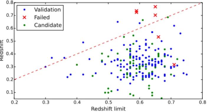
Figure 8. We plot the redshift lower limitzlim(1015)for a cluster with mass
M200=1×10¹⁵M versus cluster photometric redshift for the clusters in the validation sample (blue points) and the clusters we have confirmed in PS1 (green points). Six red crosses mark the systems in the validation sample (with spectroscopic redshifts) that we failed to confirm; we discuss these in Section 4.1. Clusters below the red dashed line have the required PS1 imaging depth to enable a robust redshift measurement. Those clusters above the line are marked as having shallow data in Fig.9.
4.1 Validation using confirmedPlanckclusters
In Fig.8, we plot the redshift lower limitzlim(1015)versus the
mea-sured redshift of the candidates (using spectroscopic redshifts for those previously confirmed clusters). We mark the successful vali-dation clusters in blue, the valivali-dation clusters for which the redshift measurement failed in red, and the new candidates in green. The dashed red line indicates where thezlim(1015)is equal to the cluster
redshift. Candidates that lie below this line have PS1 data that are sufficiently deep given the actual cluster redshift that we expect to extract a robust photo-z. Candidates above the line would bene-fit from deeper imaging data, and for this reason we flag them as ‘shallow’.
Beyond the redshift limit, we can reliably assign a redshift for some candidates, and this is not surprising. The model we adopt in estimating the redshift lower limitzlim(1015)assumes a particular
cluster mass, and manyPlanckcandidates are indeed even more massive. Also, our model does not account for the scatter in the expected number of red galaxies in a cluster at a particular redshift and mass. In general, we would expect the photo-zs for these sys-tems to be less robust, and indeed, we find that these syssys-tems show larger photometric redshift errors than the rest of the candidates.
The blinded photo-zestimation method fails to recover 6 of the 150Planck-confirmed clusters in the validation sample. Four of these cases correspond to clusters with redshifts above 0.7, which are beyond the redshift lower limitszlim(1015) estimated from the
depths of the PS1 data. The other two failures are at redshifts below the estimated redshift lower limit. One of these isPlanck484, which is a low-zcluster which is physically offset from the SZE detection by more than 5 arcmin. In this case, we repeat the analysis after recentring on the correct position and recover thePlanckredshift. The last failure corresponds to the clusterPlanck556 which is at a redshift ofz ≈ 0.71. We note that in this case there is a low significance detection in the likelihood histogram, but we were not able to confirm it as a cluster. A possible explanation is that this system has a somewhat lower mass than the characteristic mass we adopt in estimating the redshift lower limit. Indeed, we find that both of these failed systems have relatively low values ofYSZ,
suggesting that they are lower mass systems. Given the overall success (148/150) of the validation set, we are satisfied that if our depth estimate indicates we should be able to measure a cluster photometric redshift we will be able to do that with good reliability. We also note that Rozo et al. (2014) present a comparison of the
Planckredshifts with the redMaPPer result based on SDSS data. We cross-match the validation sample used here with the 3σ outliers from table 1 of Rozo et al. (2014) and present the result in Table1.
Table 1. Photo-zcomparison for Rozo et al. (2014) sample. ID Planck SDSS PS1 Rozo’s comment
13 0.429 0.325 0.35 97 0.361 0.310 0.29 216 0.336 0.359 0.30 Mismatch 443 0.437 0.221 0.22 484 0.317 – – Unconvincing 500 0.280 0.514 0.32 Bad photometry 527 0.385 – 0.32 Unconvincing 537 0.353 0.287 0.30 865 0.278 0.234 0.24 1216 0.215 – 0.24 redMaPPer incompleteness
Note.The final correct redshift marked by Rozo et al. (2014) is written in bold.
Figure 9. The photo-zmeasurements forPlanckconfirmed clusters plotted versus the spectroscopic redshifts (blue points). The red crosses mark the failures in our photo-zestimation. The black crosses mark the clusters whose redshifts are higher than the redshift limits, and the green squares marks the outliers examined in Rozo et al. (2014).
Our results for the outliers are generally more consistent with the results from Rozo et al. (2014).
After estimating the redshifts for all candidates, we compare the photometric redshifts of the validation clusters with their spectro-scopic redshifts and present this distribution in Fig.9. After re-moving the failures and the questionable clusters identified in Rozo et al. (2014), we are left with 135Planck clusters. We measure the rms scatter defined as (zphoto−zspec)/(1+zspec) using the full
spectroscopic cluster sample to be 0.023. We note that the redshift error distribution has a slight bias (0.003) that can be characterized empirically by a linear model. We apply the bias correction to the measured candidate redshift values when quoting the final photo-z estimation. After applying this bias correction, we obtain an rms value of 0.022. This value compares favourably with that of Song et al. (2012b) who measure an rms scatter for three different pho-tometric redshift estimation methods of between 0.028 and 0.024. We are satisfied that the measured rms in this work demonstrates our ability to measure photometric redshifts for thePlanckcluster candidates with the PS1 data.
Similar to Song et al. (2012b), we estimate the final photo-z uncertainty as the quadrature sum of the measurement uncertainty and an intrinsic or systematic uncertaintyδsys:2zphot=δ2zphot+ δ2
sys. We findδsys=0.007 by requiring that the reducedχ2=1 of
the photometric redshifts about the spectroscopic redshifts for the validation ensemble.
4.2 Results from random sky regions
Random superposition is one source of contamination in our analy-sis. Given the large search radius (5 arcmin), the chance to associate an SZE selected candidate to a lower mass optical system is higher than the in our previous experience with the South Pole Telescope (SPT) sample. Thus, we test our confirmation procedure against randomly selected sky regions to estimate the contamination rate.
We select 60 random candidate positions lying within an large equatorial region we are processing for other purposes; we pro-duce coadds and calibrated cataloguess in the same manner as for the realPlanck candidates. Then we search for optical counter-parts around all random positions, and – where possible – estimate
Table 2. Sky positions and redshifts ofPlanckcandidates.
ID zphot zphot αBCG δBCG zlim(1015)
43 0.077 0.007 253.0509 −0.3377 0.58 59 0.284 0.013 313.5165 −22.8076 0.59 66 0.533 0.250 330.7982 −24.6406 0.55 70 0.284 0.020 257.9357 7.2559 0.62 83 0.425 0.022 344.8704 −25.1154 0.57 111 0.251 0.029 323.2163 −12.5426 0.59 116 0.479 0.037 266.7882 17.1839 0.58 126 0.240 0.021 316.1941 −4.7623 0.56 133 0.229 0.034 273.5555 18.2843 0.57 142 0.360 0.016 219.4179 30.2001 0.72 142∗ 0.170 0.010 219.4585 30.4253 0.72 143 0.240 0.007 252.5850 26.9726 0.70 149 0.544 0.070 335.0728 −12.1916 0.58 150 0.381 0.031 347.4625 −18.3324 0.57 157 0.218 0.046 359.2370 −22.7796 0.56 209 0.403 0.035 313.2155 17.9064 0.48 212 0.403 0.007 257.6559 40.4314 0.66 213 0.686 0.133 229.0082 39.7408 0.69 218 0.273 0.034 319.8591 15.3518 0.54 257 0.436 0.054 242.2561 50.0867 0.68 261 0.088 0.007 290.8001 48.2705 0.57 262 0.479 0.022 3.8511 −17.5108 0.64 282 0.316 0.021 324.4442 35.5975 0.40 289 0.099 0.007 300.8065 51.3474 0.49 305 0.207 0.012 352.1669 7.5801 0.61 314 0.262 0.026 257.4693 62.3689 0.64 375 0.099 0.034 283.0395 72.9927 0.64 383 0.360 0.028 284.2933 74.9421 0.64 420 0.229 0.018 0.3115 50.2756 0.45 509 0.284 0.031 140.0173 70.8205 0.60 522 0.077 0.007 27.8319 10.8141 0.64 529 0.110 0.007 99.4772 66.8518 0.51 543 0.131 0.046 129.9560 62.4101 0.50 553 0.349 0.031 100.1444 57.7460 0.54 554 0.305 0.019 36.2339 8.8299 0.60 554∗ 0.310 0.019 36.1653 8.8983 0.60 575 0.294 0.088 119.3808 52.6829 0.60 576 0.153 0.014 150.4115 50.0149 0.65 612 0.349 0.034 60.7362 9.7414 0.63 618 0.370 0.365 100.7427 31.7503 0.48 679 0.251 0.018 48.8412 −18.2062 0.57 682 0.381 0.036 112.5014 11.9483 0.63 699 0.381 0.086 146.1786 19.4666 0.50 701 0.316 0.045 179.8416 26.4511 0.66 723 0.327 0.027 117.2153 1.1111 0.62 725 0.305 0.028 32.2630 −27.5107 0.58 735 0.131 0.049 78.7192 −19.9555 0.61 736 0.664 0.007 48.7537 −27.3029 0.63 743 0.381 0.066 160.2901 17.5098 0.61 748 0.099 0.007 112.8076 −7.8093 0.68 752 0.294 0.013 120.4230 −4.0614 0.50 778 0.403 0.028 94.7096 −23.5784 0.57 828 0.251 0.044 126.6873 −23.2611 0.53 837 0.436 0.307 131.7742 −21.9784 0.56 860 0.338 0.020 142.9920 −20.6231 0.56 913 0.392 0.067 158.8869 −20.8495 0.57 978 0.327 0.036 175.3720 −21.6974 0.66 1001 0.349 0.025 178.5667 −26.1542 0.57 1080 0.207 0.137 195.4422 −12.0830 0.58 1159 0.055 0.007 201.6415 11.3018 0.64 1178 0.294 0.028 223.1756 −18.5844 0.67 1189 0.305 0.021 216.3013 −4.9427 0.60 1189∗ 0.330 0.021 216.3943 −5.0097 0.68
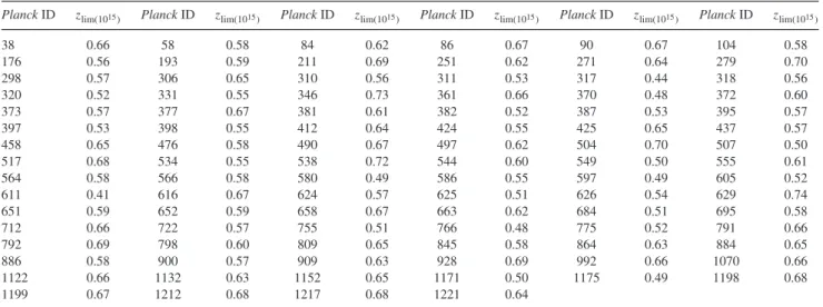
Table 3. UnconfirmedPlanckcluster candidates with redshift lower limitszlim(1015).
PlanckID zlim(1015) PlanckID zlim(1015) PlanckID zlim(1015) PlanckID zlim(1015) PlanckID zlim(1015) PlanckID zlim(1015)
38 0.66 58 0.58 84 0.62 86 0.67 90 0.67 104 0.58 176 0.56 193 0.59 211 0.69 251 0.62 271 0.64 279 0.70 298 0.57 306 0.65 310 0.56 311 0.53 317 0.44 318 0.56 320 0.52 331 0.55 346 0.73 361 0.66 370 0.48 372 0.60 373 0.57 377 0.67 381 0.61 382 0.52 387 0.53 395 0.57 397 0.53 398 0.55 412 0.64 424 0.55 425 0.65 437 0.57 458 0.65 476 0.58 490 0.67 497 0.62 504 0.70 507 0.50 517 0.68 534 0.55 538 0.72 544 0.60 549 0.50 555 0.61 564 0.58 566 0.58 580 0.49 586 0.55 597 0.49 605 0.52 611 0.41 616 0.67 624 0.57 625 0.51 626 0.54 629 0.74 651 0.59 652 0.59 658 0.67 663 0.62 684 0.51 695 0.58 712 0.66 722 0.57 755 0.51 766 0.48 775 0.52 791 0.66 792 0.69 798 0.60 809 0.65 845 0.58 864 0.63 884 0.65 886 0.58 900 0.57 909 0.63 928 0.69 992 0.66 1070 0.66 1122 0.66 1132 0.63 1152 0.65 1171 0.50 1175 0.49 1198 0.68 1199 0.67 1212 0.68 1217 0.68 1221 0.64
redshifts. Out of the 60 random positions, we identify six candidates that exhibit weak significance in their likelihood distributions and pass our detection threshold. Further, two of these pass the second round visual examination where we require a clustered collection of galaxies. Using SIMBAD, we find that one of them is a known cluster identified by De Propris et al. (2002) in the 2dF survey, but the other candidate is not associated with any previously known cluster (Wenger et al.2000). The results of this test indicate that our method applied toPlanckcandidates and PS1 data suffers from a contamination rate of approximately∼3 per cent.
4.3 Results from thePlanckcandidates sample
We are able to identify optical counterparts and measure redshifts for 60 of the full sample of 237 Planckcandidates. The Planck
ID, the BCG sky position (αBCG,δBCG), the photometric redshift
measurement and the redshift lower limit zlim(1015) are presented
in Table 2. An additional 83 candidates are located so close to the Galactic plane (see Fig. 1) that we cannot reliably assign a redshift or a redshift lower limit due to the high stellar density. For the remaining 94 candidates, we are unable to identify an optical counterpart and we provide only redshift lower limitszlim(1015)that
reflect the depths of the catalogue at those candidate locations. This information together with thePlanckID is presented for each candidate in Table3.
19 of the confirmed candidates are in Planck Class 1 (cf. Section 2.1 for thePlanckclassification), whereas there are only three Class 1 candidates remaining in the 94 candidates. This shows that our algorithm has confirmed most of the reliable detections from thePlanckcatalogue. And the three remaining candidates may re-side at redshifts beyond our redshift limits where deeper imaging is needed.
Using contamination estimates from the Planck Collaboration XXIX (2014a) together with the number of totalPlanckcandidates and previously confirmed clusters, we estimate that only 45 per cent of our sample (∼110) should be real clusters. If we take our confirmed sample of 60 clusters together with 45 per cent of the 83 candidates lying in fields with high stellar contamination, we have accounted for 98 of our estimates 110 expected real clusters. Thus, these numbers suggest that as many as 12 of our 94 unconfirmed candidates would likely turn out to be real clusters lying at redshifts beyond the redshift lower limitszlim(1015)we present.
Note that because the contamination rate is higher in thePlanck
catalogue in regions of high Galactic dust Planck Collaboration XXIX (2014a), the number of potentially unconfirmed clusters in the 83 candidates close to the Galactic plane may be less than our estimate. This introduces additional uncertainty into our esti-mate of the expected number of unconfirmed candidates lying at
z > zlim(1015).
Recently, Planck Collaboration XXVI (2014b) published newly confirmed clusters using data from the Russian–Turkish 1.5 m tele-scope and 6 m Bolshoy Teletele-scope Azimutal’ny of the Special Astrophysical Observatory of the Russian Academy of Sciences. They confirmed 41 newPlanckSZE clusters. We cross-match our sample with their results, finding that 11 clusters are in a good agreement and two others (candidates 383 and 618) exhibit large discrepancies (z >0.1). In both of these cases, our results prefer lower redshifts. For the remaining 28 confirmed systems, we mark 16 as lying in star fields, and the rest are not fully covered in the PS1 data.
5 C O N C L U S I O N S
We study 237 unconfirmedPlanckcluster candidates that overlap the PS1 footprint. We describe the production of science ready catalogues and present the distribution of measured depths and photometric quality for this ensemble of cluster candidates. We summarize our method for estimating cluster photometric redshifts and describe a method for estimating a redshift lower limitzlim(1015)
beyond which we would not expect to be able to have confirmed the cluster in the PS1 data. This method uses what we know about SZE selected massive clusters from SPT together with the measured depths of the PS1 catalogues.
We validate our photometric redshift estimation with a sample of 150Planckconfirmed clusters. In this test, we fail to detect four clusters that are beyond the redshift limit of the PS1 data, and two clusters that are within the redshift limits given the PS1 data quality. We find that 6 out of 10 previously identified clusters exhibiting large redshift discrepancies when comparing thePlanckand Rozo et al. (2014) results exhibit redshifts that are more consistent with the Rozo et al. (2014) result. For the remaining clusters, we achieve an overall redshift scatter of (zphoto−zspec)/(1+zspec)∼0.022. We
also examine the false detection rate due to random superposition of low-mass galaxy systems. Using 60 random sky regions, we find
a contamination rate of∼3 per cent, indicating that this fraction of our confirmed sample may be contaminated.
Using these data products and methods, we measure photometric redshifts for 60Planckcandidates. The newly confirmed clusters span a redshift range 0.06< z <0.69 with a median redshiftzmed=
0.31, which is consistent with the redshift distribution presented for the previously confirmed sample ofPlanckselected clusters. This sample of 60 newly confirmed clusters increases the total number of new,Planckdiscovered clusters from 178 to 238, bringing the totalPlanckcluster sample – including those discovered in previous surveys – to 921 (Planck Collaboration XXIX2014a).
We exclude 83 of the remaining candidates because of high stellar contamination due to their position close to the Galactic plane. For these systems we cannot obtain reliable photometric redshifts or estimate redshift lower limits with the current data. We are unable to find optical counterparts or estimate photometric redshifts for the last 94 candidates in our sample. For each of these we present a redshift lower limitzlim(1015), but the majority of these systems are
expected to be noise fluctuations.
Using contamination estimates from the Planck Collaboration XXIX (2014a), we estimate that∼12 of the 94 unconfirmed can-didates could turn out to be real clusters lying at redshifts beyond the redshift lower limitszlim(1015)we present. Confirming these
sys-tems will require short exposures on 4-m or 6.5-m class telescopes. AdditionalPlanckcandidates can be obtained by mining the newly available DES data in the southern celestial hemisphere. The DES depths are adequate to identify the optical counterparts and mea-sure redshifts for high-mass clusters out toz∼1.2 (Hennig et al., in preparation).
AC K N OW L E D G E M E N T S
The Munich group at LMU is supported by the DFG through TR33 ‘The Dark Universe’ and the Cluster of Excellence ‘Origin and Structure of the Universe’. The data processing has been carried out on the computing facilities of the Computational Center for Particle and Astrophysics (C2PAP), which is supported by the Cluster of Excellence. We want to thank H. H. Head from Austin Peay state university, with whom we initiated this project. Also we would like to thank J. Dietrich and D. C. Gangkofner at LMU for helpful discussions.
The Pan-STARRS1 Surveys (PS1) have been made possible through contributions of the Institute for Astronomy, the Univer-sity of Hawaii, the Pan-STARRS Project Office, the Max-Planck Society and its participating institutes, the Max Planck Institute for Astronomy, Heidelberg and the Max Planck Institute for Extrater-restrial Physics, Garching, The Johns Hopkins University, Durham University, the University of Edinburgh, Queen’s University Belfast, the Harvard–Smithsonian Center for Astrophysics, the Las Cumbres Observatory Global Telescope Network Incorporated, the National Central University of Taiwan, the Space Telescope Science Institute, the National Aeronautics and Space Administration under grant no. NNX08AR22G issued through the Planetary Science Division of the NASA Science Mission Directorate, the National Science Foun-dation under grant no. AST-1238877, the University of Maryland and Eotvos Lorand University (ELTE).
R E F E R E N C E S
Abell G. O., 1958, ApJS, 3, 211
Abell G. O., Corwin H. G., Jr, Olowin R. P., 1989, ApJS, 70, 1
Bertin E., 2011, in Evans I. N., Accomazzi A., Mink D. J., Rots A. H., eds, ASP Conf. Ser. Vol. 442, Astronomical Data Analysis Software and Systems XX. Astron. Soc. Pac., San Francisco, p. 435
Bertin E., Arnouts S., 1996, A&AS, 117, 393
Bertin E., Mellier Y., Radovich M., Missonnier G., Didelon P., Morin B., 2002, in Bohlender D. A., Durand D., Handley T. H., eds, ASP Conf. Ser. Vol. 281, Astronomical Data Analysis Software and Systems XI. Astron. Soc. Pac., San Francisco, p. 228
Bleem L. E. et al., 2015, ApJS, 216, 27 Bocquet S. et al., 2015, ApJ, 799, 214 B¨ohringer H. et al., 2004, A&A, 425, 367
Bouy H., Bertin E., Moraux E., Cuillandre J.-C., Bouvier J., Barrado D., Solano E., Bayo A., 2013, A&A, 554, A101
Bruzual G., Charlot S., 2003, MNRAS, 344, 1000
Carvalho P., Rocha G., Hobson M. P., Lasenby A., 2012, MNRAS, 427, 1384
De Propris R. et al., 2002, MNRAS, 329, 87 Desai S. et al., 2012, ApJ, 757, 83
Duffy A. R., Schaye J., Kay S. T., Dalla Vecchia C., 2008, MNRAS, 390, L64
Eke V. R., Cole S., Frenk C. S., 1996, MNRAS, 282, 263 Gladders M. D., Yee H. K. C., 2005, ApJS, 157, 1 Hao J. et al., 2010, ApJS, 191, 254
Hasselfield M. et al., 2013, J. Cosmol. Astropart. Phys., 7, 8
High F. W., Stubbs C. W., Rest A., Stalder B., Challis P., 2009, AJ, 138, 110
Hoyle B., Jimenez R., Verde L., Hotchkiss S., 2012, J. Cosmol. Astropart. Phys., 2, 9
Kaiser N. et al., 2002, in Tyson J. A., Wolff S., eds, Proc. SPIE Conf. Ser. Vol. 4836, Survey and Other Telescope Technologies and Discoveries. SPIE, Bellingham, p. 154
Klein J. R., Roodman A., 2005, Ann. Rev. Nucl. Part. Sci., 55, 141 Koester B. P. et al., 2007, ApJ, 660, 239
Lin Y., Mohr J. J., Stanford S. A., 2004, ApJ, 610, 745
Mana A., Giannantonio T., Weller J., Hoyle B., H¨utsi G., Sartoris B., 2013, MNRAS, 434, 684
Mancone C. L., Gonzalez A. H., 2012, PASP, 124, 606
Mantz A., Allen S. W., Rapetti D., Ebeling H., 2010, MNRAS, 406, 1759 Mehrtens N. et al., 2012, MNRAS, 423, 1024
Melin J.-B., Bartlett J. G., Delabrouille J., 2006, A&A, 459, 341 Melin J.-B. et al., 2012, A&A, 548, A51
Metcalfe N. et al., 2013, MNRAS, 435, 1825
Mohr J. J. et al., 2008, in Brissenden R. J., Silva D. R., eds, Proc. SPIE Conf. Ser. Vol. 7016, Observatory Operations: Strategies, Processes, and Systems II. SPIE, Bellingham, p. 70160L
Mohr J. J. et al., 2012, in Radziwill N. M., Chiozzieds G., Proc. SPIE Conf. Ser. Vol. 8451, Software and Cyberinfrastructure for Astronomy II. SPIE, Bellingham, p. 84510D
Navarro J. F., Frenk C. S., White S. D. M., 1997, ApJ, 490, 493
Ngeow C. et al., 2006, in Silva D. R., Doxsey R. E., eds, Proc. SPIE Conf. Ser. Vol. 6270, Observatory Operations: Strategies, Processes, and Systems. SPIE, Bellingham, p. 627023
Piffaretti R., Arnaud M., Pratt G. W., Pointecouteau E., Melin J.-B., 2011, A&A, 534, A109
Planck Collaboration XXIX, 2014a, A&A, 571, A29
Planck Collaboration XXVI, 2014b, preprint (arXiv:1407.6663) Poggianti B. M. et al., 2001, ApJ, 562, 689
Reichardt C. L. et al., 2013, ApJ, 763, 127
Rosati P., della Ceca R., Norman C., Giacconi R., 1998, ApJ, 492, L21 Rozo E. et al., 2010, ApJ, 708, 645
Rozo E., Rykoff E. S., Bartlett J. G., Melin J. B., 2014, preprint (arXiv:1401.7716)
Schechter P., 1976, ApJ, 203, 297 Schlafly E. F. et al., 2012, ApJ, 756, 158
Schlegel D. J., Finkbeiner D. P., Davis M., 1998, ApJ, 500, 525 Skrutskie M. F. et al., 2006, AJ, 131, 1163
Song J., Mohr J. J., Barkhouse W. A., Warren M. S., Rude C., 2012a, ApJ, 747, 58
Song J. et al., 2012b, ApJ, 761, 22 Staniszewski Z. et al., 2009, ApJ, 701, 32
Sunyaev R. A., Zel’dovich Y. B., 1970, Comments Astrophys. Space Phys., 2, 66
Sunyaev R. A., Zel’dovich Y. B., 1972, Comments Astrophys Space Phys, 4, 173
Szabo T., Pierpaoli E., Dong F., Pipino A., Gunn J., 2011, ApJ, 736, 21 Szalay A. S., Connolly A. J., Szokoly G. P., 1999, AJ, 117, 68 Tonry J. L. et al., 2012, ApJ, 750, 99
Vikhlinin A. et al., 2009, ApJ, 692, 1060
Voges W. et al., 1999, A&A, 349, 389
Wen Z. L., Han J. L., Liu F. S., 2012, ApJS, 199, 34 Wenger M. et al., 2000, A&AS, 143, 9
White S. D. M., Efstathiou G., Frenk C. S., 1993, MNRAS, 262, 1023 Williamson R. et al., 2011, ApJ, 738, 139
Wright E. L. et al., 2010, AJ, 140, 1868 York D. G. et al., 2000, AJ, 120, 1579