Le
´vy(-Type) Processes
Von der
Fakult¨at Mathematik und Naturwissenschaften Technische Universit¨at Dresden
genehmigte
Dissertation
zur Erlangung des akademischen Grades
Doctor rerum naturalium
(Dr. rer. nat.)
vonDipl.-Math. Franziska K¨
uhn
geboren am 01. November 1989 in DresdenDie Dissertation wurde in der Zeit von Juni 2014 bis Juli 2016 unter der Betreuung von Prof. Dr. Rene´ L. Schilling im Institut f¨ur Mathematische Stochastik angefertigt.
Eingereicht am 12. Juli 2016 Tag der Disputation: 25. November 2016 Gutachter: Prof. Dr. Rene´ L. Schilling, TU Dresden
Index of notation iii
Summary 1
1 Basics 7
1.1 Probability theory & stochastic processes . . . 9
1.2 Markov processes . . . 10 1.3 Le´vy processes . . . 13 1.4 Subordination . . . 16 1.5 Feller processes . . . 17 1.6 Martingale problem . . . 25 1.7 Parametrix method . . . 30
2 Moments of Le´vy-type processes 35 2.1 Existence of moments . . . 35
2.2 Fractional moments . . . 41
2.3 Absolute continuity of Le´vy-type processes with H¨older continuous symbols 44 3 Parametrix construction 51 3.1 Main results . . . 53
3.2 Extensions . . . 59
3.3 Open problems . . . 61
4 Parametrix construction: proofs 63 4.1 Heat kernel estimates for rotationally invariant Le´vy processes . . . 65
4.2 Auxiliary convolution estimates . . . 81
4.3 A candidate for the transition density . . . 91
4.4 Time derivative . . . 98
4.5 Strong continuity of the prospective semigroup . . . 103
4.6 The approximating fundamental solution . . . 109
4.7 (𝑃𝑡)𝑡≥0 as a Markov semigroup . . . 125
4.8 Proof of the main results . . . 129
4.9 Proof of Theorem 3.7, Theorem 3.8 and Corollary 3.9 . . . 131
5 Applications 143
5.1 Variable order subordination . . . 143
5.2 Feller processes with symbols of varying order . . . 166
5.3 Mixing . . . 169
5.4 Solutions of Le´vy-driven SDEs with H¨older continuous coefficients . . . 174
A Appendix 181 A.1 Slowly varying functions . . . 181
A.2 Auxiliary results . . . 183
Analysis
inf∅ inf∅ = +∞
𝑥⊺,𝐴⊺ transpose
𝑥⋅𝑦 Euclidean scalar product
𝑎∨𝑏, 𝑎∧𝑏 maximum, minimum arg𝑧 ∈ (−𝜋, 𝜋⌋︀, argument of𝑧∈ℂ
tr𝐴 trace of the matrix𝐴
♯𝐴 cardinality of the set𝐴
1𝐴 indicator function of the set𝐴
spt𝑓 support of𝑓
∇𝑓 gradient ∇2𝑓 Hessian matrix
𝑓(𝑡−) left limit lim𝑠↑𝑡𝑓(𝑠) ca`dla`g finite left limits and
right-continuous ca`gla`d finite right limits and
left-continuous ∏︁ ⋅ ∏︁∞ uniform norm ∏︁ ⋅ ∏︁(2) norm on𝐶 2 𝑏(ℝ 𝑑), p. 7 Γ Gamma function (𝑧)𝛼 =Γ(𝑧+𝛼)⇑Γ(𝑧), Pochhammer symbol
Log complex logarithm (principal value)
arctan arctangent
𝑓+, 𝑓− positive part, negative part
𝑓∗𝑔 convolution 𝑓⊛𝑔 time-space convolution, p. 8 𝑓○𝑔 composition ^ 𝑓,F𝑓 Fourier transform ˇ
𝑓,F−1𝑓 inverse Fourier transform
(𝐴,D) closure of operator𝐴∶D→𝐴(D) Probability/measure theory á stochastic independence ∼ distributed as 𝑑 = equality in distribution 𝑣 → vague convergence 𝑤 → weak convergence B(ℝ𝑑) Borel𝜎-algebra onℝ𝑑 A⊗B product𝜎-algebra 𝛿𝑥 Dirac measure at𝑥
ℙ 𝔼ℙ probability, expectation with respect to ℙ(𝔼=𝔼ℙ for short)
𝔼(⋅ ⋃︀F) conditional expectation with
respect to a𝜎-algebraF
ℙ𝑋 ℙ(𝑋∈ ⋅), distribution of a random
variable𝑋
F𝑡 filtration
F𝑋
𝑡 canonical filtration of stoch. process(𝑋𝑡)𝑡≥0
a.s. almost surely (with respect toℙ)
Spaces of functions
B𝑏(ℝ𝑑) Borel measurable, bounded
functions𝑓 ∶ℝ𝑑→ℝ 𝐶(ℝ𝑑) continuous functions𝑓 ∶ ℝ𝑑→ℝ 𝐶𝑐(ℝ𝑑) —, compact support 𝐶𝑏(ℝ𝑑) —, bounded 𝐶∞(ℝ 𝑑) —, vanishing at infinity lim⋃︀𝑥⋃︀→∞⋃︀𝑓(𝑥)⋃︀ =0
𝐶𝑛(ℝ𝑑) 𝑛-times continuously differentiable
functions
𝐶𝑛 𝑏(ℝ
𝑑) —, bounded (with all derivatives)
𝐶∞𝑛(ℝ
𝑑) —, vanishing at infinity (with all derivatives)
𝐶∞
𝑐 (ℝ𝑑) smooth functions𝑓 ∶ℝ𝑑→ℝwith compact support
𝐶>0(𝐼) p. 160
Sets
𝐴𝑐 complement of the set𝐴 𝐴⋅∪𝐵 disjoint union of𝐴and𝐵 𝐴 closure of the set𝐴
𝐵(𝑥, 𝑟) open ball, centre𝑥, radius𝑟 𝐵(︀𝑥, 𝑟⌋︀ closed ball, centre𝑥, radius𝑟 Markov processes (𝑃𝑡)𝑡≥0 semigroup (𝐿,D(𝐿)) generator 𝑅𝜆 = (𝜆−𝐿)−1, resolvent References (B1)-(B4) p. 144 (C1)-(C4) p. 53 (C5) p. 57 (C6) p. 176 (C3’),(C4’) p. 59 (C4”) p. 168 (C5”) p. 169 (D1),(D2) p. 45 (E1)-(E3) p. 74
(PMP) positive maximum principle, p. 11
Abbreviations
NIG normal inverse Gaussian NTS normal tempered stable TLP truncated Le´vy process
Further notation
𝐴(𝑚) admissible cts. neg. def. fcts., p. 53 Ω(𝑚, 𝜗) p. 53 Λ(𝑚, 𝑅, 𝜗) p. 144 𝐶(𝜗) p. 144 𝑆(𝑥, 𝛼, 𝑡) p. 56 𝐹(𝑡, 𝑥, 𝑦) p. 64 𝐺(𝑡, 𝑥, 𝑦) p. 94 𝐻𝑘(𝑡, 𝑥, 𝑦) p. 95 Φ(𝑡, 𝑥, 𝑦) p. 97 𝑔𝛾(𝑥) p. 81 𝑝𝛼𝑡(𝑥) p. 63 𝑝0(𝑡, 𝑥, 𝑦) parametrix, p. 63
𝑝𝜀(𝑡, 𝑥, 𝑦) approximate fundamental solution, p. 110
𝐴𝛽𝑝𝛼
𝑡 p. 63
Le´vy processes are stochastic processes with independent and stationary increments. They constitute an important subclass of Markov processes. By the Le´vy-Khintchine formula, there is a one-to-one correspondence between Le´vy processes and continuous negative definite (in the sense of Schoenberg [8]) functions. In particular, any Le´vy process can be uniquely determined by a continuous negative definite function𝜓, the so-called characteristic exponent, 𝜓(𝜉) = −𝑖𝑏⋅𝜉+1 2𝜉⋅𝑄𝜉+ ∫ℝ𝑑/{0}( 1−𝑒𝑖𝑦⋅𝜉+ 𝑖𝑦⋅𝜉1(0,1)(⋃︀𝑦⋃︀))𝜈(𝑑𝑦), 𝜉∈ℝ 𝑑,
where(𝑏, 𝑄, 𝜈)is the Le´vy triplet comprising the drift𝑏∈ℝ𝑑, the diffusion matrix 𝑄∈ℝ𝑑×𝑑, and the Le´vy measure𝜈. Many distributional properties and path properties of a Le´vy process can be described in terms of the characteristic exponent 𝜓 or the Le´vy triplet, see e. g. Sato [92, Chapter 4,5], Blumenthal & Getoor [12] and Fristedt [38].
There are other, larger subclasses of Markov processes which can be characterized in terms of a single deterministic function. In this thesis, we focus on, so-called, Feller processes. Roughly speaking, Feller processes behave locally like Le´vy processes – that’s the reason why they are also called Le´vy-type processes – but, in contrast to Le´vy processes, Feller processes need not to be homogeneous in space. Typical examples of Feller processes are solutions of Le´vy-driven stochastic differential equations (SDEs, for short), affine processes and stable-like processes.
If a Feller process has the additional property that the smooth functions with compact support are contained in the domain of the generator, then we speak of a rich Feller process. Any such rich Feller process can be characterized by its𝑥-dependent symbol
𝑞(𝑥, 𝜉) = −𝑖𝑏(𝑥) ⋅𝜉+1
2𝜉⋅𝑄(𝑥)𝜉+ ∫ℝ𝑑/{0}(
1−𝑒𝑖𝑦⋅𝜉+
𝑖𝑦⋅𝜉1(0,1)(⋃︀𝑦⋃︀))𝜈(𝑥, 𝑑𝑦), 𝑥, 𝜉∈ℝ
𝑑
which is the analogue of the characteristic exponent in the Le´vy case. Restricted to the smooth functions with compact support, the generator of a rich Feller process is a pseudo-differential operator with symbol 𝑞. Among the first to study the connection between rich Feller processes and pseudo-differential operators with negative definite symbols was Jacob [49, 50, 51].
Since Feller processes behave locally like Le´vy processes, it is a natural guess that the symbol plays a similar role as the characteristic exponent in the theory of Le´vy processes, i. e. that it is a useful tool to describe properties of the process. This has been confirmed by many authors who studied properties of Feller processes in the past years, such as recurrence & transience (Sandric [89]), ergodicity (Sandric [90]), invariant measures (Behme & Schnurr [6]), Hausdorff dimensions (see [19, Section 5.2] and the references therein), the asymptotic growth of the sample paths (Schilling [94], Knopova & Schilling [58]) and Besov regularity ([19, Section 5.5]).
In the first part of this thesis, Chapter 2, we will investigate a distributional property of Feller processes which has barely received any attention so far: existence of generalized moments and moment estimates. For a Le´vy process (𝐿𝑡)𝑡≥0 and a locally bounded submultiplicative function𝑓 ∶ℝ𝑑→ (︀0,∞), it is well-known (cf. Sato [92]) that the existence of the generalized moment𝔼𝑥𝑓(𝐿𝑡) can equivalently be characterized in terms of the Le´vy
measure 𝜈:
𝔼𝑥𝑓(𝐿𝑡) < ∞ ⇐⇒ ∫
⋃︀𝑦⋃︀≥1
𝑓(𝑦)𝜈(𝑑𝑦) < ∞.
This implies, in particular, that the existence of generalized moments is a time-independent distributional property, i. e.
∃𝑡>0∶𝔼𝑥𝑓(𝐿𝑡) < ∞ ⇐⇒ ∀𝑡>0∶𝔼𝑥𝑓(𝐿𝑡) < ∞.
In Section 2.1 we will establish similar results for Feller processes. We will show that generalized moments exist backward in time, i. e.
𝔼𝑥𝑓(𝑋𝑡) < ∞ Ô⇒ ∀𝑠≤𝑡∶𝔼𝑥𝑓(𝑋𝑠) < ∞,
and that the moments also exist forward in time provided that𝔼𝑥𝑓(𝑋𝑡−𝑥) is bounded in
𝑥∈ℝ𝑑. Furthermore, Theorem 2.4 will give a sufficient condition for the existence of the moment𝔼𝑥𝑓(𝑋𝑡) in terms of the𝑥-dependent Le´vy triplet(𝑏(𝑥), 𝑄(𝑥), 𝜈(𝑥,⋅)): If 𝑓 ≥0 is comparable to a submultiplicative function 𝑔≥0 which is twice differentiable, then
sup 𝑥∈𝐾∫⋃︀𝑦⋃︀≥1 𝑓(𝑦)𝜈(𝑥, 𝑑𝑦) < ∞ Ô⇒ sup 𝑥∈𝐾 sup 𝑠≤𝑡 𝔼𝑥𝑓(𝑋𝑠∧𝜏𝐾 −𝑥) < ∞
for any compact set 𝐾⊆ℝ𝑑where 𝜏𝐾∶=inf{𝑡≥0;𝑋𝑡∉𝐾}denotes the exit time from the set𝐾; if the symbol 𝑞 of the Feller process (𝑋𝑡)𝑡≥0 has bounded coefficients, then𝐾 =ℝ
𝑑
is admissible.
In applications it is often useful to have moment estimates, and in the last years there has been a particular interest in estimates of fractional moments𝔼⋃︀𝑋𝑡⋃︀𝛼, e. g. to obtain Harnack
inequalities (Deng & Schilling [31]) or to prove the absolute continuity of solutions of Le´vy driven SDEs (Fournier & Printems [36]). In our recent publication [67] we have applied different techniques to establish estimates for fractional moments of Feller processes and succeeded in generalizing results for Le´vy processes obtained by Luschgy & Page`s [72] and Deng & Schilling [31]. Here, in this thesis, we will first introduce the notion of generalized Blumenthal–Getoor indices (following Schilling [94]) and then derive estimates for fractional moments by combining a maximal inequality for Feller processes (Lemma 1.29) with the identity
𝔼(⋃︀𝑋⋃︀𝛾) = ∫
(0,∞)
ℙ(⋃︀𝑋⋃︀ ≥𝑟1⇑𝛾)𝑑𝑟, 𝛾 >0.
This is one of the approaches which we have investigated in [67]. There is also the possibility to prove estimates of fractional moments using the Burkholder–Davis–Gundy inequality; we refer to [67] for details.
Finally, as an application of the moment estimates, we will show the absolute continuity of a class of Feller processes with H¨older continuous symbols (Section 2.3).
From Chapter 3 on we will be concerned with questions on the existence of Feller processes. The Le´vy–Khintchine formula states that for any continuous negative definite function 𝜓
there is a Le´vy process with characteristic exponent 𝜓. This, however, is no longer true for Feller processes: Given an arbitrary family (𝑞(𝑥,⋅))𝑥∈ℝ𝑑 of continuous negative definite functions there does, in general, not exist a Feller process with symbol 𝑞 (see [19, Example 2.26] for counterexamples). For this reason it is crucial to find sufficient conditions on 𝑞 or the associated family of triplets (𝑏(𝑥), 𝑄(𝑥), 𝜈(𝑥,⋅))𝑥∈ℝ𝑑 which ensure the existence of a Feller process with given symbol 𝑞.
There are different techniques to prove existence results for Feller processes, they range from purely analytic approaches (e. g. via the Hille–Yoshida theorem or a parametrix construction) to probabilistic methods (e. g. Feller processes as solutions of martingale problems or solutions of SDEs). We refer to the monograph [19] for a survey on known results.
Our method of choice is the parametrix construction. Its idea goes back to Levi [70] who obtained the fundamental solution of a parabolic differential equation using a parametrix construction. Feller [34] was one of the first to recognize the possible applications in probability theory. Already in 1936 he showed existence results for diffusions processes and a class of jump processes. Over the last two decades, the parametrix method has become an increasingly popular tool to prove the existence of certain stochastic processes and derive heat kernel estimates, e. g. processes with variable order of differentiation (Kolokoltsov [59, 60] and Chen & Zhang [25]), gradient perturbations of Le´vy generators (Bogdan & Jakubowski [13] and Jakubowski & Szczypkowski [55]) and solutions of SDEs with H¨older continuous coefficients (Knopova & Kulik [57] and Huang [45]). Hoh [43] developed a symbolic calculus for pseudo-differential operators with continuous negative definite symbols and used a parametrix construction to obtain rather general existence results for Feller processes. The drawback of his approach is that it requires smoothness of𝑞(⋅, 𝜉). Roughly speaking, there is usually a trade-off between assumptions on the regularity of
𝑥 ↦𝑞(𝑥, 𝜉) and assumptions on 𝜉 ↦ 𝑞(𝑥, 𝜉). If 𝑞(𝑥,⋅) is assumed to be of a particular form (typically “stable-like”), then the existence of a Feller process with symbol 𝑞 can be proved under weak regularity assumptions with respect to the space variable𝑥. In contrast, existence results which are applicable for a broad class of negative definite functions 𝑞(𝑥,⋅)
often require smoothness of the symbol with respect to 𝑥.
Since we are interested in existence results under weak regularity of 𝑞(⋅, 𝜉), we have to make some assumptions on the structure of 𝑞. We will consider families of continuous negative definite functions (𝑞(𝑥,⋅))𝑥∈ℝ𝑑 which can be written in the form
𝑞(𝑥, 𝜉) =𝜓𝛼(𝑥)(𝜉), 𝑥, 𝜉∈ℝ
𝑑,
for a H¨older continuous mapping 𝛼 ∶ℝ𝑑 →𝐼 ⊆ ℝ𝑛 and a family 𝜓𝛽 ∶ℝ𝑑 →ℂ, 𝛽 ∈ 𝐼, of continuous negative definite functions. Our main result, Theorem 3.2, states that if
• 𝜓𝛽 is rotationally invariant, i. e. there exists a mapping Ψ𝛽 ∶ ℝ → ℝ such that
• 𝐼 ∋𝛽 ↦Ψ𝛽(𝜉) admits partial derivatives and both Ψ𝛽 and the partial derivatives 𝜕𝛽𝑗Ψ𝛽,𝑗=1, . . . , 𝑛, have a holomorphic extension to a certain domain Ω⊆ℂ,
• Ψ𝛽 and 𝜕𝛽𝑗Ψ𝛽 satisfy certain growth conditions on Ω, then there exists a Feller process (𝑋𝑡)𝑡≥0 with symbol
𝑞(𝑥, 𝜉) ∶=𝜓𝛼(𝑥)(𝜉), 𝑥, 𝜉∈ℝ
𝑑.
In dimension𝑑=1 we can drop the assumption of rotational invariance (Theorem 3.7). As a by-product of the parametrix construction, we get additional information on the Feller process(𝑋𝑡)𝑡≥0:
• The smooth functions with compact support𝐶∞
𝑐 (ℝ𝑑) are a core for the generator𝐿
of the Feller process(𝑋𝑡)𝑡≥0 (Proposition 3.3).
• The(𝐿, 𝐶∞
𝑐 (ℝ𝑑))-martingale problem is well-posed and its unique solution is given
by(𝑋𝑡)𝑡≥0 (Corollary 3.5).
• The transition probability ℙ𝑥(𝑋𝑡∈ ⋅),𝑡>0, has a density𝑝=𝑝(𝑡, 𝑥, 𝑦) with respect
to Lebesgue measure (Theorem 3.2). The density𝑝 is the fundamental solution to the Cauchy problem for the operator𝜕𝑡−𝐿(Corollary 3.4).
• We obtain heat kernel estimates for the transition density𝑝 and its time derivative (Theorem 3.6). In dimension𝑑=1 we also get heat kernel estimates for the derivative with respect to𝑥 (Theorem 3.8).
• In dimension𝑑=1, the Feller process(𝑋𝑡)𝑡≥0 is irreducible with respect to Lebesgue measure if 𝛼∈𝐶𝑏2(ℝ) (Corollary 3.9).
We will prove these results in Chapter 4 using a parametrix construction. The proof has been inspired by the works of Kolokoltsov [60] and Knopova & Kulik [57]. In the first part of the proof, Section 4.1, we will derive heat kernel estimates for a class of rotationally invariant Le´vy processes which, we believe, are of independent interest.
Chapter 5 is devoted to applications of the existence result. Because of the assumption of rotational invariance in dimension 𝑑>1, it is natural to consider symbols which can be expressed in the form
𝑞(𝑥, 𝜉) =𝑓𝛼(𝑥)(⋃︀𝜉⋃︀
2), 𝑥, 𝜉∈
ℝ𝑑,
for a family of Bernstein functions(𝑓𝛽)𝛽∈𝐼 and a H¨older continuous mapping 𝛼∶ℝ
𝑑→𝐼.
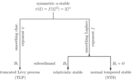
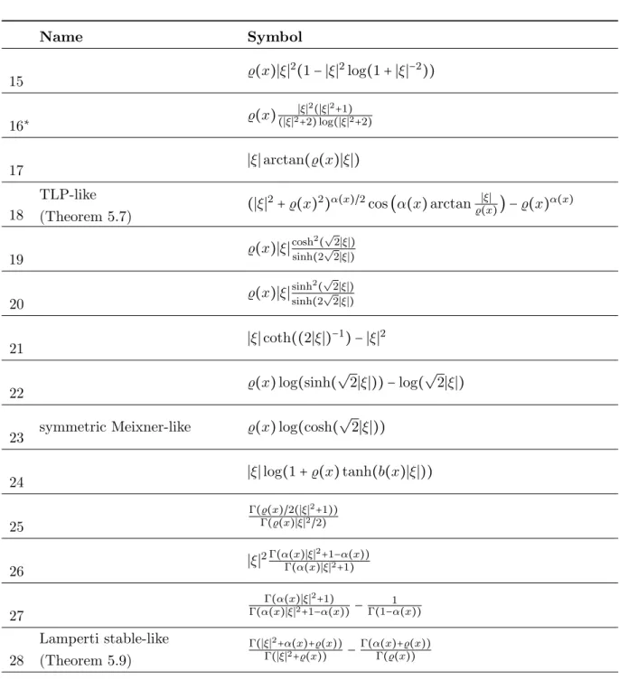
This is a particular case of, so-called, variable order subordination. In Section 5.1 we will present examples of Bernstein functions which satisfy the assumptions of our existence theorem. We will establish, among others, the existence of relativistic stable-like, Lamperti stable-like and normal tempered stable-like Feller processes. Further examples are collected in Table 5.1. Compared to other results in the literature (e. g. Hoh [43]), the novelty is
that𝛼 need not to be smooth; it suffices to have H¨older continuity. Section 5.2 deals with Feller processes with symbols of varying order,
𝑞(𝑥, 𝜉) = (𝑝(𝑥, 𝜉))𝛼(𝑥)
, 𝑥, 𝜉∈ℝ𝑑,
and in Section 5.3 we will obtain existence results for Feller processes of a mixed type. Finally, in the last part of Chapter 5, we will investigate Le´vy-driven SDEs with H¨older continuous coefficients 𝑏 and𝜎,
𝑑𝑋𝑡=𝑏(𝑋𝑡−)𝑑𝑡+𝜎(𝑋𝑡−)𝑑𝐿𝑡.
For a certain class of driving Le´vy processes(𝐿𝑡)𝑡≥0 we will show the existence of a unique weak solution to the SDE and that the solution is a Feller process (Corollary 5.19). This result was previously known only for isotropic 𝛼-stable Le´vy processes (see Knopova & Kulik [57] and the references therein).
Further research – not related to the topics presented in this thesis – can be found in the joint work [69] with Rene´ Schilling which appeared inJournal of Theoretical Probability
recently. It is concerned with moderate deviation principles for additive processes and resulted from my diploma thesis [66].
It is my pleasure to thank the many people who have, the one way or the other, contributed to this thesis. My thanks goes to all friends and colleagues who supported me in the past two years, whether it was by providing welcome distraction from mathematics or showing interest in my work (a particular thanks to Bj¨orn B¨ottcher and Victoria Knopova). Finally, I would like to thank Rene´ Schilling. Ever since the supervision of my diploma thesis three years ago, he has constantly added to my understanding of probability theory, and his valuable comments helped a great deal to improve this work. Without his encouragement I would never have even started writing this thesis.
1
Basics
The aim of this chapter is to summarize briefly definitions and results which we will frequently use in this thesis. First, we set up some basic notation and recall standard definitions from probability theory. After introducing (universal) Markov processes in Section 1.2, we define Le´vy processes, subordinators and Feller processes and discuss their most important properties. In Section 1.6 we collect some facts on martingale problems. The last part of this chapter, Section 1.7, is devoted to the parametrix method which will play a crucial role later on. Most of the results which we present in this chapter are well-known, and therefore we do not include the proofs of these results, but just gives references.
We consider the Euclidean space ℝ𝑑with its scalar product 𝑥⋅𝑦= ∑𝑑𝑗=1𝑥𝑗𝑦𝑗, the induced norm ⋃︀ ⋅ ⋃︀ and its Borel𝜎-algebra B(ℝ𝑑). For𝑥∈ℝ𝑑 and 𝑟>0 we use
𝐵(𝑥, 𝑟) ∶= {𝑦∈ℝ𝑑;⋃︀𝑥−𝑦⋃︀ <𝑟} and 𝐵(︀𝑥, 𝑟⌋︀ ∶= {𝑦∈ℝ𝑑;⋃︀𝑦−𝑥⋃︀ ≤𝑟}
to denote the open ball and closed ball, respectively. The real part and imaginary part of a complex number 𝑧∈ℂare denoted by Re𝑧 and Im𝑧, respectively, and arg𝑧∈ (−𝜋, 𝜋⌋︀ is the argument of𝑧. Two functions𝑓, 𝑔∶ℝ𝑑→ℝare said to be comparable if there exists a constant𝐶>1 such that
𝐶−1
𝑓(𝑥) ≤𝑔(𝑥) ≤𝐶𝑓(𝑥) for all 𝑥∈ℝ𝑑. We write 𝐶𝑏(ℝ𝑑), 𝐶∞(ℝ
𝑑) and𝐶
𝑐(ℝ𝑑) for the spaces of functions 𝑓 ∶ℝ𝑑→ℝ which are continuous and bounded, continuous and vanishing at infinity, and continuous with compact support, respectively. Superscripts are used to specify the order of differentiability, e. g.
𝑓 ∈𝐶𝑏𝑘(ℝ𝑑) if, and only if, 𝑓 and its derivatives up to order 𝑘 (exist and) are bounded continuous functions. Moreover,𝐶∞
𝑐 (ℝ𝑑) denotes the space of infinitely often differentiable
functions with compact support andB𝑏(ℝ𝑑)is the family of Borel measurable and bounded functions 𝑓∶ℝ𝑑→ℝ. As usual, we use the shorthand𝜕𝑥𝑗𝑓 to denote the partial derivative
𝜕
𝜕𝑥𝑗𝑓, 𝑗∈ {1, . . . , 𝑑}, of a function𝑓 ∶ℝ
𝑑→
ℝwith respect to𝑥𝑗 and write ∇𝑓 and ∇2𝑓 for
the gradient and Hessian matrix, respectively. If we set
∏︁𝑓∏︁(2)∶= ∏︁𝑓∏︁∞+ 𝑑 ∑ 𝑗=1 ∏︁𝜕𝑥𝑗𝑓∏︁∞+ 𝑑 ∑ 𝑖,𝑗=1 ∏︁𝜕𝑥𝑖𝜕𝑥𝑗𝑓∏︁∞, 7
then (𝐶𝑏2(ℝ𝑑),∏︁ ⋅ ∏︁(2)) is a complete normed space. The support of a function 𝑓 and a measure 𝜇are denoted by spt𝑓 and spt𝜇, respectively.
Let(𝑋,A) be a measurable space and𝜇a measure on(𝑋,A). For𝑝≥1 we define by
𝐿𝑝(𝑋,A, 𝜇) ∶=𝐿𝑝(𝜇) ∶= {𝑓 ∶𝑋→ℝmeasurable;∫ 𝑋⋃︀𝑓⋃︀ 𝑝𝑑𝜇< ∞ ∏︁𝑓∏︁𝑝∶= (∫ 𝑋⋃︀𝑓⋃︀ 𝑝𝑑𝜇) 1 𝑝 , 𝑓 ∈𝐿𝑝(𝜇)
the normed space (𝐿𝑝(𝜇),∏︁ ⋅ ∏︁𝑝). Following a standard convention, we consider elements
in 𝐿𝑝(𝜇) as functions (which are determined up to a 𝜇-null set) and not as equivalence classes. If 𝜈 is another measure on(𝑋,A), then the convolution
(𝜇∗𝜈)(𝐴) ∶= ∫
𝑋𝜇(𝐴−𝑥)𝜈(𝑑𝑥), 𝐴∈A
is a measure on(𝑋,A). The 𝑛-th convolution power is defined iteratively:
𝜇∗𝑛∶=
𝜇∗𝜇∗(𝑛−1)
𝜇∗1 ∶=
𝜇.
The convolution of two functions 𝑓, 𝑔∶ℝ𝑑→ℝ is given by (𝑓∗𝑔)(𝑥) ∶= ∫
ℝ𝑑
𝑓(𝑥+𝑦)𝑔(𝑦)𝜆(𝑑𝑦), 𝑥∈ℝ𝑑,
whenever the integral on the right-hand side makes sense. Here, and in what follows, we use
𝜆to denote the Lebesgue measure on(ℝ𝑑,B(ℝ𝑑)). Often we will just write “𝑑𝑥” (instead of “𝜆(𝑑𝑥)”) to denote integration with respect to Lebesgue measure. The time-space convolution of two mappings𝑓, 𝑔∶ (0,∞) ×ℝ𝑑×ℝ𝑑→ℝ is defined by
(𝑓⊛𝑔)(𝑡, 𝑥, 𝑦) ∶= ∫ 𝑡 0 ∫ℝ𝑑
𝑓(𝑡−𝑠, 𝑥, 𝑧)𝑔(𝑠, 𝑧, 𝑦)𝑑𝑧 𝑑𝑠, 𝑡≥0, 𝑥, 𝑦∈ℝ𝑑, (1.1) whenever the integral is well-defined. Iteratively we introduce the 𝑛-th convolution power
𝑓⊛𝑛(
𝑡, 𝑥, 𝑦) ∶= (𝑓⊛𝑓⊛(𝑛−1))(
𝑡, 𝑥, 𝑦) 𝑓⊛1∶=
𝑓. (1.2)
The time-space convolution is associative, i. e. 𝑓⊛ (𝑔⊛) = (𝑓⊛𝑔) ⊛. By (1.2) this implies in particular 𝑓⊛𝑔⊛𝑛= ( 𝑓⊛𝑔) ⊛𝑔⊛(𝑛−1) for all 𝑛≥2. (1.3) For𝑓 ∈𝐿1(ℝ𝑑,B(ℝ𝑑), 𝜆) we denote by ^ 𝑓(𝜉) ∶=F𝑓(𝜉) ∶= 1 (2𝜋)𝑑∫ ℝ𝑑 𝑒−𝑖𝑥⋅𝜉𝑓(𝜉)𝑑𝜉, 𝜉∈ ℝ𝑑, the Fourier transform of 𝑓 and by
ˇ 𝑓(𝑥) ∶=F−1 𝑓(𝑥) ∶= ∫ ℝ𝑑 𝑒𝑖𝑥⋅𝜉 𝑓(𝑥)𝑑𝑥, 𝑥∈ℝ𝑑, the inverse Fourier transform of 𝑓.
1.1 Probability theory & stochastic processes
Let(Ω,A,ℙ)be a probability space. ForG⊆Awe use𝜎(G)to denote the smallest𝜎-algebra containing G. A filtration (F𝑡)𝑡≥0 is a family of sub-𝜎-algebras of Asuch thatF𝑠⊆F𝑡 for all 𝑠≤𝑡. We set F𝑡+∶= ⋂ 𝑠>𝑡 F𝑠 and F∞∶=𝜎(⋃ 𝑡≥0 F𝑡),
and say that the filtration (F𝑡)𝑡≥0 is right-continuous if F𝑡+ =F𝑡 for all 𝑡≥ 0. We call (F𝑡)𝑡≥0 complete ifF0 contains all subsets ofℙ-null sets, i. e.
{𝑀 ⊆Ω;∃𝑁 ∈A∶𝑀 ⊆𝑁,ℙ(𝑁) =0} ⊆F0.
A random variable𝜏 ∶Ω→ (︀0,∞⌋︀ is called a stopping time (also: (F𝑡)𝑡≥0-stopping time) if {𝜏 ≤𝑡} ∈F𝑡 for all 𝑡≥0. For a random variable 𝑋 ∶Ω→ℝ𝑑 the distribution of 𝑋 is a measure on (ℝ𝑑,B(ℝ𝑑))defined by
ℙ𝑋(𝐵) ∶=ℙ(𝑋∈𝐵), 𝐵∈B(ℝ𝑑).
The distribution is uniquely characterized by thecharacteristic function 𝔼𝑒𝑖𝜉⋅𝑋,𝜉∈ℝ𝑑. If two random variables 𝑋 and 𝑌 (possibly defined on two different probability spaces) have the same distribution, we write 𝑋=𝑑𝑌.
Let (𝜇𝑛)𝑛∈ℕbe a sequence of measures on (ℝ𝑑,B(ℝ𝑑)). We say that 𝜇𝑛 converges weakly (vaguely) to a measure𝜇if
∫ 𝑓(𝑥)𝜇𝑛(𝑑𝑥) 𝑛→∞
ÐÐÐ→ ∫ 𝑓(𝑥)𝜇(𝑑𝑥)
for all𝑓 ∈𝐶𝑏(ℝ𝑑)(for all𝑓 ∈𝐶𝑐(ℝ𝑑)). In what follows, we use𝜇𝑛→𝑤 𝜇and𝜇𝑛→𝑣 𝜇to denote weak and vague convergence, respectively. By the portmanteau theorem [10, Theorem 1.2.1] a sequence of probability measures (𝜇𝑛)𝑛∈ℕ converges weakly to a probability measure𝜇 if, and only if, ∫ 𝑓 𝑑𝜇𝑛→ ∫ 𝑓 𝑑𝜇for all bounded, uniformly continuous functions𝑓 ∶ℝ𝑑→ℝ. A(𝑑-dimensional real-valued) stochastic process (𝑋𝑡)𝑡≥0 is a family of random variables
𝑋𝑡∶Ω→ℝ𝑑, 𝑡≥0.1 The canonical filtration of (𝑋𝑡)𝑡≥0 is defined as F
𝑋
𝑡 ∶=𝜎(𝑋𝑠;𝑠≤𝑡).
Sometimes we will write (Ω,A,ℙ,F𝑡, 𝑋𝑡;𝑡≥0) to indicate the underlying probability space
and filtration. A stochastic process (𝑋𝑡)𝑡≥0 is adapted to a filtration (F𝑡)𝑡≥0 if𝑋𝑡 is F𝑡 -measurable for each𝑡≥0; this is equivalent to saying thatF𝑡𝑋 ⊆F𝑡for all𝑡≥0. A stochastic
process (𝑋𝑡)𝑡≥0 has ca`dla`g sample paths if thesample paths (︀0,∞) ∋𝑡↦𝑋𝑡(𝜔)are right-continuous and have finite left-hand limits for all 𝜔∈Ω. For a process(𝑋𝑡)𝑡≥0 with ca`dla`g sample paths, we denote by 𝑋𝑡−∶=lim𝑠↑𝑡𝑋𝑠 the left-hand limit and by Δ𝑋𝑡∶=𝑋𝑡−𝑋𝑡− the jump height at time 𝑡.
If two stochastic processes (𝑋𝑡)𝑡≥0 and (𝑌𝑡)𝑡≥0 satisfy ℙ(𝑋𝑡 =𝑌𝑡) =1 for all 𝑡≥0, then (𝑌𝑡)𝑡≥0 is called amodification of(𝑋𝑡)𝑡≥0(and visa versa). Under the additional assumption
1
This means, in particular, that we only consider conservative stochastic processes, i. e. processes satisfyingℙ(𝑋𝑡∈ℝ𝑑) =1 for all𝑡≥0.
that(𝑋𝑡)𝑡≥0 and (𝑌𝑡)𝑡≥0 have ca`dla`g sample paths, this implies that (𝑋𝑡)𝑡≥0 and(𝑌𝑡)𝑡≥0 areindistinguishable, i. e.
ℙ(∀𝑡≥0∶𝑋𝑡=𝑌𝑡) =1.
We say that two processes (𝑋𝑡)𝑡≥0 and(𝑌𝑡)𝑡≥0 (possibly defined on different probability spaces) have the same finite-dimensional distributions, and write (𝑋𝑡)𝑡≥0
𝑑
= (𝑌𝑡)𝑡≥, if (𝑋𝑡1, . . . , 𝑋𝑡𝑛)
𝑑
= (𝑌𝑡1, . . . , 𝑌𝑡𝑛) for any 0 ≤ 𝑡1 < . . . < 𝑡𝑛, 𝑛 ∈ ℕ. Two processes (𝑋𝑡)𝑡≥0 and (𝑌𝑡)𝑡≥0 are called independent, (𝑋𝑡)𝑡≥0 á (𝑌𝑡)𝑡≥0, if the 𝜎-algebras F
𝑋
∞ and F
𝑌
∞ are independent.
A stochastic process (𝑋𝑡)𝑡≥0 is a martingale with respect to a filtration (F𝑡)𝑡≥0 and a
probability measure ℙif𝑋𝑡∈𝐿1(ℙ) for all𝑡≥0, 𝑋𝑡 isF𝑡-measurable and
𝔼(𝑋𝑡⋃︀F𝑠) =𝑋𝑠 for all 𝑠≤𝑡.
Unless otherwise mentioned, we always consider the canonical filtration, i. e.F𝑡=F𝑋𝑡 .
1.2 Markov processes
In this section, we introduce Markov processes and some notions which are closely related. Let us remark that there are many different concepts of Markov processes in the literature. We restrict ourselves to, so-called, universal time-homogeneous Markov processes because this is the class of processes which we will encounter later on and which we are interested in. Throughout this section,(Ω,A,ℙ) denotes a probability space. The next two definitions are, essentially, taken from the monograph [95] by Schilling.
1.1 Definition A family of mappings𝑝𝑡∶ℝ𝑑×B(ℝ𝑑) → (︀0,∞),𝑡≥0, is called atransition
probability kernel if
(i) 𝐵↦𝑝𝑡(𝑥, 𝐵) is a probability measure on(ℝ𝑑,B(ℝ𝑑))for all 𝑡≥0,𝑥∈ℝ𝑑, (ii) (𝑡, 𝑥) ↦𝑝𝑡(𝑥, 𝐵)is (Borel-)measurable for all𝐵 ∈B(ℝ𝑑),
(iii) 𝑝𝑡 satisfies theChapman–Kolmogorov equation, i. e. 𝑝𝑠+𝑡(𝑥, 𝐵) = ∫
ℝ𝑑
𝑝𝑡(𝑦, 𝐵)𝑝𝑠(𝑥, 𝑑𝑦) for all 𝑠, 𝑡≥0, 𝑥∈ℝ𝑑, 𝐵∈B(ℝ𝑑). 1.2 Definition A (universal time-homogeneous) Markov process is a tuple
(Ω,A,F𝑡, 𝑋𝑡, 𝑡≥0,ℙ𝑥, 𝑥∈ℝ𝑑)
such that𝑝𝑡(𝑥, 𝐵) ∶=ℙ𝑥(𝑋𝑡∈𝐵) defines a transition probability kernel,ℙ𝑥(𝑋0 =𝑥) =1 for
all 𝑥∈ℝ𝑑 and theMarkov property
ℙ𝑥(𝑋𝑡∈𝐵⋃︀F𝑠) =𝑝𝑡−𝑠(𝑋𝑠, 𝐵) ℙ
𝑥−a.s. (1.4)
Because of the Markov property (1.4), the finite-dimensional distributions of a Markov process (𝑋𝑡)𝑡≥0 are uniquely determined by the family of one-dimensional distributions (ℙ𝑥(𝑋𝑡∈ ⋅))𝑡≥0,𝑥∈ℝ𝑑: ℙ𝑥(𝑋𝑡1 ∈𝐵1, . . . , 𝑋𝑡𝑛 ∈𝐵𝑛) = ∫ 𝐵1∫𝐵2 . . .∫ 𝐵𝑛 𝑝𝑡𝑛−𝑡𝑛−1(𝑦𝑛−1, 𝑑𝑦𝑛). . . 𝑝𝑡2−𝑡1(𝑦1, 𝑑𝑦2)𝑝𝑡1(𝑥, 𝑑𝑦1) for any Borel sets 𝐵1, . . . , 𝐵𝑛∈B(ℝ𝑑) and 0≤𝑡1 ≤. . .≤𝑡𝑛, 𝑛∈ℕ. The Markov property (1.4) is equivalent to
𝔼𝑥(𝑓(𝑋𝑡) ⋃︀F𝑠) =𝔼𝑋𝑠(𝑓(𝑋𝑡−𝑠)) ∶= ∫ 𝑓(𝑦)𝑝𝑡−𝑠(𝑋𝑠, 𝑑𝑦) ℙ
𝑥−a.s. for all𝑠≤𝑡, 𝑓 ∈B 𝑏(ℝ𝑑). From this and Definition 1.1 it follows easily that
𝑃𝑡∶B𝑏(ℝ𝑑) →B𝑏(ℝ𝑑), 𝑓 ↦𝔼●(𝑓(𝑋𝑡)) ∶= ∫
ℝ𝑑
𝑓(𝑦)𝑝𝑡(●, 𝑑𝑦), 𝑡≥0,
defines a family of linear operators which forms a semigroup (i. e. 𝑃0=id and𝑃𝑡+𝑠=𝑃𝑡○𝑃𝑠 for all 𝑠, 𝑡≥0), the semigroup associated with (the Markov process) (𝑋𝑡)𝑡≥0. (𝑃𝑡)𝑡≥0 has the following properties:
(i) 𝑃𝑡 iscontractive, i. e. ∏︁𝑃𝑡𝑓∏︁∞≤ ∏︁𝑓∏︁∞ for all 𝑓 ∈B𝑏(ℝ
𝑑) and 𝑡≥0.
(ii) 𝑃𝑡 has the sub-Markov property, i. e. 0≤𝑃𝑡𝑓 ≤1 for any 0≤𝑓 ≤1, 𝑓 ∈B𝑏(ℝ𝑑) and
𝑡≥0. In particular, 𝑃𝑡 ispositivity preserving: 𝑃𝑡𝑓 ≥0 for any 𝑓 ≥0,𝑓∈B𝑏(ℝ𝑑) and
𝑡≥0.
(iii) 𝑃𝑡 isconservative, i. e.𝑃𝑡1=1 for all𝑡≥0. We call a family (𝑃𝑡)𝑡≥0 of linear operators on B𝑏(ℝ
𝑑) which satisfies (i)-(iv) a Markov semigroup. To each Markov semigroup we can associate a generator and a resolvent.
1.3 Definition Let (𝑋𝑡)𝑡≥0 be a Markov process with semigroup(𝑃𝑡)𝑡≥0. Then the linear operator(𝐿,D(𝐿))defined by D(𝐿) ∶= {𝑓 ∈𝐶∞(ℝ 𝑑);∃𝑔∈𝐶 ∞(ℝ 𝑑) ∶lim 𝑡→0⋂︁ 𝑃𝑡𝑓−𝑓 𝑡 −𝑔⋂︁∞ =0 𝐿𝑓 ∶=lim 𝑡→0 𝑃𝑡𝑓−𝑓 𝑡
is the (infinitesimal) generator of the semigroup (𝑃𝑡)𝑡≥0. 2
The generator(𝐿,D(𝐿))of a Markov semigroup satisfies the positive maximum principle (on D(𝐿)), i. e.
𝑓(𝑥0) = sup 𝑥∈ℝ𝑑
𝑓(𝑥) Ô⇒ 𝐿𝑓(𝑥0) ≤0 for all 𝑓 ∈D(𝐿). (PMP) Indeed: If𝑓 ∈D(𝐿) ⊆𝐶∞(ℝ
𝑑) and𝑓 attains its maximum in 𝑥
0∈ℝ𝑑, then 𝑓(𝑥0) ≥0 and therefore 𝑃𝑡𝑓(𝑥0) −𝑓(𝑥0) 𝑡 ≤ 𝑃𝑡𝑓+(𝑥0) −𝑓(𝑥0) 𝑡 ≤ ∏︁ 𝑓+∏︁ ∞−𝑓(𝑥0) 𝑡 ≤0; hence 𝐿𝑓(𝑥0) =lim𝑡→0𝑡 −1(𝑃 𝑡𝑓(𝑥0) −𝑓(𝑥0)) ≤0. 2D(
1.4 Definition Let(𝑋𝑡)𝑡≥0 be a Markov process with semigroup(𝑃𝑡)𝑡≥0, then we call the family(𝑅𝜆)𝜆>0 of linear operators,
𝑅𝜆𝑓 ∶= ∫ (0,∞) 𝑒−𝜆𝑡 𝑃𝑡𝑓 𝜆(𝑑𝑡), 𝑓 ∈𝐶∞(ℝ 𝑑), theresolvent.
There is a one-to-one relationship between the semigroup(𝑃𝑡)𝑡≥0 and (𝑅𝜆)𝜆>0. Moreover,
𝑅𝜆 = (𝜆−𝐿)−1 which means, in particular, that 𝑅𝜆(𝐶∞(ℝ
𝑑)) ⊆D(𝐿). We refer to [98,
Proposition 7.13] for a proof and a discussion of further properties of the resolvent.
Later on we will encounter irreducible Markov processes.
1.5 Definition Let (𝑋𝑡)𝑡≥0 be a Markov process and𝜇a𝜎-finite measure on(ℝ
𝑑,B(
ℝ𝑑)). We say that (𝑋𝑡)𝑡≥0 is 𝜇-irreducible if
∫(0,∞)ℙ𝑥(𝑋𝑡∈𝐵)𝑑𝑡>0 for all 𝑥∈ℝ𝑑 and any set𝐵∈B(ℝ𝑑) with𝜇(𝐵) >0.
We close this section with some material on hitting times. For a stochastic process(𝑋𝑡)𝑡≥0 we define (first) hitting time of a set 𝐵∈B(ℝ𝑑) by
𝜏𝐵∶=inf{𝑡≥0;𝑋𝑡∈𝐵}, (inf∅ ∶= ∞).
In general it is highly non-trivial to prove that𝜏𝐵 is a stopping time. In Theorem 1.6 we collect some known results.
1.6 Theorem Let (𝑋𝑡)𝑡≥0 be an F𝑡-adapted stochastic process.
(i) If (𝑋𝑡)𝑡≥0 has right-continuous sample paths and 𝐵 is an open set, then 𝜏𝐵 is an F𝑡+-stopping time.
(ii) If (F𝑡)𝑡≥0 is complete and (𝑋𝑡)𝑡≥0 a Markov process with ca`dla`g sample paths, then
𝜏𝐵 is an F𝑡+-stopping time for any closed set 𝐵.
(iii) (De´but theorem) If (F𝑡)𝑡≥0 is a right-continuous complete filtration and (𝑋𝑡)𝑡≥0 is
progressively measurably, i. e.
((︀0, 𝑇⌋︀ ×Ω,B((︀0, 𝑇⌋︀) ⊗F𝑇) ∋ (𝑡, 𝜔) ↦𝑋𝑡(𝜔) ∈ (ℝ𝑑,B(ℝ𝑑))
is measurable for all𝑇 >0, then 𝜏𝐵 is an F𝑡+-stopping time for any𝐵 ∈B(ℝ
𝑑).
The first statement is easy to prove (see e. g. [98, Lemma 5.7]), and it will be enough for our purposes. Already the proof of (ii) requires much more effort; we refer the reader to Ito^ [48, Section 2.10]. The idea of the proof is to take a sequence(𝑈𝑛)𝑛∈ℕ of open sets decreasing to𝐵 and then to show that theF𝑡+-stopping time
𝜏 ∶= lim
𝑛→∞
satisfies ℙ(𝜏 =𝜏𝐵) =1 using the fact that ℙ({𝑋𝜎 =𝑋𝜎−} ∩𝐴) =1 for any stopping time
𝜎 which is accessible on 𝐴 (cf. [48, Theorem 2, Section 2.9]). The De´but theorem is a deep result and therefore hard to prove (see [30] for a proof using capacities and [5] for a rather elementary proof). Since any adapted process with right-continuous sample paths is progressively measurable, it is obvious that (i),(ii) are immediate consequences of the De´but theorem if the filtration (F𝑡)𝑡≥0 is right-continuous and complete.
1.3 Le´vy processes
An important subclass of Markov processes (in the sense of Definition 1.2) are Le´vy processes. Our main references on Le´vy processes are the monographs by Sato [92] and Schilling [95]. Throughout this section, (Ω,A,ℙ) denotes a probability space.
1.7 Definition A stochastic process (𝐿𝑡)𝑡≥0 is a Le´vy process if it has the following properties.
(L1) 𝐿0=0 almost surely.
(L2) 𝐿𝑡−𝐿𝑠áF𝑠𝐿 for all𝑠≤𝑡(independent increments).
(L3) 𝐿𝑡−𝐿𝑠 𝑑
=𝐿𝑡−𝑠 for all 𝑠≤𝑡(stationary increments). (L4) 𝑡↦𝐿𝑡(𝜔) is ca`dla`g for all𝜔∈Ω.
Let us remark that (L4) is equivalent3 to the regularity assumption
(L4’) lim𝑡→0ℙ(⋃︀𝐿𝑡−𝐿0⋃︀ >𝜀) =0 for all𝜀>0 (continuity in probability).
The implication (L4) Ô⇒ (L4’) is obvious, but the proof of the converse requires more effort, see e. g. [92, Theorem 11.1] for a proof.
In order to show that any Le´vy process is a Markov process, we have to overcome some technical difficulties. A Le´vy process (𝐿𝑡)𝑡≥0 can be extended to the larger space
˜
Ω∶=ℝ𝑑×Ω A˜∶=B(ℝ𝑑) ⊗A
by setting 𝐿𝑡(𝑥, 𝜔) ∶=𝑥+𝐿𝑡(𝜔), 𝑥 ∈ℝ𝑑. For each fixed 𝑥 ∈ℝ𝑑, we define a probability measure ℙ𝑥 on (Ω˜,A˜)by ℙ𝑥∶=𝛿𝑥⊗ℙ. Clearly, the process (𝐿𝑡(𝑥,⋅))𝑡≥0 satisfies (L2)-(L4) (with respect to ℙ𝑥), and therefore it is called Le´vy process started at 𝑥. Moreover, it is not difficult to see from the stationarity and the independence of the increments that (Ω˜,A˜,F𝐿
𝑡, 𝐿𝑡, 𝑡≥0,ℙ𝑥, 𝑥 ∈ℝ𝑑) is a Markov process (in the sense of Definition 1.2) with transition probability function
𝑝𝑡(𝑥, 𝐵) =ℙ𝑥(𝐿𝑡∈𝐵) =ℙ(𝑥+𝐿𝑡∈𝐵), 𝑥∈ℝ𝑑, 𝐵∈B(ℝ𝑑), (1.5) 3
in the sense that any stochastic process satisfying (L1)-(L3),(L4’) has a modification which satisfies (L1)-(L4)
see e. g. [95] for more details.
Le´vy processes are strongly connected with infinitely divisible distributions and continuous negative definite functions.
1.8 Definition A distribution 𝜇 on (ℝ𝑑,B(ℝ𝑑)) is infinitely divisible if for each 𝑛∈ ℕ there exists a distribution𝜇𝑛such that𝜇=𝜇∗𝑛𝑛. Equivalently, a random variable𝑋is called infinitely divisible if there exist independent identically distributed variables 𝑋𝑛,1, . . . , 𝑋𝑛,𝑛
such that𝑋=𝑑𝑋𝑛,1+. . .+𝑋𝑛,𝑛 for all𝑛∈ℕ.
It follows from the stationarity and independence of the increments that
𝐿𝑡= 𝑛 ∑ 𝑗=1 (𝐿𝑡𝑗 𝑛− 𝐿𝑡𝑗−1 𝑛 )
is infinitely divisible for each 𝑡≥0 for any Le´vy process (𝐿𝑡)𝑡≥0. Conversely, if 𝜇 is an infinitely divisible distribution, then there exists a Le´vy process (𝐿𝑡)𝑡≥0 such that ℙ𝐿1 =𝜇 (cf. [92, Theorem 7.10]). This means that there is a one-to-one correspondence between Le´vy processes and infinitely divisible functions. The Le´vy-Khintchine formula states that Le´vy processes can be uniquely characterized (in the sense of finite-dimensional distributions) by their characteristic exponent, see [92] or [95] for a proof.
1.9 Theorem Let (𝐿𝑡)𝑡≥0 be a (𝑑-dimensional) Le´vy process. Then there exists a unique
triplet (𝑏, 𝑄, 𝜈) comprising a vector 𝑏 ∈ ℝ𝑑, a positive semi-definite symmetric matrix
𝑄∈ℝ𝑑×𝑑 and a measure 𝜈 on (ℝ𝑑/{0},B(ℝ𝑑/{0})) with ∫ℝ𝑑/{0}(⋃︀𝑦⋃︀2∧1)𝜈(𝑑𝑦) < ∞ such
that 𝜓(𝜉) ∶= −𝑖𝑏⋅𝜉+1 2𝜉⋅𝑄𝜉+ ∫ℝ𝑑/{0}( 1−𝑒𝑖𝑦⋅𝜉+ 𝑖𝑦⋅𝜉1(0,1)(⋃︀𝑦⋃︀))𝜈(𝑑𝑦), 𝜉∈ℝ 𝑑, (1.6) satisfies 𝔼𝑒𝑖𝜉⋅𝐿𝑡 =𝑒−𝑡𝜓(𝜉) for all 𝜉∈ℝ𝑑, 𝑡≥0. (1.7)
Conversely, any 𝜓 of the form (1.6)defines via (1.7)a Le´vy process (𝐿𝑡)𝑡≥0.
𝜓 is the characteristic exponent of (𝐿𝑡)𝑡≥0 and the Le´vy triplet (𝑏, 𝑄, 𝜈) consists of the
drift 𝑏, the diffusion matrix 𝑄and theLe´vy measure 𝜈.
It is well-known that a function 𝜓 ∶ ℝ𝑑 → ℂ is of the form (1.6) if, and only if, 𝜓 is continuous,𝜓(0) =0 and 𝜓is negative definite (in the sense of Schoenberg), i. e.
𝑛 ∑ 𝑖=1 𝑛 ∑ 𝑗=1 (𝜓(𝜉𝑖) +𝜓(𝜉𝑗) −𝜓(𝜉𝑖−𝜉𝑗))𝑐𝑖¯𝑐𝑗 ≥0 for all (𝑐1, . . . , 𝑐𝑛) ∈ℂ𝑛, 𝜉1, . . . , 𝜉𝑛∈ℝ𝑑, 𝑛∈ℕ,
cf. [8, Definition 7.1, Theorem 10.8]. Therefore, it follows from the Le´vy-Khintchine formula that there is a one-to-one correspondence between Le´vy processes and continuous negative definite functions. Next we give some classical examples of Le´vy processes. We will discuss further examples in Section 5.1.
1.10 Example (i) ABrownian motion is a Le´vy process with characteristic exponent
𝜓(𝜉) ∶= ⋃︀𝜉⋃︀2, 𝜉 ∈ ℝ𝑑. It is possible to show that any Le´vy process (𝐿𝑡)𝑡≥0 with continuous sample paths is of the form
𝐿𝑡=𝑏𝑡+
⌈︂
𝑄𝐵𝑡, 𝑡≥0,
for a Brownian motion(𝐵𝑡)𝑡≥0, a positive semidefinite matrix 𝑄and a drift vector 𝑏 (see e. g. [95, Theorem 8.4] for a proof).
(ii) A stochastic process (𝑁𝑡)𝑡≥0 is aPoisson process (with intensity𝜆) if there exists a sequence (𝜎𝑗)𝑗∈ℕ of independent identically distributed waiting times, 𝜎𝑗 ∼Exp(𝜆),
such that 𝑁𝑡= ∞ ∑ 𝑗=1 1(︀0,𝑡⌋︀(𝜎1+. . .+𝜎𝑗), 𝑡≥0.
This means that a Poisson process is a counting process with jumps of height 1 and exponentially distributed waiting times. If we consider, more generally, a process with random jump heights, that is
𝑁𝑡=
∞ ∑
𝑗=1
𝐻𝑗1(︀0,𝑡⌋︀(𝜎1+. . .+𝜎𝑗), 𝑡≥0,
for a sequence of independent random variables (𝐻𝑗)𝑗∈ℕ independent of (𝜎𝑗)𝑗∈ℕ,
𝐻𝑗 ∼𝜇, then (𝑁𝑡)𝑡≥0 is a compound Poisson process. Its characteristic exponent is given by 𝜓(𝜉) =𝜆∫ 𝑦≠0( 1−𝑒𝑖𝑦⋅𝜉)𝜇(𝑑𝑦), 𝜉∈ ℝ𝑑, cf. [95, Theorem 3.4].
(iii) A(symmetric) 𝛼-stable Le´vy process is a Le´vy process (𝐿𝑡)𝑡≥0 with characteristic exponent 𝜓(𝜉) = ⋃︀𝜉⋃︀𝛼,𝛼∈ (0,2). If𝛼=1 then (𝐿𝑡)𝑡≥0 is aCauchy process.
Later on we will often consider rotationally invariant Le´vy processes.
1.11 Definition A Le´vy process (𝐿𝑡)𝑡≥0 with characteristic exponent 𝜓 is rotationally
invariant if𝜓(𝜉) =Ψ(⋃︀𝜉⋃︀),𝜉∈ℝ𝑑 for some function Ψ, i. e.𝜓(𝜉) depends only on ⋃︀𝜉⋃︀. Equivalently, (𝐿𝑡)𝑡≥0 is rotationally invariant if 𝐿𝑡
𝑑
= 𝑅𝐿𝑡 for all 𝑡≥ 0 and any rotation
matrix𝑅 (cf. [92, E18.3]). Before we state an important representation theorem for Le´vy processes, we introduce the jump counting measure:
𝑁𝑡(𝐵) ∶= ♯{𝑠∈ (︀0, 𝑡⌋︀; Δ𝐿𝑠=𝐿𝑠−𝐿𝑠−∈𝐵}, 𝑡≥0, 𝐵∈B(ℝ
𝑑/{0}).
If (𝐿𝑡)𝑡≥0 is a Le´vy process with Le´vy triplet(𝑏, 𝑄, 𝜈), then(𝑁𝑡)𝑡≥0 is aPoisson random
measure with intensity measure 𝜈, i. e.
(i) (𝑁𝑡(𝐵))𝑡≥0 is a Poisson process with intensity𝜈(𝐵) for any 𝐵∈B(ℝ
𝑑/{0}),
(ii) (𝑁𝑡(𝐴))𝑡≥0á (𝑁𝑡(𝐵))𝑡≥0 for any two disjoint Borel sets𝐴, 𝐵∈B(ℝ
This allows us to define the stochastic integrals
∫0𝑡∫ 𝑓(𝑠, 𝑦)𝑁(𝑑𝑦, 𝑑𝑠) ∫ 𝑡
0 ∫ 𝑓(𝑠, 𝑦) (𝑁(𝑑𝑦, 𝑑𝑠) −𝜈(𝑑𝑦)𝑑𝑠)
with respect to the jump counting measure and compensated jump counting measure, respectively, using the well-known theory for stochastic integrals with respect to random measures. We refer the reader to Ikeda & Watanabe [46] and Schilling [95] for a thorough discussion.
1.12 Theorem (Le´vy-Ito^ decomposition) Let (𝐿𝑡)𝑡≥0 be a Le´vy process with Le´vy triplet (𝑏, 𝑄, 𝜈) and jump counting measure(𝑁𝑡)𝑡≥0. Then there exists a Brownian motion(𝐵𝑡)𝑡≥0
such that 𝐿𝑡=𝑏𝑡+ ⌈︂ 𝑄𝐵𝑡+ ∫ 𝑡 0 ∫⋃︀𝑦⋃︀<1 𝑦(𝑁(𝑑𝑦, 𝑑𝑠) −𝜈(𝑑𝑦)𝑑𝑠) + ∫ 𝑡 0 ∫⋃︀𝑦⋃︀≥1 𝑦 𝑁(𝑑𝑦, 𝑑𝑠)
for all 𝑡 ≥ 0. The four processes on the right-hand side are Le´vy processes which are independent.
In Section 1.5 we will encounter a similar representation result for the larger class of Le´vy-type processes.
1.4 Subordination
In this section we give a brief introduction to subordination in the sense of Bochner.
1.13 Definition (i) A one-dimensional Le´vy process(𝑆𝑡)𝑡≥0with non-decreasing sample paths is asubordinator.
(ii) A function𝑓 ∶ (0,∞) →ℝis a Bernstein function if there exist constants𝑎, 𝑏≥0 and a measure𝜇on ((0,∞),B((0,∞)))satisfying ∫(0,∞)min{1, 𝑟}𝜇(𝑑𝑟) < ∞such that
𝑓(𝜆) =𝑎+𝑏𝜆+ ∫
(0,∞)(
1−𝑒−𝜆𝑟)
𝜇(𝑑𝑟) for all 𝜆>0. (1.8) By [92, Theorem 21.5], a one-dimensional Le´vy process(𝑆𝑡)𝑡≥0 with Le´vy triplet(𝑏, 𝑄, 𝜈) is a subordinator if, and only if, 𝑏≥0,𝑄=0 and the Le´vy measure satisfies
𝜈((−∞,0)) =0 and ∫
0<𝑦≤1
𝑦 𝜈(𝑑𝑦) < ∞.
We have seen in the previous section that any Le´vy process can be uniquely characterized via the Le´vy–Khintchine formula (1.7). Since the distributionℙ𝑆𝑡 of a subordinator(𝑆𝑡)𝑡≥0 is supported in(︀0,∞), it is often convenient to use the Laplace transform𝔼𝑒−𝜆𝑆𝑡,𝜆≥0, instead of the Fourier transform. There is the following analogue of Theorem 1.9.
1.14 Theorem Let (𝑆𝑡)𝑡≥0 be a subordinator. Then there exists a unique Bernstein
function𝑓 with𝑓(0) =0 such that
Conversely, for any Bernstein function 𝑓 with𝑓(0) =0 there exists a subordinator (𝑆𝑡)𝑡≥0
such that (1.9)holds true.
A proof of this statement can be found in [100, Theorem 5.2]. If(𝑆𝑡)𝑡≥0 and 𝑓 are as in Theorem 1.14, we call 𝑓 the Laplace exponent of(𝑆𝑡)𝑡≥0. The Laplace exponent𝑓 and the characteristic exponent𝜓 of (𝑆𝑡)𝑡≥0 are related through𝑓(𝜆) =𝜓(𝑖𝜆),𝜆>0.
1.15 Example The mapping 𝜆↦𝑓(𝜆) ∶=𝜆𝛼 is a Bernstein function for any 𝛼 ∈ (0,1⌋︀.
Indeed: For𝛼=1 this is obvious from the definition. For 𝛼∈ (0,1) we define a measure𝜇
by 𝜇(𝑑𝑟) ∶=𝑟−1−𝛼
1(0,∞)(𝑟)𝑑𝑟. Then∫ min{1, 𝑟}𝜇(𝑑𝑟) < ∞and, by Tonelli’s theorem, ∫(0,∞)(1−𝑒−𝜆𝑟) 𝜇(𝑑𝑟) =𝜆∫ (0,∞)(∫ 𝑟 0 𝑒 −𝜆𝑡 𝑑𝑡) 1 𝑟1+𝛼𝑑𝑟=𝜆∫(0,∞)𝑒 −𝜆𝑡 ∫(𝑡,∞)𝑟11+𝛼𝑑𝑟 𝑑𝑡 =𝛼𝜆∫ (0,∞) 𝑒−𝜆𝑡𝑡−𝛼𝑑𝑡 =𝜆𝛼𝛼Γ(1−𝛼) for any 𝜆>0, i. e. 𝑓(𝜆) = 𝛼 Γ(1−𝛼) ∫(0,∞)( 1−𝑒−𝜆𝑟) 𝜇(𝑑𝑟), 𝜆>0.
A subordinator with Laplace exponent 𝑓(𝜆) =𝜆𝛼, 𝛼∈ (0,1⌋︀, is called an 𝛼-stable subordin-ator.
The next result is compiled from [92, Theorem 30.1].
1.16 Theorem Let(𝐿𝑡)𝑡≥0 be a Le´vy process with characteristic exponent𝜓and let(𝑆𝑡)𝑡≥0
be a subordinator with Laplace exponent 𝑓. If (𝐿𝑡)𝑡≥0 and (𝑆𝑡)𝑡≥0 are independent, then
the subordinate process
𝑌𝑡∶=𝐿𝑆𝑡, 𝑡≥0,
is again a Le´vy process and its characteristic exponent equals 𝑓(𝜓(𝜉)).
Note that Theorem 1.16 shows in particular that the composition 𝑓 ○𝜓 is a continuous negative definite function for any continuous negative definite function 𝜓 and Bernstein function𝑓.
For further material on subordination and Bernstein functions, we refer to the comprehensive monograph by Schilling, Song & Vondrac˘ek [100] and also to Sato [92, Chapter 6].
1.5 Feller processes
Feller processes behave locally like Le´vy processes, but the Le´vy triplet may depend on the current position of the process – that’s why they are also called Le´vy-type processes. We will use the terms “Le´vy-type process” and “Feller process” synonymously.
1.17 Definition Let (𝑋𝑡)𝑡≥0 be a Markov process with semigroup (𝑃𝑡)𝑡≥0 and generator (𝐿,D(𝐿)). We say that(𝑃𝑡)𝑡≥0
(i) is strongly continuous if∏︁𝑃𝑡𝑓−𝑓∏︁∞
𝑡→0
ÐÐ→0 for any 𝑓 ∈𝐶∞(ℝ
𝑑),
(ii) has theFeller property if𝑃𝑡𝑓 ∈𝐶∞(ℝ
𝑑) for all 𝑓∈𝐶
∞(ℝ
𝑑),𝑡>0,
(iii) has the strong Feller property if𝑃𝑡𝑓∈𝐶𝑏(ℝ𝑑)for all 𝑓 ∈B𝑏(ℝ𝑑),𝑡>0.
(𝑋𝑡)𝑡≥0 is called aFeller process if(𝑃𝑡)𝑡≥0 satisfies (i),(ii). If, additionally, the strong Feller property (iii) holds, then(𝑋𝑡)𝑡≥0 is a strong Feller process. Arich Feller process is a Feller process whose domain of the generator contains𝐶∞
𝑐 (ℝ𝑑).
Using standard martingale techniques, it is possible to show that any Feller process(𝑋𝑡)𝑡≥0 has a ca`dla`g modification (𝑋˜𝑡)𝑡≥0 which is a Feller process (cf. [85, Theorem III.2.7]). Therefore, we assume from now on that all Feller processes which we encounter have ca`dla`g sample paths. Because of measurability issues, we will sometimes have to assume that (𝑋𝑡)𝑡≥0 is a Feller process with respect to a right-continuous filtration(F𝑡)𝑡≥0; a possible choice is
F𝑡∶= ⋂ 𝑥∈ℝ𝑑
𝜎(F𝑋𝑡 ∪ {𝑀 ⊆Ω;∃𝑁 ∈A, 𝑁 ⊇𝑀 ∶ℙ𝑥(𝑁) =0}) (cf. [19, Theorem 1.20]) whereF𝑋𝑡 denotes the canonical filtration of(𝑋𝑡)𝑡≥0.
It is not difficult to see from the definition and (1.5) that Le´vy processes are a subclass of Feller process (cf. [95, Lemma 4.8]). In fact, any Le´vy process is a rich Feller process (cf. [95, Lemma 6.3]). There is a result, due to Hawkes, which states that a Le´vy process (𝐿𝑡)𝑡≥0 is a strong Feller process if, and only if, the distributionℙ𝐿𝑡 is absolutely continuous with respect to Lebesgue measure for all 𝑡>0 (see e. g. [95, Lemma 4.9] for a proof). There is the following existence result.
1.18 Theorem Let(𝑃𝑡)𝑡≥0 be a Markov semigroup which is strongly continuous and which
has the Feller property. Then there exists a Feller process (with ca`dla`g sample paths) whose semigroup equals (𝑃𝑡)𝑡≥0.
The proof is based on Riesz’ representation theorem and Kolmogorov’s extension theorem, see [98, Remark 7.7] for details. Before we discuss the structure of Le´vy-type processes, we make the following useful observation (see e. g. [98, Theorem 7.31] for a proof).
1.19 Proposition (Dynkin’s formula) Let (𝑋𝑡)𝑡≥0 be a Feller process with infinitesimal
generator(𝐿,D(𝐿)). Then
𝔼𝑥𝑓(𝑋𝜏) −𝑓(𝑥) =𝔼𝑥(∫
(︀0,𝜏)
𝐿𝑓(𝑋𝑠)𝑑𝑠) holds for 𝑓 ∈D(𝐿) and any stopping time 𝜏 such that 𝔼𝑥𝜏 < ∞.
In order to prove that a function𝑓 belongs to the domain of the generator, it has to be shown that the limit 𝑡−1(𝑃𝑡𝑓−𝑓) exists uniformly in𝐶
∞(ℝ
hard to verify. The next lemma states that it suffices to check convergence in a pointwise sense provided that the limit is a𝐶∞(ℝ
𝑑)-function (see e. g. [98, Theorem 7.15]).
1.20 Proposition Let (𝑋𝑡)𝑡≥0 be a Feller process with semigroup (𝑃𝑡)𝑡≥0 and generator (𝐿,D(𝐿)). Then D(𝐿) = {𝑓∈𝐶∞(ℝ 𝑑);∃𝑔∈𝐶 ∞(ℝ 𝑑) ∀𝑥∈ ℝ𝑑∶lim 𝑡→0 𝑃𝑡𝑓(𝑥) −𝑓(𝑥) 𝑡 =𝑔(𝑥)(︀.
We have seen in Section 1.3 that a Le´vy process can be uniquely characterized by its characteristic exponent. The next part of this section shows that the, so-called, symbol plays a similar role in the theory of Le´vy-type processes.
The following statement is due to Courre`ge and von Waldenfels; for a proof we refer to [19, Theorem 2.21, Corollary 2.23].
1.21 Theorem Let(𝑋𝑡)𝑡≥0 be a rich Feller process with generator (𝐿,D(𝐿)). Then there
exists a family (𝑏(𝑥), 𝑄(𝑥), 𝜈(𝑥, 𝑑𝑦))𝑥∈ℝ𝑑 of Le´vy triplets and𝑐∶ℝ𝑑→ (︀0,∞) such that
𝐿𝑓(𝑥) = −𝑐(𝑥)𝑓(𝑥) +𝑏(𝑥) ⋅ ∇𝑓(𝑥) + 1 2tr(𝑄(𝑥) ⋅ ∇ 2𝑓(𝑥)) + ∫ ℝ𝑑/{0}( 𝑓(𝑥+𝑦) −𝑓(𝑥) − ∇𝑓(𝑥) ⋅𝑦1(0,1)(⋃︀𝑦⋃︀))𝜈(𝑥, 𝑑𝑦) (1.10) for all 𝑓 ∈𝐶∞ 𝑐 (ℝ𝑑). Equivalently, 𝐿𝑓(𝑥) = − ∫ ℝ𝑑 𝑞(𝑥, 𝜉)𝑒𝑖𝑥⋅𝜉^ 𝑓(𝜉)𝑑𝜉 (1.11) for all 𝑓 ∈𝐶∞ 𝑐 (ℝ𝑑) and 𝑥∈ℝ𝑑 where 𝑞(𝑥, 𝜉) ∶=𝑐(𝑥) −𝑖𝑏(𝑥) ⋅𝜉+1 2𝜉⋅𝑄(𝑥)𝜉+ ∫ℝ𝑑/{0}( 1−𝑒𝑖𝑦⋅𝜉+ 𝑖𝑦⋅𝜉1(0,1)(⋃︀𝑦⋃︀))𝜈(𝑥, 𝑑𝑦) (1.12)
is the symbol of the Feller process (𝑋𝑡)𝑡≥0.
Often we will assume that the killing rate 𝑐(𝑥) =𝑞(𝑥,0) equals 0. If 𝑞(𝑥,0) =0 then it follows from Dynkin’s formula that
−𝑞(𝑥, 𝜉) =lim
𝑡→0
𝔼𝑥𝑒𝑖𝜉⋅(𝑋𝑡∧𝜏 𝑥𝑟−𝑥)−1
𝑡 for all 𝑥, 𝜉∈ℝ
𝑑
where𝜏𝑟𝑥 ∶=inf{𝑡≥0;⋃︀𝑋𝑡−𝑥⋃︀ >𝑟} denotes the exit time from the ball 𝐵(︀𝑥, 𝑟⌋︀. If we use this limit to define the symbol, it is possible to introduce the notion of a (probabilistic) symbol not only for rich Feller processes, but for a larger class of stochastic processes, see Schnurr [102] for a thorough discussion.
Theorem 1.21 shows that𝐿⋃︀𝐶∞
𝑐 (ℝ𝑑) is a pseudo-differential operator with negative definite symbol.
1.22 Definition Let𝑝∶ℝ𝑑×ℝ𝑑→ℂbe a function such that𝑝(𝑥,⋅)is a continuous negative definite function for all𝑥∈ℝ𝑑. Then
𝐴𝑓(𝑥) ∶= − ∫ ℝ𝑑 𝑝(𝑥, 𝜉)𝑒𝑖𝑥⋅𝜉𝑓^(𝜉)𝑑𝜉, 𝑓 ∈𝐶∞ 𝑐 (ℝ 𝑑), 𝑥∈ ℝ𝑑,
is apseudo-differential operator (with negative definite symbol) and 𝑝 is thesymbol of the operator𝐴.
The pseudo-differential operator 𝐴is well-defined since the continuous negative definite function 𝑝(𝑥,⋅) grows at most quadratically for large ⋃︀𝜉⋃︀ for each fixed 𝑥 ∈ ℝ𝑑 (cf. [8, Corollary 7.16] or [95, Theorem 6.2]). Using the Le´vy-Khintchine representation (1.12) for
𝑝and standard calculation rules from Fourier analysis, we find that 𝐴has a representation of the form (1.10). This implies that the pseudo-differential operator𝐴 has an extension to𝐶𝑏2(ℝ𝑑). In abuse of notation, we denote this extension again by 𝐴. It follows easily from (1.10) that𝐴 satisfies (PMP) on𝐶𝑏2(ℝ𝑑).
Before we discuss the properties of the (probabilistic) symbol in more detail, we give examples of Le´vy-type processes. The first one is taken from Schilling & Schnurr [99].
1.23 Example (Le´vy-driven SDE) Let(𝐿𝑡)𝑡≥0 be a𝑑-dimensional Le´vy process and let
𝑓 ∶ ℝ𝑛 →ℝ𝑛×𝑑 be a bounded Lipschitz continuous function. Then the unique (strong) solution to theLe´vy-driven stochastic differential equation (SDE, for short)
𝑑𝑋𝑡=𝑓(𝑋𝑡−)𝑑𝐿𝑡, 𝑋0=𝑥,
is a rich Feller process. The symbol is given by𝑞(𝑥, 𝜉) =𝜓(𝑓(𝑥)𝑇𝜉),𝑥, 𝜉∈ℝ𝑛.
Schilling & Schnurr have shown that the boundedness of𝑓 is needed to ensure that the solution is a Feller process (cf. [99, Remark 3.4]). We will prove in Section 5.4 that, for a certain class of Le´vy processes(𝐿𝑡)𝑡≥0, the regularity assumption on𝑓 can be weakened to H¨older continuity (cf. Corollary 5.19).
Let us remark that also solutions to, so-called, (Le´vy-driven) Marcus SDEs
𝑑𝑋𝑡=𝑓(𝑋𝑡−) ○𝑑𝐿𝑡, 𝑋0=𝑥, (1.13)
are rich Le´vy-type processes for “nice” functions 𝑓. Marcus SDEs are the analogue of Stratonovich SDEs in the Brownian setting and have been introduced by Marcus [74]; see Kurtz, Pardoux & Protter [64] for a discussion of Marcus SDEs and their properties.
The next example is due to Kolokoltsov [60].
1.24 Example (stable-like process) Let 𝛼∶ℝ𝑑→ (0,2) be a H¨older continuous function such that 0< inf 𝑥∈ℝ𝑑 𝛼(𝑥) ≤ sup 𝑥∈ℝ𝑑 𝛼(𝑥) <2.
Then there exists a rich Feller process with symbol 𝑞(𝑥, 𝜉) ∶= ⋃︀𝜉⋃︀𝛼(𝑥).
In Section 5.1 we will slightly generalize this result by dropping the assumption that 𝛼has to be bounded away from 2.
Feller processes with bounded coefficients constitute an important subclass of Feller processes.
1.25 Definition Let (𝑋𝑡)𝑡≥0 be a rich Feller process with symbol 𝑞. Then (𝑋𝑡)𝑡≥0 has bounded coefficients if sup 𝑥∈ℝ𝑑 (⋃︀𝑞(𝑥,0)⋃︀ + ⋃︀𝑏(𝑥)⋃︀ + ⋃︀𝑄(𝑥)⋃︀ + ∫ ℝ𝑑/{0} min{⋃︀𝑦⋃︀2,1}𝜈(𝑥, 𝑑𝑦)) < ∞.
Clearly, any Le´vy process is a Feller process with bounded coefficients. By [99, Lemma 6.2] a rich Feller process (𝑋𝑡)𝑡≥0 has bounded coefficients if, and only if, there exists a constant
𝑐>0 such that
⋃︀𝑞(𝑥, 𝜉)⋃︀ ≤𝑐(1+ ⋃︀𝜉⋃︀2) for all 𝑥, 𝜉 ∈ℝ𝑑.
For a rich Feller process with bounded coefficients, it follows easily from (1.10) and Taylor’s formula that the generator 𝐿has an extension to 𝐶𝑏2(ℝ𝑑) which is continuous:
∏︁𝐿𝑓∏︁∞≤𝐶∏︁𝑓∏︁(2)sup
𝑥∈ℝ𝑑
]︀⋃︀𝑞(𝑥,0)⋃︀ + ⋃︀𝑏(𝑥)⋃︀ + ⋃︀𝑄(𝑥)⋃︀ + ∫
ℝ𝑑/{0}
min{⋃︀𝑦⋃︀2,1}𝜈(𝑥, 𝑑𝑦){︀. (1.14) The next result shows that𝑥↦𝑞(𝑥, 𝜉) is continuous whenever𝑥↦𝑞(𝑥,0) is continuous (in particular if𝑞(𝑥,0) =0). It is taken from [93, Theorem 4.4].
1.26 Theorem Let (𝑋𝑡)𝑡≥0 be a rich Feller process with generator (𝐿,D(𝐿)) and symbol
𝑞 with Le´vy triplet (𝑏(𝑥), 𝑄(𝑥), 𝜈(𝑥, 𝑑𝑦)). Then the following statements are equivalent. (i) 𝑥↦𝑞(𝑥,0) is continuous,
(ii) 𝑥↦𝑞(𝑥, 𝜉) is continuous for all𝜉∈ℝ𝑑,
(iii) lim⋃︀𝜉⋃︀→0sup𝑥∈𝐾⋃︀𝑞(𝑥, 𝜉) −𝑞(𝑥,0)⋃︀ =0 for all compact sets 𝐾⊆ℝ
𝑑, (iv) lim𝑟→∞sup𝑥∈𝐾𝜈(𝑥,ℝ
𝑑/𝐵(0, 𝑟)) =0 for all compact sets 𝐾⊆
ℝ𝑑.
Later on we will need the following result which has, to our knowledge, not been discussed in the literature before.
1.27 Theorem Let 𝑞(𝑥, 𝜉) be a negative definite symbol, 𝑞(𝑥,0) = 0, which is loc-ally bounded and suppose that 𝑥 ↦ 𝑞(𝑥, 𝜉) is continuous for all 𝜉 ∈ ℝ𝑑. Denote by (𝑏(𝑥), 𝑄(𝑥), 𝜈(𝑥, 𝑑𝑦))𝑥∈ℝ𝑑 the associated family of Le´vy triplets. Then the following
state-ments are equivalent.
(i) The pseudo-differential operator 𝐴 with symbol𝑞 satisfies 𝐴(𝐶∞
𝑐 (ℝ𝑑)) ⊆𝐶∞(ℝ
𝑑). (ii) 𝜈(𝑥, 𝐾−𝑥)ÐÐÐ→⋃︀𝑥⋃︀→∞ 0 for any compact set 𝐾⊆ℝ𝑑.
(iii) 𝜈(𝑥, 𝐵(︀−𝑥, 𝑟⌋︀)ÐÐÐ→⋃︀𝑥⋃︀→∞ 0 for any 𝑟>0. The following conditions imply (i)-(iii):
(a) (𝜈(𝑥,⋅))𝑥∈ℝ𝑑 is tight, i. e.lim𝑅→∞sup𝑥∈ℝ𝑑𝜈(𝑥,ℝ
𝑑/𝐵(︀0, 𝑅⌋︀) =0. (b) lim sup⋃︀𝜉⋃︀→0sup𝑥∈ℝ𝑑⋃︀Re𝑞(𝑥, 𝜉)⋃︀ =0.
(c) lim⋃︀𝑥⋃︀→∞sup⋃︀𝜉⋃︀≤⋃︀𝑥⋃︀−1⋃︀Re𝑞(𝑥, 𝜉)⋃︀ =0.
We remark that Hoh [44, Theorem 3.3] has shown that (a) and (b) are equivalent.
Proof. Without loss of generality, we may assume 𝑏(𝑥) =𝑄(𝑥) =0. To prove that (i)-(iii) are equivalent we show (i) Ô⇒ (iii) Ô⇒ (ii) Ô⇒ (i).
• (i) Ô⇒ (iii): Pick 𝑓∈𝐶∞
𝑐 (ℝ𝑑), 𝑓 ≥0, such that 𝑓⋃︀𝐵(︀0,𝑟⌋︀=1 and 𝑓⋃︀𝐵(︀0,2𝑟⌋︀𝑐=0. Then
𝐴𝑓(𝑥) = ∫ ℝ𝑑/{0} 𝑓(𝑥+𝑦)𝜈(𝑥, 𝑑𝑦) ≥ ∫ 𝐵(︀−𝑥,𝑟⌋︀ 𝑓(𝑥+𝑦)𝜈(𝑥, 𝑑𝑦) =𝜈(𝑥, 𝐵(︀−𝑥, 𝑟⌋︀) for all ⋃︀𝑥⋃︀ >2𝑟. As𝐴𝑓 ∈𝐶∞(ℝ 𝑑), we get lim ⋃︀𝑥⋃︀→∞ 𝜈(𝑥, 𝐵(︀−𝑥, 𝑟⌋︀) ≤ lim ⋃︀𝑥⋃︀→∞ 𝐴𝑓(𝑥) =0. • (𝑖𝑖𝑖) Ô⇒ (𝑖𝑖): This is obvious; choose 𝑟>0 such that𝐾⊆𝐵(︀0, 𝑟⌋︀.
• (𝑖𝑖) Ô⇒ (𝑖): Let𝑓 ∈𝐶∞
𝑐 (ℝ𝑑), then
⋃︀𝐴𝑓(𝑥)⋃︀ = ⋀︀∫
ℝ𝑑/{0}
𝑓(𝑥+𝑦)𝜈(𝑥, 𝑑𝑦)⋀︀ ≤ ∏︁𝑓∏︁∞𝜈(𝑥,spt𝑓−𝑥)
for all 𝑥 ∉ spt𝑓. Letting ⋃︀𝑥⋃︀ → ∞ gives lim⋃︀𝑥⋃︀→∞⋃︀𝐴𝑓(𝑥)⋃︀ =0. Since 𝑥 ↦𝑞(𝑥, 𝜉) is continuous for all𝜉∈ℝ𝑑, the continuity of𝐴𝑓 follows directly from the definition of
𝐴and the dominated convergence theorem using that 𝑞 is locally bounded.
Clearly, (a) Ô⇒ (ii). Moreover, (b) implies (c) since lim ⋃︀𝑥⋃︀→∞ sup ⋃︀𝜉⋃︀≤⋃︀𝑥⋃︀−1 ⋃︀Re𝑞(𝑥, 𝜉)⋃︀ ≤ lim 𝑅→∞ sup ⋃︀𝑥⋃︀≥𝑅 sup ⋃︀𝜉⋃︀≤⋃︀𝑥⋃︀−1 ⋃︀Re𝑞(𝑥, 𝜉)⋃︀ ≤ lim 𝑅→∞ sup ⋃︀𝑥⋃︀≥𝑅 sup ⋃︀𝜉⋃︀≤𝑅−1 ⋃︀Re𝑞(𝑥, 𝜉)⋃︀ ≤ lim 𝑅→∞ sup ⋃︀𝜉⋃︀≤𝑅−1 sup 𝑥∈ℝ𝑑 ⋃︀Re𝑞(𝑥, 𝜉)⋃︀ =lim sup ⋃︀𝜉⋃︀→0 sup 𝑥∈ℝ𝑑 ⋃︀Re𝑞(𝑥, 𝜉)⋃︀.
Consequently, it suffices to show that (c) implies (iii). We use a similar reasoning as in [93, Theorem 4.4]. Fix 𝑟>0. Obviously, by the reverse triangle inequality,
⋃︀𝑦⋃︀ ⋃︀𝑥⋃︀≥ ⋃︀ 𝑥⋃︀ − ⋃︀𝑦+𝑥⋃︀ ⋃︀𝑥⋃︀ ≥1− 𝑟 ⋃︀𝑥⋃︀ ≥ 1 2
for any 𝑦∈𝐵(︀−𝑥, 𝑟⌋︀ and ⋃︀𝑥⋃︀ ≫1 sufficiently large. Since inf ⋃︀𝑧⋃︀≥12 ⋃︀𝑧⋃︀2 1+ ⋃︀𝑧⋃︀2 = 1 5 >0 we obtain by applying Tonelli’s theorem
1 5𝜈(𝑥, 𝐵(︀−𝑥, 𝑟⌋︀) ≤ ∫𝐵(︀−𝑥,𝑟⌋︀ (⋃︀𝑦⋃︀ ⋃︀𝑥⋃︀) 2 (⋃︀𝑦⋃︀ ⋃︀𝑥⋃︀) 2 +1 𝜈(𝑥, 𝑑𝑦) = ∫ 𝐵(︀−𝑥,𝑟⌋︀∫ ( 1−cos𝜂⋅𝑦 ⋃︀𝑥⋃︀ )𝑔(𝜂)𝑑𝜂 𝜈(𝑥, 𝑑𝑦)
≤ ∫ Re𝑞(𝑥, 𝜂
⋃︀𝑥⋃︀)𝑔(𝜂)𝑑𝜂
where the function𝑔 is given by
𝑔(𝜂) ∶= 1
2∫(0,∞)(
2𝜋𝑟)−𝑑⇑2𝑒−⋃︀𝜂⋃︀2⇑2𝑟𝑒−𝑟⇑2𝑑𝑟.
As∫ (1+ ⋃︀𝜂⋃︀2)𝑔(𝜂)𝑑𝜂< ∞, it is not difficult to see from the subadditivity of⌈︂⋃︀𝑞(𝑥,⋅)⋃︀(cf. [95, Theorem 6.2]) that this implies
𝜈(𝑥, 𝐵(︀−𝑥, 𝑟⌋︀) ≤5𝐶sup ⋃︀𝜂⋃︀≤1
Re𝑞(𝑥, 𝜂
⋃︀𝑥⋃︀) ≤5𝐶⋃︀𝜂sup⋃︀≤⋃︀𝑥⋃︀−1
Re𝑞(𝑥, 𝜂)
for ⋃︀𝑥⋃︀ ≫ 1 sufficiently large (see [93, Lemma 2.3] for details). Letting ⋃︀𝑥⋃︀ → ∞ yields (iii).
The following example shows that neither of the conditions (a)-(c) is equivalent to (i)-(iii).
1.28 Example Choose 𝑏(𝑥) ∶=0,𝑄(𝑥) ∶=0 and𝜈(𝑥, 𝑑𝑦) ∶=𝛿𝑥(𝑑𝑦), then
Re𝑞(𝑥, 𝜉) =1−cos(𝑥⋅𝜉),
and therefore (c) is clearly not satisfied. On the other hand,
𝐴𝑓(𝑥) = ∫
ℝ𝑑/{0}(
𝑓(𝑥+𝑦) −𝑓(𝑥) − ∇𝑓(𝑥) ⋅𝑦1⋃︀𝑦⋃︀<1)𝜈(𝑥, 𝑑𝑦) =𝑓(2𝑥) −𝑓(𝑥) for all ⋃︀𝑥⋃︀ > 1 which shows 𝐴𝑓 ∈ 𝐶∞(ℝ
𝑑) for all 𝑓 ∈ 𝐶∞
𝑐 (ℝ𝑑); hence, (i) holds true.
Consequently, (c) is not equivalent to (i)-(iii). Since (a) and (b) are equivalent (cf. Hoh [44, Theorem 3.3]) and (b) implies (c) (see the proof of the previous theorem), we conclude that (a)-(c) are sufficient, but not necessary conditions for (i)-(iii).
It has turned out that the symbol of a Feller process is a very powerful tool to describe and analyse path properties (e. g. growth behaviour, Hausdorff dimensions, regularity) and also to obtain probability estimates. We refer the reader to [19, Chapter 5] for an overview on known results. In Section 2.2 we will use the following maximal inequality to prove estimates of fractional moments in terms of the symbol𝑞.
1.29 Lemma (Maximal inequality) Let (𝑋𝑡)𝑡≥0 be a rich Feller process with symbol 𝑞,
𝑞(𝑥,0) =0, and denote by 𝜏𝑟𝑥∶=inf{𝑡≥0;𝑋𝑡∉𝐵(︀𝑥, 𝑟⌋︀}the exit time from the closed ball 𝐵(︀𝑥, 𝑟⌋︀ = {𝑦∈ℝ𝑑;⋃︀𝑦−𝑥⋃︀ ≤𝑟}. Then there exists a constant 𝐶>0 such that
ℙ𝑥(sup 𝑠≤𝜎 ⋃︀𝑋𝑠−𝑥⋃︀ >𝑟) ≤ℙ𝑥(𝜏𝑟𝑥≤𝜎) ≤𝐶𝔼𝑥 ⎛ ⎝∫(︀0,𝜎∧𝜏𝑟𝑥) sup ⋃︀𝜉⋃︀≤𝑟−1 ⋃︀𝑞(𝑋𝑠, 𝜉)⋃︀𝑑𝑠⎞ ⎠ (1.15)
for all 𝑟>0 and any stopping times 𝜎. In particular,
ℙ𝑥(sup 𝑠≤𝜎 ⋃︀𝑋𝑠−𝑥⋃︀ >𝑟) ≤ℙ𝑥(𝜏𝑟𝑥≤𝜎) ≤𝐶𝔼𝑥(𝜎) sup ⋃︀𝑦−𝑥⋃︀≤𝑟 sup ⋃︀𝜉⋃︀≤𝑟−1 ⋃︀𝑞(𝑦, 𝜉)⋃︀. (1.16)
For the particular case 𝜎∶=𝑡the maximal inequality (1.16) goes back to Schilling [94].
Proof. Since (𝑋𝑡)𝑡≥0 has ca`dla`g sample paths, it follows from the definition of 𝜏
𝑥 𝑟 that {sup𝑠≤𝜎⋃︀𝑋𝑠−𝑥⋃︀ >𝑟} ⊆ {𝜏 𝑥 𝑟 ≤𝜎}, and therefore ℙ𝑥(sup 𝑠≤𝜎 ⋃︀𝑋𝑠−𝑥⋃︀ >𝑟) ≤ℙ𝑥(𝜏𝑟𝑥≤𝜎)
is trivially satisfied. By the truncation inequality, see e. g. [108, Theorem 1.4.8], we have
ℙ𝑥(𝜏𝑟𝑥≤𝜎) ≤ℙ𝑥(⋃︀𝑋𝜎∧𝜏𝑟𝑥−𝑥⋃︀ ≥𝑟) ≤7𝑟
𝑑
∫(︀−𝑟−1,𝑟−1⌋︀𝑑Re(1−𝔼
𝑥𝑒𝑖 𝜉(𝑋𝜎∧𝜏 𝑥
𝑟−𝑥))𝑑𝜉. An application of Dynkin’s formula yields
ℙ𝑥(𝜏𝑟𝑥≤𝜎) ≤7𝑟 𝑑 ∫(︀−𝑟−1,𝑟−1⌋︀𝑑 Re𝔼𝑥(∫ (︀0,𝜎∧𝜏𝑟𝑥) 𝑞(𝑋𝑠, 𝜉)𝑒𝑖 𝜉(𝑋𝑠−𝑥)𝑑𝑠)𝑑𝜉.
Now (1.15) follows from the triangle inequality and Fubini’s theorem; (1.16) is a direct consequence of (1.15).
We close this section with the following representation result which is the analogue of the Le´vy-Ito^ decomposition in the Le´vy case. It is compiled from [27, Theorem 3.13], see also [54, Remark III.2.28 3)] and the references therein.
1.30 Theorem Let (𝑋𝑡)𝑡≥0 be a Feller process with triplet (𝑏(𝑥), 𝑄(𝑥), 𝜈(𝑥, 𝑑𝑦)). Then
there exist a Markov extension4 (Ω○,A○,F○
𝑡,ℙ○,𝑥), a Brownian motion (𝑊𝑡○)𝑡≥0 and a
Cauchy process (𝐿○
𝑡)𝑡≥0 with jump counting measure𝑁
○ on(Ω○,A○,F○ 𝑡,ℙ○,𝑥) such that 𝑋𝑡−𝑋0=𝑋 (1) 𝑡 +𝑋 (2) 𝑡 with 𝑋(1) 𝑡 ∶= ∫ 𝑡 0 𝑏(𝑋𝑠−)𝑑𝑠+ ∫ 𝑡 0 𝜎(𝑋𝑠−)𝑑𝑊 ○ 𝑠 + ∫ 𝑡 0 ∫⋃︀𝑘⋃︀≤1 𝑘(𝑋𝑠−, 𝑧) (𝑁 ○( 𝑑𝑧, 𝑑𝑠) −𝜈○( 𝑑𝑧)𝑑𝑠) 𝑋𝑡(2)∶= ∫ 𝑡 0 ∫⋃︀𝑘⋃︀>1 𝑘(𝑋𝑠−, 𝑧)𝑁 ○( 𝑑𝑧, 𝑑𝑠)
for measurable functions𝜎∶ℝ𝑑→ℝ𝑑×𝑑 and 𝑘∶ℝ𝑑× (ℝ/{0}) →ℝ𝑑 satisfying
𝜈(𝑥, 𝐵) = ∫
ℝ/{0}1
𝐵(𝑘(𝑥, 𝑧))𝜈○(𝑑𝑧), 𝐵 ∈B(ℝ𝑑/{0}), 𝑥∈ℝ𝑑, (1.17)
and 𝑄(𝑥) =𝜎(𝑥)𝜎(𝑥)𝑇; here 𝜈○(𝑑𝑧) =
1ℝ/{0}(𝑧)(2𝜋)
−1⋃︀𝑧⋃︀−2𝑑𝑧 denotes the Le´vy measure of
a (one-dimensional) Cauchy process.
4
A Markov extension is a suitable enlargement of the underlying family of probability spaces(Ω,A,ℙ𝑥, 𝑥∈ ℝ𝑑); see [54, Section 2e] for the precise definition.