DigitalCommons@University of Nebraska - Lincoln
DigitalCommons@University of Nebraska - Lincoln
Faculty Publications from the Center for Plant
Science Innovation
Plant Science Innovation, Center for
2020
Plant segmentation by supervised machine learning methods
Plant segmentation by supervised machine learning methods
Jason Adams
Yumou Qiu
Yuhang Xu
James C. Schnable
Follow this and additional works at: https://digitalcommons.unl.edu/plantscifacpub
Part of the Plant Biology Commons, Plant Breeding and Genetics Commons, and the Plant Pathology Commons
This Article is brought to you for free and open access by the Plant Science Innovation, Center for at
DigitalCommons@University of Nebraska - Lincoln. It has been accepted for inclusion in Faculty Publications from the Center for Plant Science Innovation by an authorized administrator of DigitalCommons@University of Nebraska - Lincoln.
DOI: 10.1002/ppj2.20001
O R I G I N A L R E S E A R C H
Plant segmentation by supervised machine learning methods
Jason Adams
1Yumou Qiu
2Yuhang Xu
3James C. Schnable
41Department of Statistics, University of
Nebraska, Lincoln, NE 68503
2Department of Statistics, Iowa State
University, Ames, IA 50011
3Department of Applied Statistics and
Operations Research, Bowling Green State University, Bowling Green, OH 43403
4Center for Plant Science Innovation, Dep. of
Agronomy and Horticulture, University of Nebraska, Lincoln, NE 68503
Correspondence
James C. Schnable, Center for Plant Science Innovation, Dep. of Agronomy and Horticul-ture, Univ. of Nebraska, Lincoln, NE 68503. Email: [email protected]
Abstract
High-throughput phenotyping systems provide abundant data for statistical analysis through plant imaging. Before usable data can be obtained, image processing must take place. In this study, we used supervised learning methods to segment plants from the background in such images and compared them with commonly used thresholding methods. Because obtaining accurate training data is a major obstacle to using supervised learning methods for segmentation, a novel approach to producing accurate labels was developed. We demonstrated that, with careful selection of training data through such an approach, supervised learning methods, and neural networks in particular, can outperform thresholding methods at segmentation.
High throughput plant phenotyping is a broad umbrella. The field includes researchers working in the fields of plant biol-ogy, engineering, computer science, and statistics. A com-mon goal to make the collection of plant trait data as effi-cient and scalable as the collection of plant genetic data unites the field (Fahlgren, Gehan, & Baxter, 2015; Miller, Parks, & Spalding, 2007). Engineers have made exceptional progress in automating the collection of images and sensor data (Chéné et al., 2012; Lin, 2015; McCormick, Truong, & Mullet, 2016; Peñuelas & Filella, 1998; Xiong et al., 2017). Automated systems can be deployed under both controlled environment and field conditions. These systems can generate hundreds or thousands of images per day. However, raw sensor data gen-erally cannot be used directly in downstream analyses. The data must first be processed to generate numerical measure-ments of specific plant traits (Habier, Fernando, Kizilkaya, & Garrick, 2011; Miao, Yang, & Schnable, 2019; Xavier, Hall, Casteel, Muir, & Rainey, 2017).
Abbreviations: LDA, linear discriminant analysis; QDA, quadratic discriminant analysis; RGB, red–green–blue.
This is an open access article under the terms of the Creative Commons Attribution License, which permits use, distribution and reproduction in any medium, provided the original work is properly cited.
© 2020 The Authors.The Plant Phenome Journalpublished by Wiley Periodicals, Inc. on behalf of American Society of Agronomy and Crop Science Society of America. Extracting accurate quantitative measurements of plant traits from raw sensor and image data is currently a bottle-neck. Algorithms for measuring a range of plant traits depend on correct image segmentation. All pixels in the images considered here are segmented into one of two classes: plant or background. As such, the end result of our segmentation is a binary image. To create a binary image as in Figure 1b all background pixels are set to 0 while all plant pixels are set to 1. This binary image may be either analyzed directly or used to extract plant pixels from an image for downstream analysis. A number of obstacles make the tasks of image segmentation and evaluating the accuracy of image segmentation challeng-ing. The first complexity is introduced by the background (the non-plant pixels within the image). When the background is of a single type, identifying a single metric to separate plant and non-plant pixels can be straightforward (Figure 2c for instance). However, even when plants are imaged under greenhouse conditions, additional background complexity is often unavoidable (Figure 2g for instance). In some set-tings, reflective surfaces may mimic the plant (Figure 2e for instance). As with the physical systems producing the images, much work has been done to facilitate accurate, efficient plant
The Plant Phenome J.2020;3:e20001. wileyonlinelibrary.com/journal/ppj2 1 of 11
segmentation. Some of the commonly used approaches are described below.
One popular method for image segmentation is frame differencing (Choudhury, Bashyam, Qiu, Samal, & Awada, 2018). In this approach, an image containing the background is used as a reference. Then frame differencing identifies all pixels in a given image that are different from the correspond-ing pixels in the background image. One challenge of such an approach is ensuring that all images are scaled in exactly the same way as the reference image. A more general chal-lenge arises in finding a usable reference image. In many high-throughput systems, including the system that produced the images for this study, frame differencing is possible because the background never changes and only the scaling of the images is of concern. However, if images are taken with dif-ferent backgrounds, say in a field, frame differencing is a less reasonable approach.
A different approach often used is theK-means algorithm (Johnson & Wichern, 2002). With each pixel functioning as an observation, the red–green–blue (RGB) pixel intensities are the features used to distinguish between classes. In early explorations of these maize (Zea maysL.) images, nothing could segment the images as well as K-means with three classes when the plants were small. However, when the plants were large enough that dark background could be seen in the images,K-means could no longer distinguish between the green plant and the dark background (we tried using between 2 and 10 classes, and this was true regardless). So in this case, K-means was not a feasible, general approach. Alternatively, information from other color schemes such as hue–saturation– value (HSV) or LAB could be incorporated, as is often done (Klukas, Chen, & Pape, 2014). Such an approach was not con-sidered for this study.
A final class of methods to consider are thresholding meth-ods. The general idea of thresholding is that all intensities above a certain threshold value are set to be one class while the intensities below are set to the other class. LikeK-means, other color spaces can be used with thresholding methods, but
F I G U R E 1 (a) The original plant image and
(b) the original image segmented to a binary image by means of a neural network
Core Ideas
• Machine learning methods can outperform tradi-tional plant segmentation methods.
• We propose a new approach to obtaining training data for image segmentation.
• We have obtained excellent segmentation on greenhouse images.
the principal idea is the same regardless of space (Hartmann, Czauderna, Hoffmann, Stein, & Schreiber, 2011). Because RGB images have three channels containing red, green, and blue intensities, thresholding methods typically operate on grayscale images, which is a weighted average of the three channels. In the most simple (although not practical) case, the weights used are (1/3, 1/3, 1/3) so that the grayscale inten-sity at a certain pixel is the (unweighted) average of the red, green, and blue intensities of the corresponding pixel in the RGB image. Because darker colors have lower intensities, val-ues below the given threshold in the grayscale image will be considered as the plant class, i.e., set to 1, and the pixels with higher average intensities will be set to 0 for the binary image. This most basic implementation of a thresholding method, where this set of weights is used to transform the RGB image to a grayscale image and a single threshold value is used, will be referred to asbinary thresholding. Other weights might be more desirable for the plant segmentation. Ge, Bai, Stoerger, and Schnable (2016) used green-contrast thresholding, which applies the weights (−1, 2,−1)/√6 to obtain the intensity con-trast between green and the average of red and blue.
Post-processing of a segmented image can take place after using any segmentation algorithm. Unwanted background noise can be removed by methods such as median blur, which uses the median intensity in a small neighborhood of pixels to potentially reassign pixel values. Opening and closing are morphological operations that are also used to remove unwanted background noise as well as to fill in holes in the plant. These use the operations of erosion and dilation, which are similar in concept to median blur (Davies, 2012). A host of other post-processing approaches can also be applied. See, for instance, Gehan et al. (2017), Hamuda, Glavin, and Jones (2016), Hartmann et al. (2011), Scharr et al. (2016), and Vibhute and Bodhe (2012).
Because thresholding methods are the most feasible of the discussed segmentation approaches for the images considered here, we used thresholding in the RGB color space as a comparison with the supervised learning methods. For thresholding methods, the choice of threshold level is critical. Threshold levels that are too small or too large will produce binary images with either too much background noise or too many missing plant pixels. Much work has been
F I G U R E 2 Raw red–green–blue (RGB) images of maize plants captured at the Nebraska Greenhouse Innovation Complex. On each day, each plant was imaged from a number of different angles (by rotating the plant) to capture the overall morphology of that individual: (a) LH195/PHN82, 36◦(angle), 26 May 2016; (b) LH195/PHN82, 144◦, 1 June 2016; (c) PHW52/LH185, 0◦, 3 June 2016; (d) PHW52/LH38, 108◦, 11 June 2016; (e) PHW52/LH38, 72◦, 13 July 2016; (f) PHW52/LH185, 0◦, 13 July 2016; (g) LH195/PHN82, 72◦, 19 July 2016; and (h) PHW52/LH38, 36◦, 13 July 2016
F I G U R E 3 (a) The original image, (b) the binary image resulting from binary thresholding, (c) the binary image from mean adaptive thresholding, and (d) the result of Otsu thresholding
done to determine how to choose a reasonable threshold level. In this study, we considered one popular approach: Otsu thresholding (Otsu, 1979; Sezgin & Sankur, 2004). By comparing histograms, Otsu’s method finds the threshold that minimizes the within-class variance. Equivalently, it finds a threshold that maximizes the variance between the plant and background class. Furthermore, it can provide thresholds separately for the red, green, and blue channels.
Most thresholding methods consider only one set of weights. Although the weights (1/3, 1/3, 1/3) can effectively separate the pixels with low and high intensities, it is diffi-cult to distinguish between the plant pixels and the dark back-ground (see Figure 3b for example). This shortcoming can be alleviated to some extent by simultaneously applying green-contrast thresholding. Motivated by this, we also considered an alternative thresholding approach that uses two sets of weights with separate thresholds to help distinguish green pix-els from other dark-colored pixpix-els. It is also worth mentioning that some approaches seek to reduce or eliminate noisy mis-classification by identifying the largest connected component
of plant pixels or a minimum number of connected plant pix-els. However, this approach can introduce its own challenges. One example is that sometimes maize leaves photographed edge on will be less than one pixel wide, producing orphaned leaf segments (Figure 2d for instance, contains a leaf pho-tographed edge on that appears very thin).
The main purpose of this study was to introduce supervised learning for plant segmentation. Supervised learning is a statistical method that predicts the class of the unlabeled data based on a model constructed using a set of labeled training data. In this study, the training data included the RGB intensi-ties as well as the pixel labels. This creates a difficult obstacle if supervised machine learning methods are to be used for classifying pixels. That is, all pixels that are to be used to train the model must first be classified as either 0 or 1. Even if the images are scaled down from their original size (2056 by 2454 pixels) to, say, 256 by 256 pixels, more than 65,000 pixels must be labeled. Assuming there was manpower available to individually label this many pixels, it may not be possible for the human eye to correctly identify the class to which a pixel
belongs. Obtaining accurate labels for pixels makes image segmentation a difficult problem in general. Because thresh-olding methods work with only the pixel intensity values, the challenge of obtaining labels makes the simple thresholding methods attractive in practice. While the Pixel Inspector in ImageJ (Gehan et al., 2017) and other similar tools allow users to select just the desired pixels from the image, it is advantageous to automate this process. In this study, we used a method based on K-means clustering to obtain accurate labels for the training data in a more automated fashion. Several different classification methods were trained on the labeled data to improve on current thresholding methods. The approaches tested include linear discriminant analysis (LDA), quadratic discriminant analysis (QDA), random forest, support vector machine, and neural networks. Several of these approaches can scale to more general problems of image segmentation into more than two categories.
Linear and quadratic discriminant analysis are classical sta-tistical classification methods that work best when the data come from Gaussian distributions. In two-class classification problems, LDA assumes that the two classes have the same variance structure, while QDA allows for different variance structures. Both methods can also be adjusted to account for different proportions of class membership in the data as well as varying costs of misclassification. (Johnson & Wichern, 2002). The random forest algorithm is an improvement on decision trees for classification. Decision trees are prone to high variance (Hastie, Tibshirani, & Friedman, 2009), and the random forest alleviates this problem by combining a large number of decision trees trained on bootstrapped samples of the data. As with LDA and QDA, random forests can be adjusted to account for different proportions of class mem-bership in the data (Breiman, 2001). Support vector machines seek to distinguish between classes by finding the hyperplane (a line in the two-dimensional case or a plane in the three-dimensional case) that maximizes the distance between the closest points to that hyperplane in each class (Hsu, Chang, & Lin, 2016; Suykens & Vandewalle, 1999; Wahba, 1999). Neu-ral networks use a feed-forward architecture of layers contain-ing nodes to transform the input (pixel intensities in this case) into the output (class labels) (Hastie et al., 2009). There are numerous methods for training neural networks and a host of choices (e.g., number of layers, number of nodes in each layer) that must be made to train a network. A description of the neu-ral network that was used for segmentation is given below.
1
MATERIALS AND METHODS
1.1
Reporting of pixel intensity values
Raw images used in this analysis stored intensity values for the red, green, and blue channel with eight bits each,
correspond-ing to integer values between 0 and 255. All values reported here have been rescaled by dividing per pixel per channel intensity values by 255, producing floating point numbers between 0 and 1.
1.2
Segmentation by thresholding
We considered three common thresholding methods. The first method used is the most basic: binary thresholding (Davies, 2012) with weights (1/3, 1/3, 1/3). After converting the image in Figure 3a into a grayscale image, all intensities below 0.25 were classified as plant while the rest were classified as background. Note that 0.25 was chosen as the threshold value after a parameter search in which the binary images produced by other possible threshold values were examined. The threshold values compared started at 0.10 and increased by 0.05 up to 0.90.
Because it uses one threshold for the entire image, binary thresholding is known as a global thresholding method. Mean adaptive thresholding (Davies, 2012; Sezgin & Sankur, 2004), which is a local method, looks at smaller portions, or win-dows, of the image independently to determine an appropri-ate threshold in each smaller window. The window size has to be determined ahead of time, and again this was done by trial and error. Small window sizes led to poor segmentation. Local thresholding methods are often most effective when the images contain nonuniform lighting (Davies, 2012). Since the light in the image does not make any part of the plant appear lighter, it makes sense that this method performs about the same as the other two methods considered here.
The final thresholding method seen in Figure 3 is Otsu thresholding, which is another global method in which the threshold is chosen to minimize the within-class variance of the pixel intensities.
1.3
Double-criteria thresholding
The first step in double-criteria thresholding is to create a binary image through binary thresholding with weights (1/3, 1/3, 1/3) andt1as the threshold. Pixels with average intensi-ties smaller than t1 are labeled as background. A relatively small value of t1 is used to retain the plant and eliminate the dark background. The second step is the green-contrast thresholding with weights (−1/√6, 2/√6,−1/√6) on those pixels labeled as 1 from the first step. (Note that the √6 in the denominators simply makes the weights sum to 1). In the resulting grayscale image, plant pixels appear brighter because their green intensity is higher than the red and blue intensities. Then, a final binary image is created usingt2as the second threshold value. In summary, the pixels identified as plant by the double-criteria thresholding method are those
with an average intensity less thant1and green-contrast inten-sity larger thant2.
1.4
Obtaining training data by
K
-means
clustering
To use supervised machine learning methods for image seg-mentation, accurate labels must first be obtained for the train-ing data. To obtain labels for background pixels, images were cropped to include only the background. To obtain training examples for the plant class, the images are first cropped to contain only the plant and white background. Once this is done,K-means clustering (Hastie et al., 2009; Johnson & Wichern, 2002) with K= 3 classes and Euclidean distance metric is performed on the cropped image. All pixels in the resulting dark color class then become training examples for the plant class.
By cropping the background and using K-means as described here, a set of usable, labeled training data is obtained. This dataset contains 1,027,063 training examples. Because the features therein contain information about one pixel per observational unit, this will be referred to as the single pixel (SP) dataset.
1.5
Neighborhood information
In the SP dataset, the only available features are the pixel intensity values for the given observation. This assumes independence of class among the pixels. Intuitively, however, this is not the case. In the plant images under consider-ation, it is more likely that plant pixels are next to plant pixels and background pixels are next to background pix-els. This dependence can be incorporated into the data. This is done by including neighborhood information for each observation.
For a given pixel in the neighborhood (NB) dataset, a 3 by 3 pixel box is created with the given pixel at the center. The red, green, and blue intensities are recorded for each of the nine pixels in the box, which results in 27 features per observation. With this sole exception, the NB dataset was created in an identical fashion to the SP dataset (described above).
1.6
Segmentation by classification
In total, five supervised classification methods were trained using the datasets described above. These methods were linear discriminant analysis, quadratic discriminant analysis, sup-port vector machine, random forest, and neural network. The details relating to implementing each of these methods are provided as follows.
1.6.1
Linear and quadratic
discriminant analysis
The lda and qda functions from the MASS R package were used to train these methods. For both linear and quadratic discriminant analysis, equal costs of misclassification were used. The proportions of background pixels and plant pixels in the datasets were used as the prior probabilities of class membership.
1.6.2
Random forest
Brieman’s random forest algorithm as contained in the ran-domForest function of the ranran-domForest R package was used with 500 trees and replacement sampling (Breiman, 2001; Hastie et al., 2009). For training on the SP datasets, one randomly chosen feature was used at each split. On the NB datasets, five randomly chosen features were included at each split. The minimum terminal node size was set to one. As with LDA and QDA, the proportions of pixels in each class were used as prior probabilities of class membership.
1.6.3
Support vector machine
The support vector machines were trained using the ksvm function in the kernlab R package. We used the radial basis function kernel with its default parameter and took the cost parameterCto be 1. This parameterCpenalizes misclassi-fication and thus aids the algorithm in training the classifier (Hastie, et al., 2009).
1.6.4
Neural network
The Keras programming framework in R was used to train the neural networks and obtain the relevant error rates. For both SP and NB datasets, the same network architecture (Hastie et al., 2009) was used. The only difference was that the input layer for the SP network had three nodes while the NB net-work’s input layer had 27 nodes. The first hidden layer had 1024 neurons, while the second layer had 512. A ReLU acti-vation function (LeCun, Bengio, & Hinton, 2015) was used between the input layer and the first hidden layer as well as between the first and second hidden layers. The output layer had one neuron, which corresponds with the predicted probability of an example belonging to the plant class. The sigmoid activation function (LeCun et al., 2015) was used between the second hidden layer and the output layer. The binary cross-entropy loss function was used with the Adam optimization algorithm (Kingma & Ba, 2014) to train the net-work. The Adam optimizer used a learning rate ofα =0.001 and the recommended values for the two exponential decay
rates, β1 = 0.9 and β2 = 0.999. The batch size was 1024 with 20 training epochs. In each epoch, 1% of the training data was held out as validation data. Furthermore, as a reg-ularizing effect, dropout (Wager, Wang, & Liang, 2013) was used at each hidden layer with drop probabilities of 0.45 and 0.35, respectively.
Finally, to increase the precision of this method, a predic-tion threshold of 0.95 was used. That is, pixels were only clas-sified as plant pixels if the estimated probability of belonging to the plant class was at least 95%. This led to a decrease in the number of misclassified background pixels without overly increasing the number of misclassified plant pixels. This was only observed with the neural network.
1.7
Method comparison
Because of the computationally intensive nature of the ran-dom forest and support vector machine algorithms, these two methods were not able to be trained on the complete dataset on a single personal computer. Thus, to compare these classi-fication methods, 51,353 observations (approximately 5% of the total dataset) were randomly selected to be a smaller train-ing dataset. An additional 10,000 observations were randomly selected to be testing data. The same observations were drawn from both the SP and NB datasets. Because the observations were drawn at random, the proportions of plant pixels and background pixels in the selected training and testing data are approximately the same as their proportions in the full dataset, which are 2.52 and 97.48%, respectively. For a comprehensive comparison, more balanced training and testing sets with 60% background pixels and 40% plant pixels, which contained the same number of observations (51,353) as the randomly drawn unbalanced datasets, were constructed.
To compare method performance, each of the five super-vised learning methods was fitted on the reduced training datasets (both SP and NB with unbalanced and balanced data). Then these five methods along with double-criteria thresholding were compared with respect to false positive rates, false negative rates, and overall misclassification rates on the training and testing sets, giving all rates as percentages. The false positive rate is the number of background pixels misclassified as plant pixels divided by the total number of background pixels, and the false negative rate is the number of plant pixels misclassified as background divided by the total number of plant pixels. The overall misclassification rate is the total number of misclassified pixels divided by the total number of pixels. Note that thresholding methods use only the single pixel information without the neighborhood inten-sities. Thus, the training and testing errors for double-criteria thresholding were calculated on the reduced SP datasets only.
2
RESULTS
2.1
Image segmentation by thresholding
The results of the binary thresholding with weights (1/3, 1/3, 1/3), the mean adaptive thresholding with a window size of 1000 by 1000 pixels, and the Otsu thresholding method are reported in Figures 3b–d, respectively, on the plant image as shown in Figure 3a For the Otsu thresholding method, pixels in the original image that had red intensity<0.5137, green intensity <0.5215, and blue intensity <0.4902 were classified as plant while all others were classified as back-ground. As can be seen in Figure 3 none of the three thresholding methods perform well. While they can clearly identify the plant, they are misclassifying far too many background pixels as plant pixels. Thus none of the resulting binary images from these methods would provide accurate plant measurements.
The results of double-criteria thresholding with various threshold levels are reported in Figure 4 Usingt1=30/255, Figure 4 shows the effect of changingt2in green contrast for the same plant image in Figure 3a As seen in Figure 4 our proposed double-criteria thresholding clearly outperforms the other three thresholding methods considered, but the segmen-tation is still not perfect. The binary images illustrate well the relationship between the second threshold,t2, and the two types of errors that can prevent the image from being used for accurate measurement of the plant. Areas where either type of misclassification has occurred are enclosed in red. As t2 increases, there are fewer incorrectly classified background pixels but more incorrectly classified plant pixels. The image in Figure 4a clearly has too many background pixels classi-fied as plant to be useful. The images in Figures 4c and 4d, on the other hand, have too many misclassified plant pixels. The image in Figure 4b appears to strike a balance between the two types of errors.
2.2
Training data acquisition
Examples of cropped portions of the original images that contain only background are seen in Figures 5a and 5b. Classifying pixels from such cropped images as background provided 1,001,226 examples for the background class. Figure 5c contains a cropped image with only plant and white background, while Figure 5d contains the corre-sponding image after clustering by K-means. The white pixels of this binary image then become the training examples for the plant class. In total, 25,837 labeled train-ing examples for the plant class were obtained through this method.
F I G U R E 4 Binary images obtained by double-criteria thresholding with thresholdt1=30/255 andt2values of (a) 0.05, (b) 0.1, (c) 0.12, and (d) 0.15, respectively. The areas enclosed in red identify misclassified pixels. Note that the original image used is the same as in Figure 3a
F I G U R E 5 (a,b) Images cropped to contain only background; (c) an image cropped to contain only plant and white background so that
K-means can more easily segment the image; and (d) the binary version of the same image segmented byK-means
T A B L E 1 Method comparison on unbalanced reduced data. False positive (FP) is the number of background pixels misclassified as plant pixels divided by the total number of background pixels. False negative (FN) is the number of plant pixels misclassified as background pixels divided by the total number of plant pixels. The single pixel (SP) dataset has three features per observation (pixel): the red, green, and blue pixel intensity values. The neighborhood (NB) dataset contains the neighborhood information: 27 features per pixel
Training Testing
Method Dataset Error FP FN Error FP FN
DCT SP 0.0188 0.0082 0.4249 0.0188 0.0076 0.4402 LDA SP 0.0073 0.0045 0.1131 0.0089 0.0060 0.1197 LDA NB 0.0039 0.0016 0.0918 0.0035 0.0008 0.0205 QDA SP 0.0026 0.0006 0.0781 0.0025 0.0007 0.0695 QDA NB 0.0119 0.0073 0.1889 0.0119 0.0070 0.1969 RF SP 0.0006 0.0001 0.0212 0.0021 0.0003 0.0695 RF NB 0 0 0 0.0006 0 0.0232 SVM SP 0.0019 0.0004 0.0584 0.0022 0.0001 0.0121 SVM NB 0.0002 0.0001 0.0038 0.0018 0 0.0695 NN SP 0.0051 0.0001 0.1942 0.0046 0.0001 0.1737 NN NB 0.0004 0.0002 0.0083 0.0006 0.0002 0.0154
Note. DCT, double-criteria thresholding; LDA, linear discriminant analysis; QDA, quadratic discriminant analysis; RF, random forest; SVM, support vector machine; NN, neural network.
2.2.1
Method comparison on reduced
training and testing data
Using the full data containing 1,027,063 pixels, the reduced unbalanced training set with 51,353 pixels was constructed, consisting of 50,035 background pixels and 1,318 plant pixels. The reduced unbalanced testing dataset consisted of 10,000 pixels with 9,741 as background and 259 as plant. We also
constructed a more balanced reduced training dataset con-taining the same number (51,353) of pixels, with 20,542 as plant and 30,811 as background, and a more balanced reduced testing set with 6000 background pixels and 4000 plant pix-els. These datasets were used to evaluate the performance of double-criteria thresholding and the five supervised learn-ing methods for plant vs. not-plant classification. For double-criteria thresholding, a parameter search was conducted on the
T A B L E 2 Method comparison on the balanced reduced datasets: the SPB dataset contains single pixel balanced data and the NBB dataset contains neighborhood balanced data. False positive (FP) is the number of background pixels misclassified as plant pixels divided by the total number of background pixels. False negative (FN) is the number of plant pixels misclassified as background pixels divided by the total number of plant pixels
Training Testing
Method Dataset Error FP FN Error FP FN
DCT SPB 0.0695 0.0578 0.0871 0.0678 0.0588 0.0813 LDA SPB 0.0213 0.0214 0.0212 0.0206 0.0207 0.0205 LDA NBB 0.0109 0.0094 0.0131 0.0098 0.0078 0.0128 QDA SPB 0.0288 0.0224 0.0385 0.0264 0.0195 0.0368 QDA NBB 0.0456 0.0079 0.1022 0.0462 0.0088 0.1023 RF SPB 0.0045 0 0.0112 0.0126 0.0072 0.0208 RF NBB 0 0 0 0.0016 0.0025 0.0003 SVM SPB 0.0143 0.0081 0.0235 0.0140 0.0085 0.0223 SVM NBB 0.0003 0.0004 0.0001 0.0010 0.0017 0 NN SPB 0.0296 0.0009 0.0727 0.0275 0.0010 0.0673 NN NBB 0.0007 0.0005 0.0011 0.0010 0.0007 0.0015
Note. DCT, double-criteria thresholding; LDA, linear discriminant analysis; QDA, quadratic discriminant analysis; RF, random forest; SVM, support vector machine; NN, neural network.
training set to find the best value for the thresholds based on minimizing the misclassification error on the reduced train-ing datasets. On the unbalanced dataset, values oft1=0.2 and t2=0.135 were used. For the balanced data, the threshold val-ues weret1=0.1 andt2=0.085. Tables 1 and 2 contain the results of this comparison with regard to error rates for the reduced unbalanced and balanced datasets, respectively. All error rates were rounded to four decimal places.
Note from Tables 1 and 2 that, first, using either the SP or NB datasets, double-criteria thresholding can be significantly improved on by all of the classification methods under consideration.
Second, the false negative error rates from the balanced reduced data were generally better than the corresponding error rates from the unbalanced reduced data. However, the results on false positive error rates were opposite. This is because the number of plant pixels is much larger in the balanced training data than the unbalanced training data. The training for plant pixels was better under the balanced training dataset. The same argument also explains that the training for background pixels was better under the unbalanced training dataset.
Third, for all of the classification methods except for quadratic discriminant analysis, including neighborhood information led to better classification as evidenced by both the training and testing errors. The false positive and false neg-ative rates also generally improved when including neighbor-hood information. It is also interesting to note that even though training and testing error rates for the support vector machine, random forest, and neural network trained on the balanced reduced SP set were noticeably higher than the
correspond-ing rates on the unbalanced reduced set, the rates on both the balanced and unbalanced reduced NB sets were comparable.
Finally, the best classification was obtained by the more sophisticated methods—support vector machine, random for-est, and neural network. Using the testing error as the most important criteria, the random forest and neural network trained on the unbalanced reduced NB dataset outperform all of the other methods. Of the 10,000 pixels in the reduced test-ing set, both of the methods only made six misclassification errors. On the balanced testing dataset, the performance of neural network was better than random forest. Also notice that the support vector machine trained on either reduced dataset and the random forest trained on the reduced SP dataset per-formed reasonably well.
These results show that both the random forest and the neural network perform exceptionally well on the reduced NB data. When attempting to fit the random forest to the full NB dataset (all 1.02 million observations), the available hardware did not possess enough RAM to carry out the training. In fact, this issue was encountered when attempting to fit the random forest and the support vector machine to both the full SP and the full NB datasets. Fitting the neural network, however, was accomplished via the Keras programming framework, which is more computationally efficient than the functions used for fitting the random forest and support vector machine. With Keras, training of the neural network on the full NB dataset was accomplished in less than 45 min on a laptop with 16 GB of RAM and a processor speed of 2.5 GHz. Because of its performance on the reduced NB test data and its computa-tional feasibility through Keras, the neural network trained on the NB data was used for segmentation of the final images.
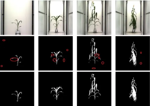
F I G U R E 6 A comparison of double-criteria thresholding (in the middle row) and segmentation using a neural network (in the bottom row) trained on the full neighborhood dataset. Areas marked in red highlight are where the neural network outperformed double-criteria thresholding
2.3
Comparison of image segmentation for
neural network and thresholding
Figure 6 contains four of the original maize images along with the corresponding segmented images obtained from using double-criteria thresholding and the neural network trained on the full NB dataset. The images from double-criteria thresholding are in the middle row and the images from the neural network are in the bottom row. The areas enclosed in red on the images in the middle row show where the neural network segmentation outperformed the double-criteria thresholding. These areas are either filled in better in the bottom row or are background pixels misclassified as plant pixels. Note that thresholds oft1=30/255 andt2=0.1 were used because they appeared to yield the best resulting images by double-criteria thresholding.
It is clear in these images that the segmentation by neu-ral network both fills in the plants and eliminates back-ground noise better. That is, both types of misclassifications— background classified as plant and plant classified as background—are reduced by using the neural network trained on the NB dataset for segmentation.
3
DISCUSSION
Aside from its good performance on the reduced training datasets, another factor in selecting the neural network trained on the NB dataset as the final classification method was com-putation time. While this method was the best one that could be trained on the available hardware, it is possible that the
ran-dom forest or even support vector machine may yield compa-rable results with more powerful computational resources. It would be of interest to compare both the segmented images from these other methods as well as the time it takes each method to segment the image. For a 384 by 384 pixel image, our neural network method takes around 8 s to predict each pixel’s class. When the image is 1000 by 1000 pixels, that time increases to approximately 1 min. The time to segment an image may be reduced by predicting using a graphics process-ing unit (GPU) rather than a central processprocess-ing unit (CPU). Distributed computing could also be used if speeding up the segmentation time is of concern in a particular application.
One issue with the NB dataset is that it introduces extra correlation. Consider a pixel around the middle of a given image. The red, green, and blue intensity values for that pixel will show up in nine rows of the dataset. While this extra correlation does not violate any assumption of a neural network, there are perhaps more elegant ways of including neighborhood information about each pixel than what was considered here. Alternatively, convolutional neural networks for segmentation (Long, Shelhamer, & Darrell, 2015) may be a fruitful approach.
Because this study has introduced a novel approach to obtaining training labels from plant images through the use of K-means, it would be of interest to construct a tool that would aid researchers in the implementation of our method. The Pixel Inspection Tool in ImageJ, for instance, returns the pixel intensity values of user-selected regions in an image (Gehan et al., 2017). A tool usingK-means for obtaining train-ing data would not need the user to manually select a region of
plant pixels. All that would be needed is a plant image cropped to contain plant and a relatively homogeneous background.
While the images shown here were all similar enough that labeled training data could be obtained, most images that are of interest for segmentation do not share the same background. For instance, it may be desirable to segment similar images of maize that are taken in a field. While numerous challenges can arise, the neural network trained for segmentation on the NB dataset has already been tested or deployed in a number of applications that are notably different from the images used in our training set. These include maize from a different green-house with different background and lighting, maize in a field, soybean [Glycine max(L.) Merr.] in a greenhouse, and images taken from directly above both maize and soybean. The results have ranged from encouraging to ready for analysis. For other traits of interest, for example segmenting the tassel of a plant, the proposed method can be applied as well. Training data for the tassel can be constructed similarly to how the training data were obtained for the rest of the plant. In more challeng-ing cases of plant segmentation, such as the field environment, our method serves as an excellent starting point, and its perfor-mance could be improved by incorporating more training data. DATA AVAILABILITY
All code along with related data are posted on Github at https://github.com/jasonradams47/PlantSegmentationCode. The raw image data used in this study are hosted at CyVerse (Liang & Schnable, 2017).
CONFLICT OF INTEREST
The authors have no competing financial interests. ORCID
Jason Adams https://orcid.org/0000-0003-2085-4911
Yumou Qiu https://orcid.org/0000-0003-4846-1263
Yuhang Xu https://orcid.org/0000-0003-4351-4602
James C. Schnable
https://orcid.org/0000-0001-6739-5527
R E F E R E N C E S
Breiman, L. (2001). Random forests. Machine Learning, 45, 5–32. https://doi.org/10.1023/A:1010933404324
Chéné, Y., Rousseau, D., Lucidarme, P., Bertheloot, J., Caffier, V., Morel, P., …Chapeau-Blondeau, F. (2012). On the use of depth camera for 3D phenotyping of entire plants. Computers and
Electronics in Agriculture, 82, 122–127. https://doi.org/10.1016/
j.compag.2011.12.007
Choudhury, S. D., Bashyam, S., Qiu, Y., Samal, A., & Awada, T. (2018). Holistic and component plant phenotyping using temporal image sequence. Plant Methods, 14, https://doi.org/ 10.1186/s13007-018-0303-x
Davies, E. R. (2012).Computer and machine vision: Theory, algorithms,
practicalities(4th ed.). Orlando, FL: Academic Press.
Fahlgren, N., Gehan, M. A., & Baxter, I. (2015). Lights, camera, action: High-throughput plant phenotyping is ready for a
close-up. Current Opinion in Plant Biology, 24, 93–99. https://doi.org/
10.1016/j.pbi.2015.02.006
Ge, Y., Bai, G., Stoerger, V., & Schnable, J. C. (2016). Tempo-ral dynamics of maize plant growth, water use, and leaf water content using automated high throughput RGB and hyperspectral imaging.Computers and Electronics in Agriculture,127, 625–632. https://doi.org/10.1016/j.compag.2016.07.028
Gehan, M. A., Fahlgren, N., Abbasi, A., Berry, J. C., Callen, S. T., Chavez, L., …Sax, T. (2017). PlantCV v2: Image analysis soft-ware for high-throughput plant phenotyping.PeerJ,5, e4088 https:// doi.org/10.7717/peerj.4088
Habier, D., Fernando, R. L., Kizilkaya, K., & Garrick, D. J. (2011). Extension of the Bayesian alphabet for genomic selection. BMC
Bioinformatics,12, https://doi.org/10.1186/1471-2105-12-186
Hamuda, E., Glavin, M., & Jones, E. (2016). A survey of image pro-cessing techniques for plant extraction and segmentation in the field. Computers and Electronics in Agriculture, 125, 184–199. https://doi.org/10.1016/j.compag.2016.04.024
Hartmann, A., Czauderna, T., Hoffmann, R., Stein, N., & Schreiber, F. (2011). HTPheno: An image analysis pipeline for high-throughput plant phenotyping. BMC Bioinformatics, 12, 148 https://doi.org/ 10.1186/1471-2105-12-148
Hastie, T., Tibshirani, R., & Friedman, J. (2009).The elements of
statis-tical learning: Data mining, inference, and prediction(2nd ed.). New
York: Springer. https://doi.org/10.1007/978-0-387-84858-7 Hsu, C.-W., Chang, C.-C., & Lin, C.-J. (2016). A practical guide
to support vector classification. Taipei, Taiwan: Department of
Computer Science, National Taiwan University. Retrieved from https://www.csie.ntu.edu.tw/~cjlin/papers/guide/guide.pdf
Johnson, R. A., & Wichern, D. W. (2002).Applied multivariate statistical
analysis(5th ed.). Englewood Cliffs, NJ: Prentice Hall.
Kingma, D. P., & Ba, J. (2014). Adam: A method for stochastic optimization. arXiv, 1412, 6980. Retrieved from https://arxiv.org/ abs/1412.6980
Klukas, C., Chen, D., & Pape, J.-M. (2014). Integrated analysis platform: An open-source information system for high-throughput plant phenotyping.Plant Physiology,165, 506–518. https://doi.org/ 10.1104/pp.113.233932
LeCun, Y., Bengio, Y., & Hinton, G. (2015). Deep learning.Nature,521, 436–444. Retrieved from https://doi.org./10.1038/nature14539 Liang, Z., & Schnable, J. (2017). Maize diversity phenotype map. [Data
set]. CyVerse Data Commons. https://doi.org/10.7946/P22K7V Lin, Y. (2015). Lidar: An important tool for next-generation
pheno-typing technology of high potential for plant phenomics?
Com-puters and Electronics in Agriculture,119, 61–73. https://doi.org/
10.1016/j.compag.2015.10.011
Long, J., Shelhamer, E., & Darrell, T. (2015).Fully convolutional
net-works for semantic segmentation(pp. 3431–3440). In Proceedings
of the IEEE conference on computer vision and pattern recognition. Red Hook, NY: Curran Associates.
McCormick, R. F., Truong, S. K., & Mullet, J. E. (2016). 3D sorghum reconstructions from depth images identify QTL regulating shoot architecture.Plant physiology,172, 823–834. https://doi.org/ 10.1104/pp.16.00948
Miao, C., Yang, J., & Schnable, J. C. (2019). Optimising the identi-fication of causal variants across varying genetic architectures in
crops.Plant Biotechnology Journal,17, 893–905. https://doi.org/ 10.1111/pbi.13023
Miller, N. D., Parks, B. M., & Spalding, E. P. (2007). Computer-vision analysis of seedling responses to light and gravity.The Plant Journal,
52, 374–381. https://doi.org/10.1111/j.1365-313X.2007.03237.x Otsu, N. (1979). A threshold selection method from gray-level
his-tograms.IEEE Transactions on Systems, Man, and Cybernetics,9, 62–66. https://doi.org/10.1109/TSMC.1979.4310076
Peñuelas, J., & Filella, I. (1998). Visible and near-infrared reflectance techniques for diagnosing plant physiological
sta-tus.Trends in Plant Science,3, 151–156. https://doi.org/10.1016/
S1360-1385(98)01213-8
Scharr, H., Minervini, M., French, A. P., Klukas, C., Kramer, D. M., Liu, X.,…Tsaftaris, S. A. (2016). Leaf segmentation in plant phe-notyping: A collation study.Machine Vision and Applications,27, 585–606. https://doi.org/10.1007/s00138-015-0737-3
Sezgin, M., & Sankur, B. (2004). Survey over image thresholding tech-niques and quantitative performance evaluation. Journal of
Elec-tronic Imaging,13, 146–166. https://doi.org/10.1117/1.1631315
Suykens, J. A. K., & Vandewalle, J. (1999). Least squares support vector machine classifiers.Neural Processing Letters,9, 293–300. https:// doi.org/10.1023/A:1018628609742
Vibhute, A., & Bodhe, S. K. (2012). Applications of image processing in agriculture: A survey.International Journal of Computer
Applica-tions,52(2), 34–40. https://doi.org/10.5120/8176-1495
Wager, S., Wang, S., & Liang, P. S. (2013). Dropout training as adap-tive regularization. In C. J. C. Burges, L. Bottou, M. Welling, Z. Ghahramani, & K. Q. Weinberger (Eds.),Advances in Neural
Information Processing Systems 26(pp. 351–359). Red Hook, NY:
Curran Associates.
Wahba, G. (1999). Support vector machines, reproducing kernel Hilbert spaces and the randomized GACV. In B. Schölkopf, C. J. C. Burges, & A. J. Smola (Eds.),Advances in Kernel Methods: Support Vector
Learning(pp. 69–87). Cambridge, MA: MIT Press.
Xavier, A., Hall, B., Casteel, S., Muir, W., & Rainey, K. M. (2017). Using unsupervised learning techniques to assess interactions among complex traits in soybeans.Euphytica,213, 200. https://doi. org/10.1007/s10681-017-1975-4
Xiong, X., Yu, L., Yang, W., Liu, M., Jiang, N., Wu, D., … Liu, Q. (2017). A high-throughput stereo-imaging system for quantify-ing rape leaf traits durquantify-ing the seedlquantify-ing stage.Plant Methods,13, https://doi.org/10.1186/s13007-017-0157-7
How to cite this article: Adams J, Qiu Y, Xu Y, Schnable JC. Plant segmentation by supervised machine learning methods.Plant Phenome J. 2020;3:e20001.https://doi.org/10.1002/ppj2.20001