Occurrence of Compact Groups of Galaxies through Cosmic Time

Typeset using L_TEXtwocolumnstyle withlikeapj1.1

The Occurrence of Compact Groups of Galaxies Through Cosmic Time

Liting Xiao1, 9

1_{Department of Astronomy, University of Virginia, P.O. Box 400325, Charlottesville, VA 22904-4325, USA} 2_{National Radio Astronomy Observatory, 520 Edgemont Road, Charlottesville, VA 22903, USA}

3_{Astrophysics Science Division, Laboratory for X-ray Astrophysics, NASA/Goddard Space Flight Center, Mail Code 662, Greenbelt, MD 20771, USA} 4_{CRESST, University of Maryland Baltimore County, 1000 Hilltop Circle, Baltimore, MD 21250, USA}

5_{Department of Physics and Astronomy, University of Western Ontario, London, ON N6A 3K7, Canada} 6_{Centre for Planetary and Space Exploration, University of Western Ontario, London, ON N6A 5B9, Canada}

7_{Rotman Institute of Philosophy, University of Western Ontario, London, ON N6A 5B9, Canada} 8_{Canadian Space Agency, Saint-Hubert, QC J3Y 8Y9, Canada}

9_{Division of Physics, Mathematics and Astronomy, California Institute of Technology, Pasadena, CA 91125, USA}

Received ; revised ; accepted 2019; published

Abstract

We use the outputs of a semi-analytical model of galaxy formation run on the Millennium Simulation to investigate the prevalence of three-dimensional compact groups (CGs) of galaxies fromz=11 to 0. Our publicly available code identifies CGs using the 3D galaxy number density, the mass ratio of secondary+tertiary to the primary member, mass density in a surrounding shell, the relative velocities of candidate CG members, and a minimum CG membership of three. We adopt “default” values for the first three criteria, representing the observed population of Hickson CGs atz=0. The percentage of non-dwarf galaxies (M>5_×108h−1M) in CGs peaks nearz_∼2 for the default set, and betweenz_∼1₋3 for other parameter sets. This percentage declines rapidly at higher redshifts (z_&4), consistent with the galaxy population as a whole being dominated by low-mass galaxies excluded from this analysis. According to the most liberal criteria, _.3% of non-dwarf galaxies are members of CGs at the redshift where the CG population peaks. Our default criteria result in a population of CGs atz<0.03 with number densities and sizes consistent with Hickson CGs. Tracking identified CG galaxies and merger products toz=0, we find that.16% of non-dwarf galaxies have been CG members at some point in their history. Intriguingly, the great majority (96%) ofz=2 CGs have merged to a single galaxy byz=0. There is a discrepancy in the velocity dispersions of Millennium Simulation CGs compared to those in observed CGs, which remains unresolved.

Key words:galaxies: statistics, galaxies: groups: general, galaxies: evolution, galaxies: interactions

1. Introduction

Determining which physical mechanisms dominate the pro-cessing of gas in galaxies is at the core of understanding galaxy evolution over cosmic time. With high apparent galaxy number densities and relatively low velocity dispersions (Hickson et al.

1992; Mamon1992), compact groups of galaxies (CGs) appear to be the ideal environment to investigate how gas processing is impacted by relatively strong interactions between multiple galaxiessimultaneously.

Recent work has demonstrated that the compact group en-vironment has an impact on galaxy evolution that is not seen in several other environments including field galaxies, isolated pair-wise mergers, or galaxy clusters (Johnson et al. 2007; Tzanavaris et al.2010; Walker et al.2010,2012; Lenki´c et al.

2016; Zucker et al. 2016). Specifically, galaxies that reside in CGs exhibit a “canyon” in infrared color space that implies a rapid transition between relatively actively star-forming and quiescent systems. Curiously, it should be noted that this tran-sition region in infrared color space corresponds to the opti-cal “red sequence” rather than the “green valley” (Walker et al.

2013; Zucker et al.2016), indicating that a distinct evolution-ary process is taking place in CGs. In other words, the infrared transition region seen in CGs, is not seen in comparison sam-ples and should not be confused with the optical green valley.

This is further corroborated by a bimodality in star formation rates normalized by stellar mass (specific star formation rates,

sSFRs), which is particular to the CG environment (Tzanavaris et al. 2010; Lenki´c et al.2016), although some bimodal be-havior has been reported in loose groups as well (Wetzel et al.

2012). Bimodal star formation suppression was also reported by Alatalo et al. (2015) who studied warm H2gas in CGs (see also Cluver et al.2013). Peculiar sSFR behavior was also re-ported by Bitsakis et al. (2010,2011), who found that late type galaxies in CGs have systematically low specific star forma-tion rates. Lisenfeld et al. (2017) found that some CG galaxies appear to have a lower star-formation efficiency (SFR/MH2); however, star-forming compact group galaxies do lie on the star-forming main sequence, consistent with galaxies in other environments (Lenki´c et al.2016).

A number of other works have shown that galaxy evolution is impacted by the compact group environment. Proctor et al. (2004), Mendes de Oliveira et al. (2005), and Coenda et al. (2015) found that CG galaxies tend to be older (in terms of the average age of their stellar populations) than galaxies in other environments. Coenda et al. (2012) found a significantly larger fraction of red and early-type galaxies in CGs, as com-pared to loose groups, while Mart´ınez et al. (2013) established that brightest group galaxies in CGs are brighter, more massive, larger, redder and more frequently classified as elliptical com-pared to their counterparts in loose groups. Coenda et al. (2015) found that CGs include a late-type population with markedly reduced sSFRs than loose groups and field populations. The

fraction of quiescent galaxies (i.e., not actively star-forming, in-dependent of the average age of the stellar population) in CGs is higher than in the field or loose-group population (Coenda et al.2015; Lenki´c et al.2016).

Farhang et al. (2017) compared CGs to fossil groups in the Millennium Simulation, finding that some, but not all, CGs eventually turn into fossil systems. They stressed that CGs ap-pear to be a distinct group environment.

The fact that CGs show distinct features and/or behavior when compared to other environments suggests that the CG environment is “doingsomething” that impacts galaxy evolu-tion in a unique way, not prevalent in other environments. In turn, this may be linked to the high, present or past, interac-tion activity experienced by galaxies in these systems (e.g., see the detailed results on interactions in CG systems in Plana et al.

1998; Mendes de Oliveira et al.1998,2003; Amram et al.2004; Torres-Flores et al.2009,2010,2014).

The importance of understanding how galaxy evolution is im-pacted by the group environment is underscored by the fact that most galaxies spend the majority of their time in groups of some kind (e.g. Mulchaey2000; Karachentsev2005, and ref-erences therein). However, the fraction of galaxies that have been part of a compact group over cosmic time is unclear, and therefore the total impact of the compact group environment on galaxy evolution throughout the Universe has not been well constrained. Catalogs of CGs are restricted to the relatively nearby Universe (e.g., Hickson et al.1992; Barton et al.1996; Lee et al.2004; Deng et al. 2007; McConnachie et al.2009; D´ıaz-Gim´enez et al.2012; but see Pompei & Iovino2012) and even in these cases CGs can only be confirmed if velocity in-formation is available for the constituent galaxies. For exam-ple, the Redshift Survey Compact Group catalog (Barton et al.

1996) has a magnitude limit ofmB<15.5, only reaching a red-shift ofz_.0.03. Advances in galaxy simulations over the last decade now enable us to explore the prevalence of CGs out to arbitrarily high redshifts.

1.1. Simulations

As it is not possible to observe a sample of CGs spanning all redshifts, the only available path forward is to utilize cos-mic simulations of galaxy evolution. The Millennium Simula-tion (Springel et al.2005; Lemson & Virgo Consortium2006) provides a tool to study the history of CGs in the Universe. It used 21603 particles with mass M =8.6_×108h−1M to trace the evolution of a comoving cube with side-length 500h−1

Mpc, wherehis the Hubble constant parametrization such that

H0=100hkm s−1Mpc−1. The Millennium Simulation used a ΛCDM model with cosmological parameters ΩM =0.25, Ωb=0.045, ΩΛ=0.75, and h=0.73, consistent with

obser-vational results from the Carnegie Hubble Program (Freedman et al.2012) as well as the WMAP (Hinshaw et al.2013) mis-sion1_.

The Millennium Simulation used only dark matter particles to which associated properties were later assigned. Dark mat-ter halos were identified using a friends-of-friends algorithm as described in Springel et al. (2005). Galaxies were added to the simulationpost facto using semi-analytic techniques (e.g. De 1_{In this paper all distances and masses are scaled toh=1.}

Lucia & Blaizot2007; Guo et al.2010,2011,2013). Galaxies are initially associated with individual dark matter halos, which may become subhalos of larger structures over time. The tech-niques of De Lucia & Blaizot (2007), for example, expanded on the methods of Croton et al. (2006) and incorporated the effects of rapid star formation and gas loss in galaxy mergers, changes in galaxy properties with varying stellar mass functions and stellar populations, and attenuation due to dust.

The simulation results were saved in a collection of 64 red-shift “snapshots”. The identified dark matter halos were then assigned galaxy properties using the semi-analytic techniques discussed in the references above. The snapshots combined with the high resolution of the simulation and the sophisticated semi-analytic galaxy formation and evolution models, provide an excellent tool for studying the history of CGs over cosmic time. Throughout this paper, we adopt the De Lucia & Blaizot (2007) catalog of galaxies created through this semi-analytic approach.

1.2. Previous Work

A number of previous studies have utilized the Millennium Simulation galaxy catalogs to investigate CGs. These studies have been limited to relatively low redshifts to facilitate com-parison to observations, such as the well-known Hickson cat-alog (Hickson 1982; Hickson et al. 1992). By using a light cone in the Millennium Simulation galaxy catalogs (Henriques et al.2012), it has also been possible to create “mock” cata-logs of CGs, which can be compared to observations and are subject to analogous limitations (e.g., interloping foreground or background galaxies, McConnachie et al.2008; D´ıaz-Gim´enez & Mamon2010; D´ıaz-Gim´enez & Zandivarez2015; Farhang et al.2017).

By comparing mock CGs in projection in the Millennium Simulation to observed Hickson Compact Groups (HCGs), Mc-Connachie et al. (2008) found that_∼29% of mock CGs identi-fied from “images” alone are physically dense systems of three or more galaxies, and that the remaining projected CGs are re-sults of chance alignments. D´ıaz-Gim´enez & Mamon (2010) found that the fractions of 3D dense groups among 2D com-pact groups depends on the semi-analytical model (SAM) used, the consideration of galaxy blending and the criterion used to define a dense group. Their Table 5 indicates that, for particle-based group definitions and their optimal definition of a dense group combining line-of-sight size and elongation, the frac-tions of compact groups selected in projection that are physi-cally dense range from 20% for the De Lucia & Blaizot (2007) SAM, to 43% for the Bower et al. (2006) SAM. These fractions rise to over half and up to 3/4, respectively, for CGs that sur-vive the velocity filter. The differences with the results from the McConnachie team arise from different definitions of what constitutes a physically dense group.

Finally, by comparing CGs observed in the 2MASS catalog to those in a mock light-cone from a Millennium Simulation galaxy catalog, D´ıaz-Gim´enez & Zandivarez (2015) found that only about a third of CGs are embedded in larger structures, i.e., the majority are truly isolated systems; yet D´ıaz-Gim´enez & Mamon (2010) find that only 11% of their velocity-filtered CGs are constituted by the Friends-of-Friends group in 3D, hence are isolated.

Retrieve simulation chunk

DBSCAN clustering algorithm

Remove dwarf and “fly-by” galaxies

Filter clusters to identify compact groups

Save group and member statistics

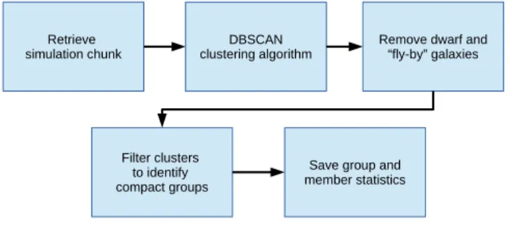
Figure 1. The algorithmic process developed for obtaining and ana-lyzing Millennium Simulation galaxy catalogs.

2. Identification of Compact Groups in the Millennium Simulation Galaxy Catalogs

Identifying CGs with robust criteria has presented a chal-lenge to investigators in a number of studies, and the result-ing group demographics are sensitive to these criteria (Geller & Postman e.g.1983; Nolthenius & White e.g.1987; see also Table 5 in D´ıaz-Gim´enez et al.2012, Taverna et al.2016and references therein). Here we invoke an algorithm with a set of tunable parameters that allows us to investigate how the de-mographics of a compact group sample depend on individual parameters.

2.1. Algorithm

We developed an open-source, publicly available code2 to identify and characterize CGs in Millennium Simulation galaxy catalogs. This process is sub-divided into several simple al-gorithms with tunable parameters defining the properties of galaxy groups considered “compact”, where we use “compact” to refer to the 3D spatial separation. The general outline of our methodology (see also Figure1) is as follows:

1. Download galaxy data from a chunk (snapshot at a given redshift) of the Millennium Simulation, utilizing the De Lucia & Blaizot (2007) catalog;

2. Use a tunable clustering algorithm to identify clusters and groups of galaxies in the simulation chunk;

3. Filter out identified group members which are dwarf or “fly-by” galaxies;

4. Measure statistics of the discovered galaxy groups; 5. Use tunable parameters to filter the identified galaxy

groups to select only “compact groups”;

6. Save the statistics of identified compact groups and their galaxy members.

These algorithms contain several tunable parameters that can be used to adjust how CGs are selected from the Millennium Simulation galaxy data. These are briefly outlined here, and described in greater detail in the following sections:

2 _{https://github.com/cdw9bf/CompactGroup}

• Neighborhood,NH– the neighborhood parameter of the DBSCANalgorithm (similar to the “linking length” pa-rameter of friends-of-friends algorithms);

• Minimum number of members, Nmin– the minimum number of non-dwarf galaxy members an identified can-didate group must have in order to be considered a com-pact group;

• Maximum shell density ratio,SR– the maximum allow-able ratio of the virial mass3 density of galaxy subhalos in a shell surrounding a compact group to the virial mass density of galaxy subhalos within that compact group;

• Galaxy mass ratio, MR– the minimum allowable virial-mass ratio of the secondary+tertiary dark matter subhalos to the primary galaxy dark matter subhalos in a group;

• Critical velocity difference,_|∆v_|– the velocity difference between a galaxy and the median velocity of a compact group for the galaxy to be considered a “fly-by” and not a member of the compact group;

• Dwarf limit – the stellar mass limit for a galaxy to be considered a dwarf galaxy and thus excluded from con-sideration.

2.2. Tunable Clustering Algorithm

To identify clusters and groups of galaxies, we used DB-SCAN, which employs an intuitive, number density-based clus-tering approach (Ester et al.1996). DBSCANis very adept at handling arbitrary shapes as it does not depend on any density-smoothing processes. In clustering terminology, each galaxy constitutes a “node”. The algorithm works by searching the de-fined radial neighborhood of each node and counting the num-ber of neighbors that are within this radius. If the neighborhood contains more than, or equal to, the minimum number of mem-bers, then it is flagged. This is repeated for each node/member until all nodes within the neighborhood have been searched, thus classifying the resulting flagged collection of nodes as a “cluster” (Birant & Kut2006), which in our case is an identi-fied compact group. The group’s center is defined as the median of the positions of the identified galaxy members. The group ra-dius is then the greatest distance from this center to any of the member galaxies.

Thus, DBSCAN requires two initial parameters,

neighbor-hoodandminimum number of members. Neighborhoodis the

radius starting on each identified node and used to search for adjacent nodes. Minimum number of membersspecifies the re-quired minimum number (density) of galaxies that are in the neighborhood of an identified node (a “central” galaxy), for the system to be considered a compact group.

One caveat about the DBSCANalgorithm is that is only de-terministic under certain conditions. The minimum number of members must be less than or equal to three. If this condition is met, which it is in this study, then the algorithm is fully de-terministic.

3 _{Virial mass is defined in De Lucia & Blaizot (2007) as the number of}

2.3. Properties of Hickson Compact Groups

We selected our CGs in 3-D space from the semi-analytical model outputs in a similar manner as Hickson selected his CGs in redshift space. The selection criteria Hickson used were based on compactness, relative luminosity, minimum number of members, and isolation. The particular parameters were cho-sen to identify dense systems of multiple galaxies while exclud-ing substructure within galaxy clusters.

Using imaging alone, Hickson (1982) defined his compact groups with a membership of at least four galaxies (although subsequent studies relaxed this restriction to three members; Barton et al.1996). The requirement for compactness was that the surface brightness averaged over the smallest circle enclos-ing the group galaxy centers be brighter than 26 mag arcsec−2. The isolation criterion was that there should be no galaxies brighter than the faintest galaxy within 3 times the angular ra-dius of the group. This aimed to exclude CGs that are asso-ciated with galaxy clusters or other regions whose “external” galaxies may strongly influence group galaxies. As these re-strictions are subject to projection effects, the presence of fore-ground or backfore-ground galaxies can influence the initial identifi-cation of CGs (by falsely including or excluding them, Mamon

1986; McConnachie et al. 2008; Brasseur et al. 2009; D´ıaz-Gim´enez & Mamon2010).

In addition, the spectroscopic study of Hickson et al. (1992) introduced the further criterion that an “accordant” member galaxy should be within 1000 km s−1of the median group ve-locity. This criterion was meant to remove distant foreground and/or background galaxies that appear in projection along the line of sight.

2.4. Selection Criteria

Our selection criteria were motivated by those used for Hick-son’s original catalog, modified to take full advantage of the three-dimensional information in the Millennium Simulation galaxy catalogs produced by the semi-analytical model of De Lucia & Blaizot (2007).

We describe subsequently in this section our choices for the input parameter values to DBSCANbased on the known proper-ties of HCGs that have been determined empirically since their identification. TheNHparameter is the search radius around a galaxy, effectively determining the degree of group compact-ness, and is the initial parameter used by the DBSCAN algo-rithm to identify clustered galaxies.SRis a group isolation cri-terion, whileMRis a criterion characterizing the dominance of the most massive galaxy in a group among the top-ranked group galaxies.

2.4.1. Neighborhood Parameter:NH

The groups that were identified as HCGs have a median 2-D galaxy-galaxy separation of 39h−1kpc (Hickson et al.1992). This separation between galaxies is related to the compactness selection criterion, since CGs have to have a surface bright-ness of at least 26 mag arcsec−2 (Hickson1982). Note that the galaxy separation is projected from 3-D space down to 2-D space, and therefore underestimates the intrinsic separation of galaxies in a group. To find the 3-D correction factor, we per-formed a Monte Carlo simulation in which we constructed 106 realizations of galaxies, randomly positioned in 3-D space. The

median distance between galaxies was measured in 2-D space for each realization. We find that the median 3-D distance be-tween galaxies is roughly 2π/5 larger than the projected 2-D distance. Based on the median projected distance and the mul-tiplier, we estimate the median separation between HCG galax-ies in 3-D space to be about 50h−1kpc. This directly relates to the neighborhood parameter (NH) in the DBSCAN algorithm. We adoptNH=25,50,and 75h−1kpc to bracket the empirical value.

2.4.2. Minimum number of members: Nmin

There is no consensus in the literature regarding the min-imum number of member galaxies for a candidate compact group. The original Hickson (1982) criterion was Nmin =4, and this was adopted by a number of works (e.g. McConnachie et al.2008; D´ıaz-Gim´enez & Zandivarez2015). On the other hand, several studies have included triplets (Nmin=3, e.g. Bar-ton et al.1996; Tzanavaris et al.2010; Lenki´c et al.2016). We choose to include triplets as a more general lower limit for the number of CG member galaxies. We do not varyNmin, as this would be a separate full study, the computational demands of which are well beyond this paper. For reference, we note that among our selected candidate CGs, the fractions of systems that are triplets are 61.5% atz_∼2, and 68% atz=0.

2.4.3. Limit on Mass in Surrounding Shell:SR

In order to select against groups that might be associated with larger clusters, we invoke a maximum stellar mass-density re-quirement for a shell surrounding a compact group. Specifi-cally, the ratio of the stellar mass density within the surround-ing shell to the stellar mass density of the compact group, SR≡ρshell/ρgrp, must be less than a threshold value. In other words, we compare the stellar mass density (as determined from the combined virial masses of the constituent galaxy sub-halos) in a shell around an identified group to the stellar mass density of the group’s identified member galaxies. We choose threshold values of log(SR)=₋3,₋4 and₋5.

Initially, we adopted a shell radial width that was a multiple of the group radius, aiming to mimic the Hickson (1982) iso-lation criterion, since that was dependent on a group’s angular radius. However, this led to many selected groups that were in fact located within galaxy clusters. The likely explanation for this is that some group radii were so small that multiplying them by a small factor did not adequately sample the local en-vironment. Instead, we opted to use a fixed radial width based on 1) the distance beyond which quenching is not observed in dwarf galaxies (>1.5 Mpc, Geha et al.2012), and 2) the cur-rent distance between the Milky Way and Andromeda Galaxies (_∼0.8 Mpc), which roughly defines the “core” of the Local Group. Based on these two empirical benchmarks, we adopt an intermediate shell radial width of 1h−1Mpc extending beyond the identified group radius.

Because we use the mass density at a fixed radius, we also exclude any group within 1h−1Mpc from the edges of the box in each chunk due to the fact that some volume of the sphere outside of the cube is inherently empty and skews the ratio to-wards a less dense environment.

In order to select against groups that consist of a single mas-sive galaxy with small satellites, Hickson (1982) required that constituent galaxies have magnitudes within 3 magnitudes of the brightest member. This requirement also helps to mitigate against galaxies that only appear to be members of the group due to projection effects, but are in fact at very different dis-tances. In the Millennium Simulation galaxy catalogs all spatial relationships between galaxies are known, ensuring that projec-tion effects do not contaminate the sample. Another advantage of the Millennium Simulation is that it provides masses of the galaxy subhalos from galaxy catalogs that allowed us to directly compare the masses instead of relying on observables such as apparent magnitude (De Lucia & Blaizot2007). As a result, we are much less sensitive to the specific prescriptions for star formation within the semi-analytical modeling, and our results should be generalizable to other galaxy catalogs based on the Millennium Simulation.

We make the assumption that dominance in galaxy luminos-ity corresponds to dominance in galaxy and subhalo mass. In order to select against groups that consist of a single dominant galaxy with minor satellites, we required a minimum, thresh-old value for the mass ratio of the combined mass of the sec-ond and third most massive galaxies to that of the most massive galaxy, defined asMR≡(Msecondary+Mtertiary)/Mprimary. While this requirement still allows for “minor” galaxy companions, it excludes systems similar to the Milky Way and its satellites. The advantage of this method, as opposed to a hard cutoff in galaxy subhalo mass, is that it allows less luminous galaxies to be members of a compact group as long as they are sufficiently massive. We choose minimum threshold values ofMR=0.20, MR =0.10 and MR =0.05; a three-“magnitude” mass ratio would correspond toMR=0.06.

2.4.5. Relative Velocity Restriction

To avoid identifying galaxies as members of a compact group that are not subject to a long-term dynamical interaction, we introduce a velocity filter. This filter eliminates any galaxies that have_|∆v|>1000 km s−1from the median group velocity, and is the velocity filter that was used by Hickson et al. (1992). We find that this only excludes 1.6% of potential CGs. We note that for observational studies, galaxies with peculiar velocities could appear to have accordant velocities, but still potentially not be physically associated with a group. Given that all spatial relationships are known for the galaxies in this work, group members are not subject to this caveat.

2.4.6. Exclusion of Dwarf Galaxies

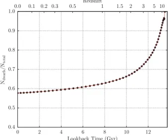
In our analysis we impose a galaxy mass threshold to exclude galaxies with stellar masses that may be too low. Specifically, only galaxies that have masses greater than 5_×108h−1Mare included. This corresponds to a median dark matter halo mass of 3.4_×1010M or _∼40 dark matter particles. Any “galax-ies” with zero stellar mass are also removed from the analysis as they are artifacts of the De Lucia & Blaizot (2007) semi-analytical model. As shown in Figure2, even for redshifts of

z_.0.5, this results in the exclusion of_∼60% of the mass sys-tems identified in the Millennium Simulation galaxy catalog. At earlier cosmic times, the relative fraction of such “dwarf”

galaxies that are excluded due to this mass cut-off becomes in-creasingly important, reaching more than 80% atz&5.

✵ ✷ ✹ ✻ ✽ ✶✵ ✶ ✷ ▲♦♦❦ ❜❛❝❦❚✐♠❡✭●② r ✮ ✵✿ ✹ ✵✿✺ ✵✿ ✻ ✵✿✼ ✵✿✽ ✵✿✾ ✶✿✵ ◆ ❞ ✇ ✁ ❢ s ❂ ◆ t ✂ t ❧ ✵✳✵ ✵✳✶ ✵✳✷ ✵✳✸ ✵✳✺ ✶ ✶✳✺ ✷ ✸ ✺ ✶✵ ❘ ❡✄☎❤✐ ✆ ✝

Figure 2. Evolution of the fraction of “dwarf” galaxies (stellar mass

<5_×108h−1M) identified in the De Lucia & Blaizot (2007) semi-analytical model of galaxy formation run on the Millennium Simula-tion. These systems are excluded from further analysis for the rea-sons discussed in§2.4.6. The exclusion of dwarf galaxies results in a lower limit on the number of identified CGs that becomes increas-ingly more significant at higher redshift. Forz<0.5, the fraction of excluded galaxies based on the mass criterion is.60%. The fraction rises rapidly forz>1. See §2.4.6for further discussion.

2.4.7. Significance of Selection Criteria

In order to both mitigate the effect of a set of rigid selection criteria and also investigate how compact group demographics may depend on these criteria, we varyNH, SRandMR over a range of values about a “default” set (see Table1). We first test each non-default value by keeping all other criteria at their de-fault values, and then also use combinations of most “lenient” and most “restrictive” parameter values, in order to constrain the most extreme CG populations. In the case ofNH, lower val-ues reduce the size of the search area for neighboring galaxies, so that more compact groups will be selected, and conversely for higher values. For very large values, galaxy clusters will start to be included. Our default value is 50h−1kpc (see Sec-tion2.4.1), and we also use the values 25 and 75h−1kpc.

Our default value for log(SR) is₋4, and we also use₋3 and

−5. ForMRthe default value is 0.10, and we also use 0.05 and 0.20.

3. Processing Algorithm 3.1. Optimization Strategy

To be able to analyze the full simulation in a time-efficient manner, we developed optimization strategies. The resulting time requirements are extreme: the full simulation catalog has over 26 million galaxies in its most populous snapshot. In or-der to make the algorithm more computationally efficient, we

divide a given snapshot into roughly equivalent overlapping boxes. Each box has a side length of 102h−1Mpc correspond-ing to about 1/125 of the total simulation volume. Only the central 100h−1 Mpc were sampled in each box, since, when conducting the density analysis, a buffer zone of 1h−1Mpc is needed at the edge. Without this buffer, the groups on the edge of the box would contain less volume in the spherical density analysis than required to determine a group’s isolation. This process of division allowed us to run the algorithm in an exten-sively parallelized fashion on as many cores as desired.

3.2. Tracking Galaxies Through the Simulation

To track the galaxies in any snapshot that are, or have ever been, in CGs, each galaxy had to be monitored throughout the simulation. The Millennium Simulation employs a stan-dard naming convention for galaxies, and also provides the de-scendant ID. Once the groups are identified in the main algo-rithm, they can then be traced through the simulation forwards or backwards in time to determine the fraction of galaxies living in CGs at any given time step.

Starting from the beginning of the simulation (cosmic time= 0), galaxies and their descendants are placed into a list, which is then searched for repeated galaxies (e.g., when a galaxy merges with another one). This process is repeated for every galaxy in a given treeID. The latter is a grouping assigned by De Lucia & Blaizot (2007) to categorize related groups of galaxies, so that all galaxies in a given compact group will have the same treeID. By dividing the data set according to treeID, further extensive parallelization was achieved.

4. Results

In this section, we present the results of multiple trials using different parameter sets and describe how the adopted selection criteria affect compact group properties and demographics. Ta-ble1 presents the grid of parameter sets and resulting group properties, as well as some key observational HCG properties for comparison.

4.1. Impact of Parameters on Group Properties

4.1.1. Mass Ratio of Group

The restriction on the mass ratio of secondary+tertiary to pri-mary galaxies (MR) has a strong impact on the fraction of galax-ies considered to be in CGs atz.5. A mass ratio ofMR=0.05 is the most lenient value, and thus results in the largest fraction of galaxies in CGs. Conversely,MR=0.20 is the most restric-tive and reduces the relarestric-tive number of galaxies considered to be in a compact group by nearly an order of magnitude forz<5 (see Figure3). All three values ofMRresult in the fraction of galaxies in CGs peaking betweenz_∼1.5₋2.4, with the more restrictive values ofMRpeaking at higher redshifts. The most liberal value ofMR = 0.05 (with other parameters set to their default values, set E) results in a maximum fraction of galaxy membership in CGs of_∼1.3%.

4.1.2. Shell Density Ratio

Varying the shell density ratio (SR) selection criterion re-sulted in similar patterns to those seen with respect to changing MR. Despite varyingSRby two orders of magnitude, the result-ing impact on the fraction of galaxies in CGs is not as strong

as seen from only changingMRby a factor of four. However, forz<5 different values ofSR do strongly influence compact group selection (Figure4). For the most restrictive (i.e., most isolated) value of log(SR)=−5 (model D), the relative number of galaxies in CGs never reached values greater than_∼0.3%. The most liberal value of log(SR)=−3, with other parameters at their default values (Model C), results in a peak fraction of galaxies in CGs of_∼0.83% atz=1.9.

4.1.3. Neighborhood

Variations in the neighborhood parameter (NH) also had a strong impact on the demographics of CGs identified in the sim-ulation. As discussed in Section4.3, a value ofNH =50h−1

kpc is found to produce groups that have similar median sizes to HCGs, whileNH=25h−1kpc andNH=75h−1kpc result in median group sizes that are smaller and larger, respectively, than observed HCGs.

4.1.4. Most Lenient and Restrictive Parameter Sets

In addition to varying individual selection parameters while holding the rest constant at their “default” values, we also test combinations of the most lenient and most restrictive parameter values in order to constrain the most extreme populations of CGs. The most restrictive criteria used here are log(SR)=₋5, MR=0.20, andNH=25h−1kpc. The most liberal values are log(SR)=₋3,MR=0.05, andNH=75h−1kpc. As shown in Figure6, even the most lenient set of criteria only result in the relative population of galaxies in CGs peaking at_∼3.1% near a redshift ofz_∼1.5.

4.2. Total Fraction of Galaxies in Compact Groups

In addition to the relative number of galaxies that are in CGs at any given redshift, we can also determine the relative number of galaxies that arecurrentlyin or haveeverbeen members of a compact group over cosmological time.

Here, we track the galaxies that are in a compact group at any given instant and continue to count them as part of the total number of galaxies as the groups evolve, even if they should no longer be considered to belong to a compact group due to mergers of constituent galaxies causing the group to have fewer than three members. By tracking the CGs’ descendants, we can determine the number and properties of galaxies in the present day that once were a part of a compact group in their evolution-ary history.

As shown in the right panel of Figure6, the maximal fraction of galaxies in the present day Universe that have ever been part of a CG exceeds 10 percent. Unlike the rest of the parameter sets, the most lenient and most restrictive ones lead to a par-ticularly large variation in the final percentage. The final per-centages range from 0.4% to 16.1% across the full parameter range.

As can be seen in the right panels of Figures3and5, both of theMRandNHcriteria have a moderate effect on the final frac-tion. On the other hand, the right panel of Figure4shows that theSRcriteria have little effect on the final fraction of galaxies that have ever been in CGs.

Finally, we trace the evolution ofz=2 CGs down toz=0. We find that the overwhelming majority (16071 out of 16797 CGs, or 96%) have merged into a single galaxy byz=0. The

0 2 4 6 8 10 12 Lookback Time (Gyr)

10−4 10−3 10−2 F raction of Galaxies in Compact Groups mr=0.05 mr=0.10 mr=0.20 0.0 0.1 0.2 0.3 0.5 Redshift1 1.5 2 3 5 10 0 2 4 6 8 10 12

Lookback Time (Gyr) 10−3 10−2 10−1 F raction of Galaxies that ha ve ev er b een in Compact Groups mr=0.05 mr=0.10 mr=0.20 0.0 0.1 0.2 0.3 0.5 Redshift1 1.5 2 3 5 10

Figure 3. Fraction of galaxies (stellar mass greater than 5_×108h−1M) living in compact groups (left) or that ever lived in one (right). Each analysis uses a neighborhood parameterNH= 50h−1kpc and a maximum shell density ratio log10(SR) =−4. These curves are the results of

varying the mass ratio (MR=0.05, red circles;MR=0.10, orange squares;MR=0.20, yellow triangles). The width of the shaded region is 50 times the Poisson uncertainty. In all cases, the fractions of galaxies in compact groups peak atz∼1.0–2.4, and drop off sharply atz∼5 because of our dwarf galaxy cutoff mass. As expected, the most restrictive value ofMR=0.20 (with top-ranked galaxies of more comparable masses) results in fewer compact groups at all redshifts.

0 2 4 6 8 10 12

Lookback Time (Gyr) 10−4 10−3 10−2 F raction of Galaxies in Compact Groups log(sr)=-3 log(sr)=-4 log(sr)=-5 0.0 0.1 0.2 0.3 0.5 Redshift1 1.5 2 3 5 10 0 2 4 6 8 10 12

Lookback Time (Gyr) 10−3 10−2 10−1 F raction of Galaxies that ha ve ev er b een in Compact Groups log(sr)=-3 log(sr)=-4 log(sr)=-5 0.0 0.1 0.2 0.3 0.5 Redshift1 1.5 2 3 5 10

Figure 4. Same as Figure3but varying the maximum shell density ratio. Each analysis uses a neighborhood parameterNH=50 h−1kpc and a minimum mass ratioMR=0.10. These curves are the results of varying the maximum shell density ratio (log(SR) =−3, red circles; log(SR) =−4, orange squares; log(SR) =−5, yellow triangles). The width of the shaded region is 50 times the Poisson uncertainty. Though the overall shapes of the curves are similar to those in Figure3, varying the values ofSRby two orders of magnitude did not produce as strong as effect as varyingMR

by a factor of 4. A restrictiveSRvalue of₋5 (indicating very isolated systems) led to the fewest CG galaxies at all redshifts.

distribution of these galaxies atz=0 in color-magnitude space is shown in Figure7. Taken at face value, this color-magnitude distribution is notably different from the general Sloan Digital Sky Survey (SDSS) sample presented by Blanton et al. (2005); the compact group descendants show a clump of red and lumi-nous galaxies, and two distinct plumes that are not seen in the general SDSS population. However, we caution that there is no guarantee that the semi-analytic model used will in general reproduce the colors of the SDSS population. Perhaps not sur-prisingly, this distribution is more similar to that observed for galaxies in compact groups (Walker et al.2013), but there re-main clear differences – including the plume of compact group descendants across a range ing₋rcolor at anI-band magnitude

of_{∼ −}23. However, the caveat that applies to SDSS colors still applies here. Thus, these results tentatively and qualitatively suggest that the products of compact group evolution may have properties statistically distinct from the general galaxy popula-tion, which warrants an in-depth follow-up study.

Interestingly, we also identify a small minority of CGs (49 out of the 726 that have not merged by z=0) that have at least one galaxy separated by 250 kpc, or more, from other group members. Such member galaxies are reminiscent of NGC 7320C, located in the northeast quadrant of Stephan’s Quintet (HCG 92) and likely to have passed through the group a few times_∼108years ago. It has been suggested that NGC 7320C is responsible for the tidal tail of NGC 7319 (Moles et al.

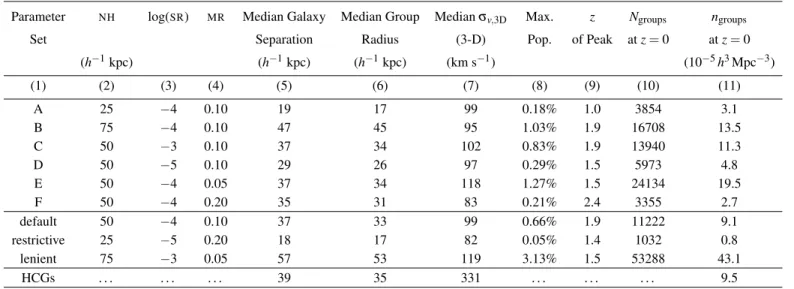
Table 1.Parameter Grid and Results

Parameter NH log(SR) MR Median Galaxy Median Group Medianσv,3D Max. z Ngroups ngroups

Set Separation Radius (3-D) Pop. of Peak atz=0 atz=0 (h−1kpc) (h−1kpc) (h−1kpc) (km s−1) (10−5h3Mpc−3) (1) (2) (3) (4) (5) (6) (7) (8) (9) (10) (11) A 25 −4 0.10 19 17 99 0.18% 1.0 3854 3.1 B 75 ₋4 0.10 47 45 95 1.03% 1.9 16708 13.5 C 50 ₋3 0.10 37 34 102 0.83% 1.9 13940 11.3 D 50 −5 0.10 29 26 97 0.29% 1.5 5973 4.8 E 50 ₋4 0.05 37 34 118 1.27% 1.5 24134 19.5 F 50 ₋4 0.20 35 31 83 0.21% 2.4 3355 2.7 default 50 ₋4 0.10 37 33 99 0.66% 1.9 11222 9.1 restrictive 25 −5 0.20 18 17 82 0.05% 1.4 1032 0.8 lenient 75 ₋3 0.05 57 53 119 3.13% 1.5 53288 43.1 HCGs . . . 39 35 331 . . . 9.5

Note. Column (1) gives the label of the observational or computational parameter set, characterized by the parameter values that were varied, as specified in columns (2), (3) and (4). Columns (2), (3), and (4) give, in order, the DBSCANalgorithm neighborhood radius; maximum mass-density ratio of galaxies in a shell surrounding a candidate group to the candidate group’s galaxies; and minimum mass-ratio of the second and third galaxies combined to the most massive galaxy in a candidate group. The remaining columns show results for HCGs or compact groups identified in the De Lucia & Blaizot (2007) catalogs produced from the Millennium Simulation, following the adoption of the selection criteria in columns (2) to (4). Column (5) gives the median galaxy-galaxy separation in a group, and column (6) the median group radius. The group radius is defined relative to the group center, taken to be the median of the positions of the identified galaxy members. The group radius is simply the greatest distance from this center to any of the member galaxies. Column (7) gives the median 3-D galaxy velocity dispersion,σv,3D≡

q

σv2,x+σv2,y+σv2,z.

The maximum fraction of galaxies that were in a compact group at the redshift given in column (9) is shown in column (8), while the redshift at which the number of compact groups was at its maximum is given in column (9). The number of compact groups at the present time is shown in column (10), and the volume number density of compact group galaxies at the present time in column (11).

1997). Such galaxies may thus be transient group members that nevertheless could have a significant effect on CG galaxy evo-lution.

4.3. Comparison to Hickson Compact Groups

We compare the properties of the CGs that we found in the De Lucia & Blaizot semi-analytical model output to those of the CGs found via the observational work of Hickson and col-laborators. In particular, we compare the space densities, the median radii, and the median 3-D galaxy velocity dispersions of the groups,σv,3D≡

q

σv2,x+σv2,y+σv2,z. The results are sum-marized in Table1.

The number of CGs identified in Hickson’s catalog can be compared to the number of CGs identified in the Millennium Simulation galaxy catalogs for specific parameter sets by mak-ing a few assumptions. While Hickson et al. (1992) identified a total of 92 groups4 with at least three accordant members withinz_≤0.14 over 67% of the sky, the median redshift of groups in the catalog isz=0.03, which suggests the catalog be-comes increasingly incomplete for larger values ofz. Further, D´ıaz-Gim´enez & Mamon (2010) found that the velocity-filtered HCG catalog is only 8% complete even atz=0.03. To this red-shift, and over 67% of the sky, there are 47 detected HCGs with accordant velocities in Hickson et al. (1992). Therefore, the 4_{Among these, a further four groups may be questionable; see D´ıaz-Gim´enez}

et al. (2012), and references therein.

expected number of CGs over 67% of the sky out toz=0.03 isNHCG=47/0.08=587.5, if we assume the Hickson cata-log is 8% complete out to this distance. On the other hand, the comoving volume toz=0.03 isV= (∆Ω/3)(DL/(1+z))3, whereDL=92.1h−1Mpc is the luminosity distance to this red-shift, and∆Ω=8π/3 is the solid angle for a 67% sky coverage. This gives a completeness-corrected expected number density of HCGs toz=0.03 ofnHCG=2.9×10−4h3Mpc−3.

The volume of a snapshot of the Millennium Simulation is

Vsnap= (500 h−1Mpc)3=1.25×108h−3 Mpc3, and there is one snapshot atz=0. Hence, if the simulation has the same volume density of groups as HCGs, we expect a total number of identified groups in the simulation to beNsim=36,250 atz=0. This number is between the number produced by set E and the “lenient” parameter set (see Table1, Column (10)). Thus, if one assumes that the space density of HCGs up toz=0.03 is representative, a more lenient set of parameters is preferred.

The median projected group separation in the Hickson et al. (1992) catalog is RHCG=39h−1 kpc. Thus, if the 3-D sep-aration is 2π/5 larger than the projected 2-D separation, then the expected 3-D HCG galaxy separation is_∼49h−1kpc. Sev-eral of the parameter sets produce median group radii that are within 20% of this value, including the “default”, C, D, E, and F parameter sets. All of these parameter sets share a common Neighborhood (NH) of 50h−1kpc, unlike all the rest of the pa-rameter sets.

0 2 4 6 8 10 12 Lookback Time (Gyr)

10−4 10−3 10−2 F raction of Galaxies in Compact Groups nh= 75h−1_kpc nh= 50h−1_kpc nh= 25h−1_kpc 0.0 0.1 0.2 0.3 0.5 Redshift1 1.5 2 3 5 10 0 2 4 6 8 10 12

Lookback Time (Gyr) 10−3 10−2 10−1 F raction of Galaxies that ha ve ev er b een in Compact Groups nh= 75h−1_kpc nh= 50h−1_kpc nh= 25h−1_kpc 0.0 0.1 0.2 0.3 0.5 Redshift1 1.5 2 3 5 10

Figure 5. Same as Figure3but varying the neighborhood parameter. Each analysis uses a maximum shell density ratio log10(SR) =−4 and a

minimum mass ratioMR=0.10. These curves are the results of varying the neighborhood parameter (NH=75h−1kpc, red circles;NH=50h−1

kpc, orange squares;NH=75h−1kpc, yellow triangles). The width of the shaded region is 50 times the Poisson uncertainty. The most restrictive

NHvalue of 25h−1kpc requires identified systems to be denser.

0 2 4 6 8 10 12

Lookback Time (Gyr) 10−4 10−3 10−2 F raction of Galaxies in Compact Groups most lenient default most restrictive 0.0 0.1 0.2 0.3 0.5 Redshift1 1.5 2 3 5 10 0 2 4 6 8 10 12

Lookback Time (Gyr) 10−3 10−2 10−1 F raction of Galaxies that ha ve ev er b een in Compact Groups most lenient default most restrictive 0.0 0.1 0.2 0.3 0.5 Redshift1 1.5 2 3 5 10

Figure 6.Same as Figure3but varying all three parameters. The “most lenient” curve (red circles) is generated using a neighborhood parameter

NH=75h−1kpc, a maximum shell density ratio log₁₀(SR) =−3, and a mass ratioMR=0.05. The “default” curve (orange squares) with values chosen to best approximate the HCG sample is the result using our “default” values ofNH=50h−1 kpc, log₁₀(SR) =−4, andMR=0.10. The “most restrictive” curve (yellow triangles) is the result usingNH=25h−1kpc, log₁₀(SR) =−5, andMR=0.20. The width of the shaded region is 50 times the Poisson uncertainty. The specific input criteria for the clustering algorithm are clearly important in determining the normalization of the curves, but their shapes in both panels are similar with compact group galaxy number peaking atz_∼1.7.

While there are parameter sets that reasonably reproduce the observed space density and sizes of HCGs, the 3-D velocity dispersion presents an issue. Hickson et al. (1992) observed a median 1-D velocity dispersion of 200 km s−1and, after con-sidering the uncertainties in the individual velocities, inferred a 3-D dispersion of σv,3D,HCG=331 km s−1. The parameter sets tested here, however, all produce significantly smaller 3-D velocity dispersions that are all<120 km s−1, and typically

.100 km s−1. We note that for groups with only 3 members, on average, the 3-D velocity dispersion we obtain is 81 km s−1, whereas for groups with 4 members or more, on average, the 3-D velocity dispersion is 159 km s−1. This shows that, even if we had setNmin= 4, we would still not be able to reconcile our results with the HCG value of 331 km s−1_.

We have performed a series of further tests to assess whether any specific modifications in our approach might result in sub-stantially different velocity dispersions, but were only able to obtain negligible changes. Specifically, we compared results from DBscan both including and excluding dwarf galaxies. We also computed 3D velocity dispersions using the biased dis-persion, unbiased disdis-persion, and gapper techniques, result-ing in median velocity dispersions atz=0 of_∼100 km s−1_,

∼125 km s−1, and_∼150 km s−1, respectively, which fall well short of the value observed for HCGs.

We postulate that this disagreement may be due to the in-herent differences between selecting observed groups based on 2-D spatial projections as opposed to actual 3-D information available in the simulations. One hypothesis is that this key

dif-Figure 7.Color-magnitude diagram of Millennium catalog galaxies at

z=0 that were in compact groups atz_∼2. Walker et al. (2013) CG galaxies are overplotted as red stars.

ference has its origin in the more restrictive selection criteria in 3-D space, resulting in more tightly bound groups than the ones in the Hickson et al. (1992) catalog.

5. Discussion

From the parameter sets used here to identify CGs, it is clear that the precise definition of CGs can have a significant impact on the resulting demographics. Nevertheless, the different pa-rameter sets do result in some broad similarities with respect to compact group populations over cosmic time. For example, all of the parameter sets tested here produce a rapid rise in the population of CGs up to a redshift ofz_∼4₋5, after which the different populations reach peaks atz_∼1₋3 and then slowly decline.

It is noteworthy that the two parameter sets that best repro-duce the properties of HCGs at redshifts ofz<0.03 (“default” and C) exhibit the peak in their populations at redshifts of

z=1.9, which mirrors the peaks in both the cosmic star for-mation rate (e.g., Madau & Dickinson 2014) and the galaxy merger rate histories (e.g., Bertone & Conselice2009). Even during this “peak” epoch of CGs, according to the results for these parameter sets, only up to_∼1% of non-dwarf galaxies reside in CGs. For these same parameter sets, only 4-5% of non-dwarf galaxies have been members of CGs at some point over cosmological time.

Despite identifying parameter sets that reproduce the sizes and population of HCGs atz<0.03, we were not able to repro-duce the median 3-D velocity dispersion of HCGs. The groups identified in the simulation have median 3-D velocity disper-sion ofσv,3D.100 km s−1, while HCGs have median 3-D dis-persion ofσv,3D,HCG∼331 km s−1. For galaxies withNmin=4,

D´ıaz-Gim´enez et al. (2012) found a higher median 1D velocity dispersion of_∼248 km s−1_{by means of mock redshift} cata-logs, which translates toσv,3D,HCG∼430 km s−1, also higher than our median_∼159 km s−1 for such CGs. We note that the value of_∼248 km s−1_{is very close to the reported value of}

∼262 and_∼237 km s−1for observed HCGs and 2MASS CGs, respectively, in D´ıaz-Gim´enez et al. (2012). This is particularly puzzling given that we adopted a relative velocity restriction of

v=_±1000 km s−1, identical to that of Hickson et al. (1992). We postulate that this discrepancy may be, in part, due to HCGs being identified based on their apparent projected spatial prox-imity, although this seems unlikely to account for a factor of

∼3 between observed and simulated groups. However, the re-cent work of Tzanavaris et al. (2019) studying the 3D evolution of individual compact groups found in simulations suggests that the velocity fields may be highly non-isotropic, and so such a possibility warrants further study. Alternatively, the discrep-ancy between simulated and observed CG velocity dispersions might instead represent a real limitation of simulations of this nature to reproduce the observed properties of galaxy systems in the low-mass group range; a mass range for which the simu-lations were not tuned.

From the results presented here, it would appear that the compact group environment is not prevalent in cosmological history. Even with the most lenient parameter set tested here (which does not fully reproduce the properties of HCGs), only

∼16% of non-dwarf galaxies have been members of a com-pact group at some point in their evolution (Figure6). A major limitation of the Millennium Simulation is its mass resolution, and the resulting exclusion of dwarf galaxies in this analysis. Given that low-mass galaxies are the dominant population at all redshifts (e.g., Binggeli et al.1988), this limitation is likely to have a significant impact on the statistics of CGs. The im-pact of excluding dwarf galaxies will be increasingly strong at higher redshifts where the relative population of dwarf galaxies approaches values of unity (see Figure2).

6. Conclusions

We investigate the prevalence of the compact group environ-ment over cosmological time using a Millennium Simulation galaxy catalog. The goals of this work are two-fold: first, to constrain the fraction of galaxies that have ever existed in this unusual environment, and second, to determine whether there is an “epoch” of CGs during cosmological history dur-ing which this environment was particularly common. To ac-complish these goals we use a number of tunable parameters to identify CGs in the simulation. The key parameters are varied over a range that is centered on “default” values that best repre-sent properties of Hickson CGs in the local Universe. The main conclusions are as follows:

1. Every set of parameters tested here produces a peak rel-ative population of CGs betweenz_∼1₋3, while both of the parameter sets that best reproduce the properties of HCGs (“C” and “default” in Table1) result in a peak relative population of CGs atz_∼1.9.

2. The fraction of non-dwarf galaxies that are members of CGs at any redshift never exceeds_∼3.2%, even for the most lenient parameter set. The best-fit parameter sets result in peak relative fractions of_.1%.

3. The fraction of non-dwarf galaxies that have ever been members of a compact group does not exceed_∼16%. The best-fit parameter sets indicate that this value is probably closer to

∼4%.

4. The exclusion of dwarf galaxies from this analysis could have a significant impact on the values presented here in the sense that the relative fractions are lower limits. Including dwarf galaxies becomes increasingly important at higher red-shifts.

5. While thez<0.03 number density and median size of our default set of CGs match those of HCGs, the 3-D velocity dis-persions of CGs are about half the measured values of HCGs. This suggests that the CGs found in the Millennium Simulation galaxy catalogs are more tightly bound than observed HCGs.

We thank the referee, G. Mamon, for detailed input that im-proved the presentation in this paper. C.D.W. thanks the Uni-versity of Virginia Small Research Grants for undergraduates for their support of this project. T.V.W is supported by the NSF through the Grote Reber Fellowship Program adminis-tered by Associated Universities, Inc./National Radio Astron-omy Observatory, the D.N. Batten Foundation Fellowship from the Jefferson Scholars Foundation, the Mars Foundation Fel-lowship from the Achievement Rewards for College Scientists Foundation, and the Virginia Space Grant Consortium. K.E.J is grateful to the David and Lucile Packard Foundation for their generous support. S.C.G. thanks the Natural Science and Engi-neering Research Council of Canada and the Ontario Early Re-searcher Award Program for support. P.T. acknowledges sup-port by NASA ADAP 14-ADAP14-0200 (PI Tzanavaris).

References

Alatalo, K., Appleton, P. N., Lisenfeld, U., et al. 2015,ApJ,812, 117

Amram, P., Mendes de Oliveira, C., Plana, H., et al. 2004,ApJL,612, L5

Barton, E., Geller, M., Ramella, M., Marzke, R. O., & da Costa, L. N. 1996, AJ,112, 871

Bertone, S., & Conselice, C. J. 2009,MNRAS,396, 2345

Binggeli, B., Sandage, A., & Tammann, G. A. 1988,ARA&A,26, 509

Birant, D., & Kut, A. 2006, Data and Knowledge Engineering, 60, 208. http://www.sciencedirect.com/science/article/pii/ S0169023X06000218

Bitsakis, T., Charmandaris, V., da Cunha, E., et al. 2011,A&A,533, A142

Bitsakis, T., Charmandaris, V., Le Floc’h, E., et al. 2010,A&A,517, A75

Blanton, M. R., Eisenstein, D., Hogg, D. W., Schlegel, D. J., & Brinkmann, J. 2005,ApJ,629, 143

Bower, R. G., Benson, A. J., Malbon, R., et al. 2006,MNRAS,370, 645

Brasseur, C. M., McConnachie, A. W., Ellison, S. L., & Patton, D. R. 2009, MNRAS,392, 1141

Cluver, M. E., Appleton, P. N., Ogle, P., et al. 2013,ApJ,765, 93

Coenda, V., Muriel, H., & Mart´ınez, H. J. 2012,A&A,543, A119

—. 2015,A&A,573, A96

Croton, D. J., Springel, V., White, S. D. M., et al. 2006,MNRAS,365, 11

De Lucia, G., & Blaizot, J. 2007,MNRAS,375, 2

Deng, X.-F., He, J.-Z., Jiang, P., et al. 2007,Astrophysics,50, 18

D´ıaz-Gim´enez, E., & Mamon, G. A. 2010,MNRAS,409, 1227

D´ıaz-Gim´enez, E., Mamon, G. A., Pacheco, M., Mendes de Oliveira, C., & Alonso, M. V. 2012,MNRAS,426, 296

D´ıaz-Gim´enez, E., & Zandivarez, A. 2015,A&A,578, A61

Ester, M., Kriegel, H., Sander, J., & Xu, X. 1996, KDD-96 Proceedings, 226. https://www.aaai.org/Papers/KDD/1996/KDD96-037.pdf Farhang, A., Khosroshahi, H. G., Mamon, G. A., Dariush, A. A., & Raouf, M.

2017,ApJ,840, 58

Freedman, W. L., Madore, B. F., Scowcroft, V., et al. 2012,ApJ,758, 24

Geha, M., Blanton, M. R., Yan, R., & Tinker, J. L. 2012,ApJ,757, 85

Geller, M. J., & Postman, M. 1983,ApJ,274, 31

Guo, Q., White, S., Li, C., & Boylan-Kolchin, M. 2010,MNRAS,404, 1111

Guo, Q., White, S., Boylan-Kolchin, M., et al. 2011,MNRAS,413, 101

—. 2013,MNRAS,435, 897

Henriques, B. M. B., White, S. D. M., Lemson, G., et al. 2012,MNRAS,421, 2904

Hickson, P. 1982,ApJ,255, 382

Hickson, P., Mendes de Oliveira, C., Huchra, J. P., & Palumbo, G. G. 1992, ApJ,399, 353

Hinshaw, G., Larson, D., Komatsu, E., et al. 2013,ApJS,208, 19

Johnson, K. E., Hibbard, J. E., Gallagher, S. C., et al. 2007,AJ,134, 1522

Karachentsev, I. D. 2005,AJ,129, 178

Lee, B. C., Allam, S. S., Tucker, D. L., et al. 2004,AJ,127, 1811

Lemson, G., & Virgo Consortium, t. 2006, ArXiv Astrophysics e-prints, astro-ph/0608019

Lenki´c, L., Tzanavaris, P., Gallagher, S. C., et al. 2016,MNRAS,459, 2948

Lisenfeld, U., Alatalo, K., Zucker, C., et al. 2017,A&A,607, A110

Madau, P., & Dickinson, M. 2014,ARA&A,52, 415

Mamon, G. A. 1986,ApJ,307, 426

—. 1992,ApJL,401, L3

Mart´ınez, H. J., Coenda, V., & Muriel, H. 2013,A&A,557, A61

McConnachie, A. W., Ellison, S. L., & Patton, D. R. 2008,MNRAS,387, 1281

McConnachie, A. W., Patton, D. R., Ellison, S. L., & Simard, L. 2009, MNRAS,395, 255

Mendes de Oliveira, C., Amram, P., Plana, H., & Balkowski, C. 2003,AJ,126, 2635

Mendes de Oliveira, C., Coelho, P., Gonz´alez, J. J., & Barbuy, B. 2005,AJ,

130, 55

Mendes de Oliveira, C., Plana, H., Amram, P., Bolte, M., & Boulesteix, J. 1998,ApJ,507, 691

Moles, M., Sulentic, J. W., & M´arquez, I. 1997,ApJL,485, L69

Mulchaey, J. S. 2000,ARA&A,38, 289

Nolthenius, R., & White, S. D. M. 1987,MNRAS,225, 505

Plana, H., Mendes de Oliveira, C., Amram, P., & Boulesteix, J. 1998,AJ,116, 2123

Pompei, E., & Iovino, A. 2012,A&A,539, A106

Proctor, R. N., Forbes, D. A., Hau, G. K. T., et al. 2004,MNRAS,349, 1381

Springel, V., White, S. D. M., Jenkins, A., et al. 2005,Nature,435, 629

Taverna, A., D´ıaz-Gim´enez, E., Zandivarez, A., Joray, F., & Kanagusuku, M. J. 2016,MNRAS,461, 1539

Torres-Flores, S., Amram, P., Mendes de Oliveira, C., et al. 2014,MNRAS,

442, 2188

Torres-Flores, S., Mendes de Oliveira, C., Amram, P., et al. 2010,A&A,521, A59

Torres-Flores, S., Mendes de Oliveira, C., de Mello, D. F., et al. 2009,A&A,

507, 723

Tzanavaris, P., Gallagher, S. C., Ali, S., et al. 2019, ApJ accepted

Tzanavaris, P., Hornschemeier, A. E., Gallagher, S. C., et al. 2010,ApJ,716, 556

Walker, L. M., Johnson, K. E., Gallagher, S. C., et al. 2012,AJ,143, 69

—. 2010,AJ,140, 1254

Walker, L. M., Butterfield, N., Johnson, K., et al. 2013,ApJ,775, 129

Wetzel, A. R., Tinker, J. L., & Conroy, C. 2012,MNRAS,424, 232