Bayesian Volterra system identification using reversible jump MCMC algorithm

Contents lists available at ScienceDirect

Signal

Processing

journal homepage: www.elsevier.com/locate/sigpro

Bayesian

Volterra

system

identification

using

reversible

jump

MCMC

algorithm

O.

Karaku

¸s

a ,∗

_,

_E.E.

_Kuruo

_˘glu

b

_,

_M.A.

_Altınkaya

a

a_{˙IzmirInstituteofTechnology(IZTECH),Electrical-ElectronicsEngineering,˙Izmir,Turkey} b_{ISTI-CNR,viaG.Moruzzi1,56124,Pisa,Italy}

a

r

t

i

c

l

e

i

n

f

o

Articlehistory:

Received24January2017 Revised1May2017 Accepted30May2017 Availableonline31May2017

Keywords:

ReversiblejumpMCMC Volterrasystemidentification Nonlinearitydegreeestimation Nonlinearchannelestimation

a

b

s

t

r

a

c

t

Volterrasystemshavehad significantsuccessinmodellingnonlinearsystemsinvariousreal-world ap-plications.However,itisgenerallyassumedthatthenonlinearitydegreeofthesystemisknown before-hand.Inthispaper,wecontributetotheliteratureonVolterrasystemidentification(VSI)withanumerical Bayesianapproachwhichidentifiesmodelcoefficientsandthenonlinearitydegreeconcurrently.Although thisnumericalBayesianmethod,namelyreversiblejumpMarkovchainMonteCarlo(RJMCMC)algorithm hasbeenused withsuccessinvariousmodelselection problems,ouruseisinanovelcontextinthe sensethatbothmemorysizeandnonlinearitydegreeareestimated.Theaforementionedstudyensures ananomalousapproachtoRJMCMCandprovidesanewunderstandingonitsflexibleusewhichenables trans-structuraltransitionsbetweendifferentclassesofmodels inadditionto transdimensional transi-tionsforwhichitisclassicallyused.Westudytheperformanceofthemethodonsyntheticallygenerated dataincludingOFDMcommunicationsoveranonlinearchannel.

© 2017ElsevierB.V.Allrightsreserved.

1. Introduction

Nonlinear modelscan befavorablecomparedtolinearonesin manyreallifephenomenawhichexhibitnonlinearcharacteristics. Ontheotherhand,usageofthesemodelsislimitedbecausethey do not have easy to implement solutions for estimating nonlin-ear model parameters. Linear-in-the-parameters nonlinear models do not share these shortcomings as far as various mathematical methods which are developed for linear models can be applied easily [1] .

Volterra models are appealing linear-in-the parameters mod-els for nonlinear modelling for several reasons. Firstly, they are flexible enoughto representvarious nonlinearsystemssince con-tinuously differentiable transfer functions can be easily approxi-matedbyVolterramodelswithTaylorseriesexpansion.Moreover, various nonlinear differential equations such as Lotka–Volterra, Schrödinger [2] , can be rewrittenas a Volterrasystem. Secondly, their inverses are also Volterratype whichprovides considerable ease in the identification of these systems [3] . This paperis in-terestedinthenonlinearitydegreeestimationofVolterramodels, withinthesystemidentification(SI)problem.

∗ _{Correspondingauthor.}

E-mailaddresses:[email protected](O. Karaku¸s),

[email protected](E.E. Kuruo˘glu),[email protected]

(M.A. Altınkaya).

TheapplicationareasofVolterramodelscoveralmostallareas ofsignalprocessing,includingspeech,image,communications, au-dio, mechanical systems, etc. To name a few: in audio, Volterra modelhasbeen usedforparametric loudspeaker system identifi-cation in [4] andfor acoustic echo cancellationin [5] .Nonlinear communicationchannelsin satellite linkshavebeen modelledas sparsethird order(cubic)Volterrasystemswhichwere estimated viaadaptive algorithms [6] . Volterrasystemmodels wereapplied also in [7] to coherent optical fiber systems outperforming the adaptivereferencemethodsonequalizingthefiberlinkchannel ef-fects.Volterrasystemswithcomplexcoefficientshavebeenusedin blindidentificationofsingle-input-single-output (SISO) communi-cationchannelswithsecond ordernonlinearity in [8] andforLTI FIRmultiple-input-multiple-output(MIMO) systemsin [9] .A gen-eralapproachintheliterature,whichissharedbythementioned applications,istoapplyVolterraSI(VSI)methodologytothe mod-els with predeterminednonlinearity degree and system memory [4–9] . Preknowledge of nonlinearity degree is an unrealistic as-sumptionformostof theseapplicationsand estimatingthe non-linearitydegreeofthenonlinearmodelisofutmostimportance.

TheBayesianapproachproposedinthispaperutilizesreversible

jump Markov chain Monte Carlo (RJMCMC) algorithm in the VSI

problemtoestimate thenonlinearitydegree, thesystemmemory andmodelcoefficientsatthesametime.Modelspaceincludes lin-ear and nonlinear models with different degrees of nonlinearity whilethegenerallyacceptedprocedureistouseRJMCMCinspaces http://dx.doi.org/10.1016/j.sigpro.2017.05.031

whichincludeonlymodelsofthesameclass thatarespaces con-taining only linear system parameters or spaces containingonly nonlinearsystem parameters of the same degree of nonlinearity. However, although RJMCMC has been used for transdimensional sampling only, the formulation in the original paper by Green [10] doesnotexcludethepotentialtoexplorespaceswhichinclude different classes of models, such aslinear and nonlinear spaces, ornonlinearspaceswithdifferentdegrees. RestructuringRJMCMC samplingstrategy fromthat definedbyGreen [10] samplingfrom thespacesofdifferentclassesofmodels,enablesapplyingRJMCMC inmorecomplicatedproblemssuchasnonlinearmodel identifica-tionornonlinearSI.

In this paper, firstly we contribute to the literature with a BayesianVSIschemeandincontrasttopreviousworks,weprovide means to estimate nonlinearity degree in addition to the mem-orysize,hencedropingtherequirementofpreknowledgeof non-linearitydegree.Thisoffers greaterflexibility inmodelling,which cancoverawidespectrumofnonlinearcharactersobservedinthe measureddata.

Secondly, we broaden the interpretation of RJMCMC transi-tionswithtrans-structuraltransitionsbeyondtrans-dimensionality by performing the original formulation in [10] between different structuralmodels.ThisalsooffersaBayesiantestprocedureto de-finethenonlinearrelationshipbetweeninputandoutputdatasets ofreallifeexperiments,suchasmechanicalsystems,optical com-municationsystems,biologicalsystems,intermsofVolterraseries expansion model structure. In our previous works,this potential wasexploitedin theestimationofpolynomial autoregressive and polynomialmovingaveragemodels [11,12] .

Furthermore, in addition to the model orders the proposed methodalsoestimatesthemodelcoefficientswithsuperior perfor-manceinapplicationsonsyntheticallygenerateddatasets includ-ing a nonlinear communication channel estimation problem. We providealsomodelselectionresultsobtainedbyAkaikeinformation criterion (AIC) and Bayesian information criterion (BIC) as bench-markstowhichour methodcanbe compared.Performance com-parisonforestimatingthemodelcoefficientsisprovidedforerror measurenormalizedmeansquareerror(NMSE)usingnonlinearleast squares(NLS)estimation.

Rest of the paper is organized as follows: background infor-mationforVolterrasystemmodels ispresentedin Section 2 .The generalRJMCMC procedureandtheproposed approach for trans-structural RJMCMC are expressed in Section 5.4 . Construction of RJMCMCforidentifyingVolterrasystemsisexaminedin Section 5 . Section 6 exhibitssimulationsetup,referencemethods,simulation resultsandperformancecomparisonstudy. Section 7 concludesthe paperwithadiscussionofexperimentalresults.

2. Volterra system models

AdiscretetimeVolterramodelwiththeoutputy(l)isgivenby [13] : y

(

l

)

=

μ

+ p m=1 q τ1=1 ... q τm= τm−1 h_τ(m_1,...)_,τm m j=1 x

(

l−

τ

j

)

(1)

where x(·) refers to the input of themodel and h_τ(m)

1,...,τm denotes

the mthorder discrete Volterra model coefficients (kernels). The nonlinearitydegreeisrepresentedbypandqspecifiesthesystem memorysize.ThisVolterramodelcanberepresentedwiththe no-tation:V(p,q).

Observing (1) , Volterra models can be represented in matrix-vector form by using the linear-in-the-parameters property:

y=Xh(p,q) (2)

wherethe

η

×1coefficientvector h (p,q)_andn×

_η

_{datamatrix X}

aregivenby: h(p,q)₌

_h(1) 1 , h( 1) 2 , ..., h( 1) q , h(12,1), h( 2) 1,2, ..., h( 2) q,q, ..., h( p) q,q,...,q

T , (3) X=

⎡

⎢

⎢

⎢

⎢

⎢

⎣

x

(

0

)

x

(

−1

)

... x

(

1 −q

)

x2

(

₀

)

_x

(

₀

)

_x

(

₋₁

)

_{... x}2

(

_{1 −q}

)

_{... x}p

(

_{1 −q}

)

x

(

1

)

x

(

0

)

... x

(

2 −q

)

x2

₍

₁

₎

_x

₍

₁

₎

_x

₍

₀

₎

_{... x}2

₍

_{2 −q}

₎

_{... x}p

₍

_{2 −q}

₎

. . . . . . . . . . . . . . . . . . . . . . . . . . . . . . x

(

n−1

)

x

(

n−2

)

... x

(

n−q

)

x2

₍

_n−1

₎

_x

₍

_n−1

₎

_x

₍

_n−2

₎

_{... x}2

₍

_n−q

₎

_{... x}p

₍

_n−q

₎

⎤

⎥

⎥

⎥

⎥

⎥

⎦

. (4)

wherenrepresentsthedatalength.ThenumberofVolterra coef-ficientshasbeendenotedby

η

andcanbecalculatedforaV(p,q) modelby:

η

=

p+q p

−1 =

(

p+q

)

! p! q! −1 . (5)

2.1. IdentificationofVolterrasystems

MethodsusedinSIproblemsprovideinformationaboutthe un-certainties which describe formulations or mathematical expres-sions aboutthe unknown systeminthecaseoflackofstructural (physical)information aboutthe system. SImethods are well es-tablishedwhen systemtobe identified islinear.Mostofreal life applications,however,havesomewhatnonlinearnature,and solu-tion fora nonlinear SI problemcan be difficult since the under-lying systemsmayhavealargenumberofpossible nonlinearities andthenumberof possiblemodelstructures mightbe veryhigh [14] .

Intheliterature,adaptivealgorithmsareverypopularinrecent years.ThesemethodsgenerallyperformVolterrasystemcoefficient estimations based on nonlinear least mean squares (NLMS), least meanpthpower(LMP),nonlinearrecursiveleastsquares(NRLS)and extendedKalmanfilters [7,15–21] .Furthermore,geneticalgorithms [22,23] ,QR decomposition [24] ,neuro-fuzzy [25] andneural net-work [26] architectureshavealsobeenusedinVSIstudies.Forall thesestudies,nonlinearitydegreeofVolterramodelisassumedto beknown.

Several studies have used Bayesian methods for system iden-tification problems [27,28] .In addition, simulated annealing (SA) [29] andtransitional Markov chainMonte Carlo(TMCMC) [14] are alsousedinSIapplicationsofnonlineardynamicalsystems. 3. RJMCMC in a new perspective

RJMCMC was introduced by Peter Green in [10] as a method fortransdimensionalsamplingbetweenspacesofdifferent dimen-sions.However, theoriginalformulationofGreenlendsitself toa much wider interpretation than justexploring spaces (“jumping” inRJMCMCjargon) ofdifferentdimensions.Thesameformulation canbeusedtoexplorespacesofdifferenttypessuchaslinearand nonlinearvariablespaces.Thisismorethan justexploring spaces

ofdifferentsizescorrespondingtothedimensionoftheparameter vector.

In the literature, RJMCMC has generally been used in linear modelidentificationproblems.Authors of [30] studied model un-certainty problemforautoregressive(AR)models byexploring the spacesfordifferentARordersviapartialandfullconditional pro-posals. RJMCMChasbeenused inautoregressiveintegratedmoving

average (ARIMA) models by Ehlers and Brooks [31] and in

frac-tionalARIMA (ARFIMA) modelsby E˘gri [32] . In [33–35] ,RJMCMC has been employed to Bayesian analysis of mixtures of distribu-tionsinGaussian,Poissonandsymmetric

α

-stable,respectively.

RJMCMC hasalsobeen employed tothe problemsof identify-ing thenonlinearmodel,threshold MA(TMA),in [36] .Inaddition, [37] employed RJMCMCinrestoringnonlinearly distortedAR sig-nals.

3.1. Generalmethodology

In [10] ,GreendefinedRJMCMCasanextendedandgeneralized versionoftheMetropolis-Hastings(M-H)algorithm [38] andstated thatitshouldthereforehavewideapplicabilityinmodel determi-nationproblems.

Assume a transition froma space x_∈X to a state y_∈X.The acceptanceratiofortheM-Halgorithmcanbedefinedby: min

1 ,

π

_π

(

₍

y

)

q

(

x

|

y

)

x

)

q

(

y

|

x

)

(6) where

π

(·) represents the target distribution andq(y|x) refers to proposaldistributionfromstatextoy.

Green’s generalization on M-Halgorithm definesthe densities

π

(x)andq(y|x)withrespecttoan arbitrarymeasureas

π

(dx)and q(dy|x).The transition kernelof the Markovchain hasbeen con-structed intwo steps,firstlydrawinganewcandidatestatey and thenacceptingthistransitionwithaprobability

α

(x,y).

Assuming that

π

(dx)q(dy|x) has a densityf with respect to a dominatingsymmetricmeasure

ξ

on_X×X,thenthedetailed bal-anceforatransitiondefinedaboveisgivenby:

α

(

x,y

)

f

(

x,y

)

=

α

(

y,x

)

f

(

y,x

)

, (7)

α

(

x,y

)

π

(

dx

)

q

(

dy

|

x

)

=

α

(

y,x

)

π

(

dy

)

q

(

dx

|

y

)

. (8) Thisequation canbesolvedasinthestandardM-Hprocedureby retaining thedetailedbalance andmaking the acceptance proba-bilitiesaslargeaspossibleifwechoose

α

(x,y)as:

α

(

x,y

)

= min

1 ,

π

(

dy

)

q

(

dx

|

y

)

π

(

dx

)

q

(

dy

|

x

)

. (9)

FollowingGreen [10] ,when thecurrentstateisxwithparameter space

θ

,a move type m is proposed withprobability Pr(x → y), whichchangesdimension,andtakesthestatetoywithparameter space

θ

∗.

Thistransitionisrequiredtosampleanauxiliaryrandomvector u fromdistributionq1(u ).Anothervector u willbegeneratedfrom distributionq2(u )toswitchbacktothestatexfromy.Inorderto guaranteethedetailedbalance,thedimensionmatchingshouldbe satisfied provided by dim

(

x

)

+dim

(

u

)

=dim

(

y

)

+dim

(

u

)

. Then, theresulting acceptanceprobability

α

(x,y)ofRJMCMCis defined by:

α

(

x,y

)

= min

1 ,

π

(

y

)

Pr

(

y→x

)

q2

(

u

)

π

(

x

)

Pr

(

x→y

)

q1

(

u

)

∂

(

y,u

)

∂

(

x,u

)

, (10) where

∂

(

y,u

)

∂

(

x,u

)

isthemagnitudeoftheJacobianwhichisneeded toaccountforchangeofvariables.

FortheconstructedRJMCMCstructuretwotypesofmovescan bedefined.Movesofthefirsttype,between-modelmoves,namely

birth and death moves, change dimension up and down

respec-tively.Theothers,within-modelmoves, whichwecallaslifemove, updatetheparameterspacebyapplyingaclassicalM-Halgorithm. 3.2.Trans-structuralRJMCMC

Theformulation ofGreen offersdeeper interpretation of tran-sition between spaces which is not limited to transdimensional sampling.Thus, exploringspaceswiththe”samedimensions” but differentstructures(saytrans-structural),orbothdifferent dimen-sions and structures, are possible by applying reversible jump mechanism of Green. Transitions from a linear model to a non-linear model may be indicated as an example for this. Trans-structuralRJMCMC revealsthe great potential of RJMCMCwithin much wider scenarios including transitions from states with the same dimensionality and different structures other than being transdimensional.

Suppose that there is a state space X=k

{

k

}

×Rnk denotes

unionofksubspaceswhichincludesmodelswithindicatork,Xk=

{

k

}

_×Rn_{k and each can be defined as different types. We mean}

withdifferenttypes,forexample,linearandnonlinearmodels or models which are driven with different probability distributions, etc.Nowsupposewehavetwosubspaces_X1 andX2 whosetypes aredifferentwherethedimensionsn1andn2 maybeequal.Target density

π

isproperonbothsubspacesanddefinedwithrespectto n1 andn2 dimensional Lebesguemeasures, respectively. The sub-spacesX1andX2haveparametersspaces

θ

1and

θ

2andbothhave properdensitiesinRn_{1 andR}n_2.

Now,defineamovetype”m”,whichperformsatransitionfrom statex∈Xtostatey∈X,withprobabilitypmandretainsthesame

statewithprobability 1−pm.Thistransitionwillbe appliedby a

transitionkernelintwostepsasindicatedintheprevioussection. Thus, detailedbalance in (8) should be provided. Transitions be-tweenmodelsofdifferentstructures, contrarytotheprevious ap-proaches,mayincludebothbirthofnewparametersanddeathof existingparameters atthesametime. Inaddition,numberof pa-rametersmaybe thesame forbothstates.These transitions pro-posetoswitchmodelswithdifferentstructures,andhencewillbe namedas switch movesintrans-structuralRJMCMCconcept.

Nevertheless, proposing vectors of variables and change-of-variablesoperationsareneededtodefineparametervectorfor can-didatestate.So,forthistype ofproblems,we defineavector u of lengthl1foratransitionfromxtoy.Also,wedefineavector u of lengthl2forthereversetransitionfromytox.Bothofthevectors u and u aresampledfromproperdensitiesq1andq2withrespect toLebesguemeasuresinRl_{1 andR}l_{2,respectively.}

Followingtheassumptionin [10] ,thegeneralformofthe trans-structuralacceptanceratioalsonecessitates definingthedensityf (theRadon–Nikodymderivative)ofasymmetricmeasure

ξ

on_X× X whichdominates the density

π

(dx)q(dy|x).Now,letthe density fbeselectedforbothdirectionsofthetransitionsas:

f

(

x,y

)

=

π

(

x

)

q1

(

u

)

pm, (11) f

(

y,x

)

=

π

(

y

)

q2

(

u

)

pmR

∂

(

y,u

)

∂

(

x,u

)

, (12)

wherep_mR isthereversemoveprobability ofm.Then, the

accep-tanceratiocanbeeasilyconstructedby (9) :

α

(

x,y

)

=min

1 ,

π

(

y

)

pmRq₂

(

u

)

π

(

x

)

pmq1

(

u

)

∂

(

y,u

)

∂

(

x,u

)

. (13)

Remark. Itcanbeclearlystatedthattheacceptanceratioof trans-structuralRJMCMCincludingtransitionsbetweenthesame

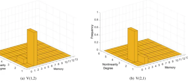
dimen-Fig.1. Toyexamplemodelestimationhistograms-(a)V(1,2) (b)V(2,1).

sionality of themodels withdifferent structures in (13) , has the sameform with the one which is derived by Green [10] for the transdimensionaltransitionsin (10) .So,Green’sformulationcanbe directlyusedwithinmuchwider implementations.Although RJM-CMChasbeen definedasa model determinationtool in transdi-mensionalcases,itwillbemoremeaningfultodefineRJMCMCas a generalmodel determination tool whether or not the parame-terspacesareofdifferentdimensions.Asfarasthesubspacesare of different structures, transitions between them require the re-versiblejump mechanism. Then, intheacceptance ratio,thecost ofthesetransitionsarefulfilledintheJacobian term,whichis re-quiredtobecalculatedduetothechangeofvariablesoperation.

InordertoseethattheuseofRJMCMCisnotlimitedto trans-dimensionalmodels,asimpleexampleisgivenasfollows.Forthis simpleexample,weconsider2modelseachhavingthesame num-berofparameters,however,oneofthemisalinearVolterramodel sayV(1,2),andtheother oneisnonlinear, sayV(2,1).The general expressionsofthemodelsfrom (1) ,aregivenbelow:

y

(

l

)

=h(₁1)x

(

l−1

)

+h(₂1)x

(

l−2

)

, (14)

y

(

l

)

=h(₁1)x

(

l−1

)

+h(₁2_,1)x2

(

l−1

)

. (15) Suppose, we are given the data, y ,observed fromone of the candidate models and there are two parameter subspaces Xk,

whichare _X1=

{

1

}

×R2 andX2=

{

2

}

×R2.Parameter subspaces willbe definedforV(1,2) asx=

(

1,h₁(1),h(₂1)

)

∈X1 andforV(2,1) asx=

(

2,h₁(1),h(₁2_,1)

)

∈X2.Also,we defineamove whichswitches subspaceswithprobabilitypmandretainsthesamesubspacewith

probability 1₋pm. When it remains in the same subspace,

RJM-CMCisgoingtoupdatemodelcoefficients.

When we need to makea transitionfromV(1,2) to V(2,1), al-though the parameter dimensionsare the same, just one of the modelcoefficients iscommon, say h₁(1).The remaining candidate coefficient,sayh(₁2_,1)_,should beproposedandh(₂1) willbesetto0. ForthereversemovefromV(2,1)toV(1,2),themechanismwillbe thesame;h(₂1) willbe proposed andh₁(2_,1) will beset to0. Coeffi-cientupdatingmechanismforthemovescanbedefinedas: Move m→_hˆ (1) 1 =h( 1) 1 ,hˆ ( 2) 1,1=u,h( 1) 2 = 0 , (16) Reverse move mR→_hˆ (1) 1 =h( 1) 1 ,hˆ ( 1) 2 =u,h( 2) 1,1= 0 , (17)

wherecoefficientswithhats onthem,e.ghˆ(₁1) representthe can-didatemodelcoefficients, variables u and u havebeenproposed fromthedensitiesq1andq2,respectivelywhichmakesJacobianof thechange-of-variablesoperationunity.

Theacceptanceratiofrom (13) appearsas:

α

(

x,y

)

=min

1 ,

π

(

x

|

y

)

pmRq₂

(

u

)

π

(

x

|

y

)

pmq1

(

u

)

∂

(

x,u

)

∂

(

x,u

)

, (18)

where

π

( _· |y ) representsthetarget distribution ofinterestgiven thedata y .

A computer simulation hasbeen performed for this problem, andRJMCMChasbeenconstructedtodecidethetruemodelgiven both input and output data ofthe Volterra models and estimate the modelcoefficientsatthe sametime. Forboth ofthe models, RJMCMCdetectstruemodelwith100%performanceafter100 real-izations.Foreachmodel,histogramsofmodelestimatesbelonging toasinglerealizationareshownin Fig. 1 .

4. On convergence and complexity of (RJ)MCMC algorithms Thecentral objectiveofMCMCsamplingistocreateaMarkov chainwithastationarydistributionequaltothetargetdistribution ortheposteriorforthemodelparameters.Ifwerunthesimulation longenough,thedistributionofoursamplesconvergestothis sta-tionary distribution. Thismakes MCMCfundamentally more out-standingthan the other sampling algorithms such as importance sampling,etc. [39] .Intheabsenceoftechniquestoselecttheright run lengtha priori,theconvergence of(RJ)MCMCrequiresonline monitoringof theestimation statisticssuch asthe meanandthe autocorrelation. The estimation of optimal run length a priori is stillanopenproblem.

There aresome advanced statisticalstudies [40–43] inthe lit-erature which propose methods for monitoring convergence. In particular, Gelman andRubin in [40,41] have proposed a way to replicate multiplechains to decide whetherornot the algorithm achieves stationarity. Brooks and Guidici in [42] generalized the method of Gelman and Rubin in a two-way analysis of variance (ANOVA) based method. In [44] , Castelloe and Zimmerman pre-sentedatwo-wayANOVAbasedapproachasin [42] butthey ex-tendedtheapproachfromunivariatetomultivariatecases.Amore recentapproach whichisa specificdistance-baseddiagnostic has been proposed by Sisson and Fan in [45] . This diagnostic is de-signedfortrans-dimensionalchainsandcoversthemodelling sce-narioslikefinite-mixtureproblemsandchangepointanalyses.

InadditiontotheconvergenceofRJMCMC,anotherkeyissueis thecomputational complexitywhichishighasintheother sam-plingalgorithms. Thecomputationalcomplexityisdirectlyrelated with their convergence and is also an open problem. However, thereare some studieswhichinvestigatethecomputational com-plexityofthesemethods.Forexample,Belloni andChernozhukov [46] statedthat computational complexityofMCMCmethods are lowerthangenericmaximumlikelihoodandextremumestimation methods when log-likelihood or quasi-likelihood are nonconcave ornonsmooth.Moreover,itisalsostatedthat computationaltime ofMCMCalgorithms ispolynomialinthedimensionofparameter space.

Regarding the convergence andcomputational issues, we will deal withthe computational gain ofRJMCMC inthis study. RJM-CMCcalculatesposteriorprobabilitiesformodelsautomatically us-ingahierarchialMCMCsamplingschemehenceavoidsvisitingall candidatemodels.Ituseslikelihoodandpriorandlearnsfromthe data in order to visit only plausible model classes. Other sam-pling methods in the literature such as Nested sampling,

transi-tionalMCMC(TMCMC),etc.needtoenumerateandobtain

posteri-orsforeachmodelclass.ThissuperiorityofRJMCMCbecomesvery clearinthepresenceofalargenumberofcandidatemodelclasses andRJMCMCprovidescomputationalgainscomparedto the sam-pling methods which perform exhaustive search on model class space.

5. Implementation of RJMCMC for Volterra systems identification

Forthepurposesofthisstudy,firstlywedefinewhatreferstoa linearspaceandanonlinearspacewithinthescopeofVSI(Please see [47] foraxiomsofalinearspace).

Proposition 5.1. ItcanbeeasilystatedthatifaVolterramodel,V(p, q)withp=1andq∈Q,namelyV(1,q),isalinearspaceSq,thenSq

satisfiesalltheaxiomsofalinearspace.

Proof. Using (1) ,aV(1,q)modelcanbeexpressedas: y

(

l

)

=

μ

+

q

i

h(_i1)x

(

l−i

)

. (19) It isseen that modeloutput n-vector y =[y

(

1

)

,y

(

2

)

,...,y

(

n

)

] is a linear combination of the input n-vector x =

[x

(

1

)

,x

(

2

)

,...,x

(

n

)

]. Thus, it can be easily shown that a V(1,q) model satisfies all the linear space axioms and is closed under bothadditionandscalarmultiplication.

Proposition 5.2. Assume thata Volterramodel,V(p, q)with p>1 is a nonlinearspace, Sp,q forp >1 and q ∈Q,thenSp,q doesnot

satisfyatleastoneoftheaxiomsoflinearspacedefinition.

Proof. Assumewedefinetwononzeroprocesses,y(l)andz(l)from aV(2,1)model,withmodelinputsx(l)andw(l),respectivelyas: y

(

l

)

=h(₁1)x

(

l−1

)

+h(₁2_,1)x2

₍

_l−1

₎

_{, (20)}

z

(

l

)

=h(₁1)w

(

l−1

)

+h(₁2_,1)w2

(

l−1

)

. (21) Letusdefinenewprocessesfromthesummationoftheoutputs andtheinputsofthesystemsabove,asr(l)andt(l),respectively:

r

(

l

)

=y

(

l

)

+z

(

l

)

, (22)

t

(

l

)

=x

(

l

)

+w

(

l

)

. (23)

Thus,VolterramodelV(p,q)tobealinearspace,Sp,q,the

pro-cessr(l)shouldbeexpressedas:

r

(

l

)

=h(₁1)t

(

l−1

)

+h(₁2_,1)t2

₍

_l−1

₎

_{. (24)}

Toshowthis,westartfromthedefinitionofr(l):

r

(

l

)

=y

(

l

)

+z

(

l

)

(25a) r

(

l

)

=h₁(1)x

(

l−1

)

+h₁(2_,1)x2

₍

_l−1

₎

_+h(1) 1 w

(

l−1

)

+h( 2) 1,1w 2

₍

_l−1

₎

_, (25b) r

(

l

)

=h(₁1)

(

x

(

l−1

)

+w

(

l−1

)

)

+h₁(2_,1)

x2

₍

_l−1

₎

_+w2

₍

_l−1

₎

_, (25c) r

(

l

)

=h(₁1)t

(

l−1

)

+2 h(₁2_,1)x

(

l−1

)

w

(

l−1

)

−2 h₁(2_,1)x

(

l−1

)

w

(

l−1

)

+h(₁2_,1)

x2

(

l−1

)

+w2

(

l−1

)

, (25d) r

(

l

)

=h(₁1)t

(

l−1

)

+h(₁2_,1)[ x

(

l−1

)

+w

(

l−1

)

] 2 −2 h₁(2_,1)x

(

l−1

)

w

(

l−1

)

, (25e) r

(

l

)

=h(₁1)t

(

l−1

)

+h(₁2_,1)t2

(

l−1

)

−2 h(₁2_,1)x

(

l−1

)

w

(

l−1

)

. (25f) The term −2h₁(2_,1)x

(

l−1

)

w

(

l−1

)

in (25f) is nonzero if h₁(2_,1) is nonzero.Thus, the sequence r(l) doesnot correspond to a V(2,1) model output and is not closed under addition. It is straightfor-wardthatthisresultcanbegeneralizedtoallVolterramodelswith nonlinearity degree, p> 1. Then, a Volterra model,V(p, q) with p> 1 is not alinear space, or equivalentlyis a nonlinearspace, Sp,q.

Corollary 5.3. Linearand nonlinearVolterra systemscanbedefined aslinear andnonlinearspaces,respectivelyunder theassumptionof thePropositions5.1and5.2.

5.1. Definingthelikelihood

TheGaussianityoftheoutputdistributionofaVolterrasystem whenthe input isnormallydistributed, isnot guaranteed dueto the polynomial operations on the input. However, in a previous study [48] ,itwasshownthatoutputdistributionofanarrowband Volterra system with white inputs is Gaussian. Following this, a Volterrasystemwhosememorytendsto infinity,generates Gaus-sian outputs due to the summation of a large number of terms followingthecentrallimittheorem.

On the other hand, the likelihood is expressed as a measure ofhowwelltheestimatedmodelrepresentstheobserveddatain BayesianSIstudies.Forthepurposesofthisstudy,we are assum-ing that the model prediction, y ˆ=[yˆ

(

1

)

,yˆ

(

2

)

,. . .,yˆ

(

n

)

], and ob-servedsystemoutput, y =[y

(

1

)

,y

(

2

)

,...,y

(

n

)

] satisfythe predic-tionerrorequation [49] :

y= ˆ y+e. (26)

In previous studies [29,49–51] , error-prediction model is as-sumed to be zeromean Gaussian. In Fig. 2 , predictionerror dis-tributions ofthreeVolterra modelswhich areused forthe simu-lationsinthisstudyare depicted.Kullback–Leibler(KL)divergence values are calculated with the fitted Gaussian distributions and ithas beenclearlyseen that predictionerrordistributions forall threeVolterramodelsare Gaussianwitha0.05significancevalue ofKLdivergence.

Thus, the likelihood function can be written simply, using a Gaussianerror-predictionmodelas:

f

(

y

|

θ

)

=

(

2

πσ

e2

)

−n/2exp

1 2

σ

2 e n t=1

(

yt−yˆ t

)

2

(27) ≈N

(

e

|

0,

σ

2 eIn

)

. (28)

where

θ

is a vector including all the parameters of

{

p,q,h (p,q)_,

σ

2

e,

σ

h2

}

, n is the length of observed data vector y .

Also e =[e

(

1

)

,e

(

2

)

,...e

(

n

)

] corresponds to the prediction error and

σ

2

Fig.2. PredictionerrorhistogramsandfittedGaussiansformodels-(a)V(1,10) (b)V(2,5) (c)V(3,3).

5.2.HierarchicalBayesmodel

Target distributionofRJMCMC,namely thejointposterior dis-tribution,f(

θ

|x ) canbedecomposedviaBayestheoremforthe pa-rametervector

θ

=

{

p,q,h (p,q)_,

_σ

2 e,

σ

h2

}

: f

(

p,q,h(p,q),

σ

2 e,

σ

h2

|

y

)

∝f

(

y

|

p,q,h( p,q)_,

_σ

2 e

)

×f

(

h(p,q)

_|

_p,q,

_σ

2 h

)

f

(

σ

h2

)

f

(

σ

e2

)

f

(

q

)

f

(

p

)

. (29) 5.3.Priorselection

Intheabsenceofrealpriorinformation,useofnoninformative priorsiscommonpractice [52] .Inthepreviousstudiesfortime se-riesmodeldeterminationproblemsusinguniformpriorformodel orderhasbeena commonchoice [11,30,31] .Inaddition,asstated in [33] ,resultsobtainedbyuniformpriors,canbeeasilyconverted tothosecorrespondingtootherpriors,usingtheidentity:

f∗

(

k,

θ

(k)

_|

_y

₎

_∝f

₍

_k,

_θ

(k)

_|

_y

₎

f∗

(

k

)

f

(

k

)

(30)

wheref∗(·|y)representstheposteriorforthepriorf∗.

So in this study, we define upper bounds pmax and qmax for

model order values p and q, respectively and assume that the model orders are independent and each model is equally likely. Therefore,uniformpriorsforthe modelmemoryq,andthe non-linearitydegreepareused:

f

(

q

)

= U

(

1 ,qmax

)

and f

(

p

)

= U

(

1 ,pmax

)

. (31) Volterra model coefficients are assumed to be normally dis-tributeda priori and forthe variances,

σ

2

e and

σ

h2, we use

con-jugatepriorswhichareinverseGamma [31] : f

(

h(p,q)

|

p,q,

σ

2 h

)

= N

(

h( p,q)

_|

_0,

_σ

2 hIη

)

, (32) f

(

σ

2 h

)

= IG

(

σ

2 h

|

α

h,

β

h

)

, (33) f

(

σ

2 e

)

= IG

(

σ

e2

|

α

e,

β

e

)

. (34)

5.4.Acceptanceratioandmoves

RJMCMC hasthreedifferent movestoperform theVSI study. These are, between-model (switch), within-model (life) and update moves.

5.4.1. Between-modelmove(Switch)

Between-model move corresponds to a move which explores thespacesofdifferentVolterramodelsateachtimeitisproposed. Models which are proposed to be switched havedifferent struc-turesandtheirspacedimensioncanbedifferentorthesame.

Theacceptanceratiofora switch movefrom(p,q)to(p,q),is definedas

α

_switch=min

{

1,r_switch

}

.Then,r_switchis:

rswitch= f

(

y

|

p,q,h(p,q)_,

σ

2 e

)

f

(

y

|

p,q,h(p,q)_,

_σ

2 e

)

× f

(

h( p,q)

_|

_p,q,

_σ

2 h

)

f

(

h(p,q)

_|

_p,q,

_σ

2 h

)

×

χ

(

u

)

χ

(

u

)

×

∂

(

h(p,q)

₎

_,u

₎

∂

(

h(p,q)_,u

₎

. (35)

where

χ

(·) willbedefinedin (45) .Modelchangesare proposed byswitchmovesandinordertoturnbacktothepreviousstate af-teraswitch moveanotherswitch moveshouldbeproposed. Con-sequently,thereversemoveoftheswitchmoveisitself.Thus,the ratiop_mR/pmin (13) isequalto1andinvisiblein (35) .

The target joint posterior distribution is proportional to the productoflikelihoodandpriorsviaBayestheorem,andhencefirst twotermsin (35) correspondtolikelihoodandpriorratios, respec-tively.Proposalratioisgivenasthethirdtermandthemagnitude oftheJacobianisshownasthefourthterm.

5.4.2. Within-modelmove(Life)

RJMCMC not only estimates model orders of a system, but alsoestimatesthe coefficientsofthemodel.Hence, theproposed and accepted coefficients in between-model moves, are updated in within-model move, namely the life move. A life move will be applied in a case when RJMCMC intends to remain at the samemodel.Acceptanceratioofthelifemoveisdefinedas

α

_life= min

{

1,r_life

}

.Hence,r_lifeis:

rlife= f

(

y

|

p,q,h(p,q)_,

σ

2 e

)

f

(

y

|

p,q,h(p,q)_,

_σ

2 e

)

× f

(

h( p,q)

_|

_p,q,

_σ

2 h

)

f

(

h(p,q)

_|

_p,q,

_σ

2 h

)

×

ψ

(

h(p,q)

|

p,q,h(p,q)

)

ψ

(

h(p,q)

|

_p,q,h(p,q)

)

. (36)

Updatingmodelcoefficientsincludesproposingfromthe distri-bution

ψ

(·):

_h(p,q)_∼

_ψ

₍

_h(p,q)

_|

_p,q,h(p,q)

₎

₍₃₇₎

=N

(

h(p,q)

_|

_μ

_n,

−1

n

)

, (38)

where

μ

n=

σ

e−2

−n1X Ty ,and

n=

σ

e−2X TX +

σ

h−2I η.

5.4.3. Updatemove-updatingvariances

RJMCMCsetup for VSIproblemincludes an errorterm within mostofthedefinitions.The varianceofthiserrorterm,

σ

2

e is

dis-tributionfor

σ

2 e isconstructedasderivedin [30] : f

(

σ

2 e

|

y,p,q,h(p,q)

)

∝f

(

y

|

p,q,h(p,q),

σ

e2

)

f

(

σ

e2

)

(39) ≈N

(

e

|

0,

σ

2 eIn

)

IG

(

σ

e2

|

α

e,

β

e

)

(40) =IG

(

σ

2 e

|

α

en,

β

en

)

, (41) where

α

en=

α

e+1 2nand

β

en=

β

e+ 1 2e T_{e .} Similarly,thefullconditional distributionfor

σ

2

h isobtainedas [30] : f

(

σ

2 h

|

y,p,q,h( p,q)

₎

_∝f

₍

_h(p,q)

_|

_σ

2 h

)

f

(

σ

2 h

)

(42) ≈N

(

σ

2 h

|

0,

σ

2 hIη

)

IG

(

σ

2 h

|

α

h,

β

h

)

(43) =IG

(

σ

2 h

|

α

hn,

β

hn

)

, (44) where

α

_hn=

α

_h+1 2

η

and

β

hn=

β

h+ 1 2

(

h ( p,q)

₎

T_h (p,q) _and

_η

_has beendefinedin (5) . 5.5. Proposingcandidates

EachRJMCMCiteration requiresto selectoneofthe switch or life move firstly withprobabilities Pswitch andPlife.Uniform prior is selected for all candidate switchable models (with probability P_switch/

ρ

for

ρ

possiblemodels).

Allcandidatecoefficientsshouldbeproposedfromtheproposal distribution.Forinstance,incaseofaswitchmove corresponding toamodelchangefromp=1top=2whenq=2,

λ

=5−2=3 candidatecoefficients areneededto be proposed.The

λ

-vector u has beenproposed froma multivariate Gaussian distribution and

χ

(u )isassumedtobe:

χ

(

u

)

= N

0,

_σ

2 h

ζ

E[

|

y

|

]

I_λ

, (45)

whereE[|y |]istheexpectedvalueoftheabsolutevalueofthedata vector y and

ζ

isthemodulationconstant.

The variance ofthe joint distribution is chosen to depend on thedata.Casesinthisstudyincludeadditionalnoiseprocessesto theI/OdatasetsoftheVolterrasystem.Inordertotakeadditional noise intoconsideration inthe proposals,E[|y |]has beenusedin

χ

(·).Furthermore,whenamodulationhasbeenperformedinthe system,thisinformationisalsoutilizedintheproposaldistribution

χ

(_·)viaparameter

ζ

.Thisdataandmodulationdependentadhoc choiceaddsvarietyforcandidateproposalsaccordingtothegiven data.Forsyntheticallygenerateddatacase,i.e.nomodulationcase (Simulation 1)

ζ

is assumedto be 1 andfor M-ary modulations (Simulation2)

ζ

isequaltolog2(M).

Moreover,theproposaldistributionforcandidatecoefficientsis selected in a way that the candidates will be independent from recentcoefficients.Consequently,thechangeofvariablesoperation isaccomplishedthroughanidentityfunctionandthustheJacobian equalstounity.

6. Experimental analysis

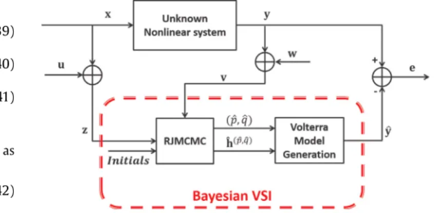
In this section, we study the performance of the proposed VSI algorithmexperimentally.The block diagram ofthe proposed Bayesian VSI procedure has been shown in Fig. 3 for a system whoseinputandoutputaredefinedwiththevectors x and y , re-spectively.Moreover,additive noisesequencesfortheseinput and outputvectorsare u and w ,respectively.

Estimated model order parameter pair

(

p,q

)

and resulting model coefficient vector h (p,q) _{will be used to generate one-step} aheadpredictionoftheoutputdata,y ,byusingtheVolterramodel

Fig.3. TheproposedmethodVSIblockdiagram.

expressionin (1) .In Table 1 RJMCMCimplementationstepsforVSI studyhasbeendepictedbriefly.

6.1. Simulation1:syntheticallygenerateddata

Theproposedmethodhasbeenemployedinsynthetically gen-erated data sets for this simulation scenario. 3 Volterra models which are V(1, 10), V(2, 5) and V(3, 3) have been implemented modelcoefficients of which havebeen depicted in Table 2 . Each modelhasbeengivenaninputsequencewhichisaGaussian pro-cessofmean 0and variance 1andoutputs for each modelhave been collected. Each dataset has a length of 1,000samples and meanvalue,

μ

,ischosen as0forsimplicity.Fourcaseshavebeen employedinordertoshowtheperformanceoftheproposed meth-odsunderdifferentconditions(See Table 3 ).

Initial values for hyperparameters of prior distribution of

σ

2 e,

areselectedas

α

e=1and

β

e=1andthosefor

σ

_h2,areselectedas

α

h=35and

β

h=2.Theinitial nonlinearitydegreep0 andsystem memoryq0aresetto1andupperboundspmaxandqmaxaresetto

5and12,respectively. h (p₀,q₀)_{issampledfromtheprior}

distribu-tionin (32) .Move probabilities,Pswitch andPlife areboth selected as0.5.Calculated signal-to-noise ratio(SNR) valuesindecibelsfor eachmodelandeachcasehasbeendepictedin Table 2 .

ModelorderestimationperformanceofRJMCMCiscomparedto twocommonlyused modelorderselection methods AICandBIC. Theequationsforthesearegivenbelow:

AIC = 2 N+nlog

(

RSS /n

)

, (46)

BIC = log

(

n

)

N+nlog

(

RSS /n

)

, (47)

whereN is number ofparameters for the model,n refers to the data length and RSS corresponds to the residual sum of squares whichiscalculatedas:

RSS =yT_y−yT_X

₍

_XT_X

₎

−1_XT_{y. (48)}

AICrewardsgoodnessoffitbutpenalizesthenumberofestimated parametersof themodel.BICis moreinformedthen AICandthe penaltytermofBICismorestringentthanthepenaltytermofAIC. Consequently,BICtendstofavorsmallermodelsthanAIC.

A similar penalization is also present in RJMCMC whenever modeltriestoaddredundantvariables.Forexample,increasing or-derby oneandsettingtheadditionalcoefficient tozerodoesnot changethelikelihood, buttheprior takesalower value than be-fore,yielding aposterior probability lowerthan theprevious one [53] .

Table 4 showsthemodelselectionperformanceofRJMCMCand referencemethodsAICandBIC after100 simulationsfor100

dif-Table1

RJMCMCAlgorithmforVSI.

Table2

DetailsforVolterramodelsinsimulation1.

V(p,q) h(p,q)_=[h(1)_{, h}(2)_{, ..., h}(p)_]T _{CalculatedSNR(dB)values}a V(1,10) h(1)_{=[0.5,0.5,0.5,0.5,0.5,0.5,0.5,0.5,0.5,0.5] 14.13/22.62/10.42/14.19} V(2,5) h(1)_{=[0.7,0,0.2,0,−0.7] 13.52/22.24/10.42/13.58} h(2)_{=[0,0.1,0,0,−0.25,0.15,0,0.42,0.02,0,0.7,0,−0.31,0,0.28]} V(3,3) h(1)_{=[−0.06,0.2331,−1.3619] 17.69/26.33/10.44/17.77} h(2)_{=[0,0.7,0,0.3,−0.25,0.15]} h(3)_{=[0.5,0,0,−0.44,0.15,−0.25,0,−0.37,0,0.58]}

a _{CalculatedSNRvaluesindBsarepresentedforCase2/Case3/Case4-Input/Case4-Output,respectively.}

Table3

Casesforsimulation1. Details

Case1 BothI/Oarenoisefree

Case2 OutputiscorruptedbyawhiteGaussian noiseprocessofmean0andvariance0.1

Case3 OutputiscorruptedbyacoloredGaussiannoiseprocess. ThewhitenoiseinCase2isfilteredbyanFIRfilter, andtheoutputofthefilterisusedtocorrupttheoutput. Case4 BothI/OarecorruptedbywhiteGaussian

noiseprocessesofmean0andvariance0.1

ferentdatasetsfrom3differentVolterramodels.IneachRJMCMC realizationthemostvisitedmodelafterburn-inperiodistakenas thedetectedmodel.Examiningthecorrectlydetectedmodelorder percentagesinthe Table 4 ,AICalwaysfallsshortofselectingtrue modelorderpairascomparedtothatofRJMCMCandBIC.RJMCMC andBIC achieve generally the same percentages, however, when themodelisnonlinear(V(2,5)andV(3,3)),RJMCMCperforms bet-ter.Forcase4,performance of RJMCMCis superiorfornonlinear models and its percentage of detection is atleast 89%, however BICachievesatmost13%forthesamemodels.

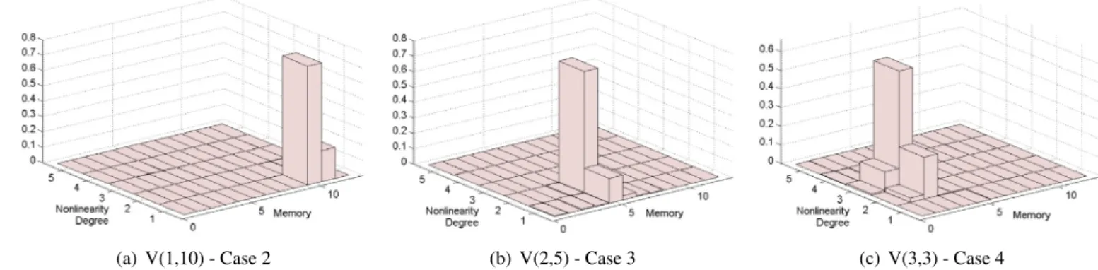
Fig. 4 shows the joint posterior density of the model orders, p and q for the simulated models and randomly selected cases ina single example realization. It has been stated that RJMCMC

Table4

Percentageofdetectingcorrectmodelorders.

Case1 Case2 Case3 Case4

V(1,10) RJMCMC 100% 100% 100% 100% AIC 99% 84% 89% 76% BIC 100% 100% 100% 100% V(2,5) RJMCMC 100% 99% 100% 93% AIC 93% 68% 85% 0% BIC 99% 100% 100% 11% V(3,3) RJMCMC 100% 100% 100% 89% AIC 98% 83% 93% 0% BIC 99% 100% 100% 13%

estimates true model order higher than 50% for each example realizations.

Nextwe comparethesuccessofRJMCMCinestimatingmodel coefficients with NLS estimate which is obtained via the aug-mented datamatrix X .NLShas beengiventhecorrectmodel or-dersp,andqandperformsestimationformodelcoefficientsas: ˆ

hNLS=

(

XTX

)

−1XTy, (49)

wherevector y isoutputdataand X isthedatamatrixwhichhas theformdefinedin (4) .

The performance comparison study has been made on the modelcoefficientestimationofRJMCMCandNLSmethodsinterms

Fig.4. Thejointposteriordensityofthemodelordersof(a)-V(1,10),(b)-V(2,5),(c)-V(3,3).

Fig.5. Estimatedoutputhistogramsforallcasesandallmodelsinsimulation1viaRJMCMC.Realdatameanvaluesareplottedusingverticallineswith“o” markers.Each rowshowstheresultsforsimulatedmodelsandeachcolumnshowstheresultsforsimulationcases.

Table5

PerformancecomparisonofmodelcoefficientestimationintermsofNMSE.

Case1 Case2 Case3 Case4

V(1,10) RJMCMC 5.89E−07 2.36E−06 2.47E−06 1.43E−03 InformedNLS 2.42E−09 8.46E−07 7.86E−07 1.26E−03 V(2,5) RJMCMC 6.76E−08 2.06E−05 1.12E−07 1.42E−03 InformedNLS 8.42E−09 1.93E−05 7.73E−08 1.32E−03 V(3,3) RJMCMC 1.69E−04 1.84E−04 1.74E−04 6.07E−03 InformedNLS 6.76E−08 2.28E−07 3.90E−08 3.46E−03

oferrormeasure,NMSE,whichcanbedefinedby: NMSE =1

η

η i=1

(

hi−hi

)

2 h 2 2 , (50)

where h isthe

η−

vectorofmodelcoefficients,h isitsestimateand h 2 isthel2-normof h .

Model coefficient estimationperformance forall three models andallfourcasesareshownin Table 5 .ExaminingNMSEvaluesin Table 5 showsthatNLSestimationachieveslowererrorvaluesthan RJMCMC for all the cases. Notwithstanding, RJMCMCshows very closeperformancetotheNLSmethod.NotethattheNMSEfigures ofNLSarehypotheticalsincetheyarebasedonunavailableperfect modelorderestimates.Consequently,modelcoefficientestimation

performanceof RJMCMCappearsremarkablebecauseit estimates modelordersandcoefficientsatthesametime.

Fig. 5 showsestimated output datahistogram foreach of the twelvesyntheticallygeneratedVolterramodeldata.Observingthe subplots in Fig. 5 depicts that realdata meansstand in thehigh probability ranges of estimated data distributions and this re-veals the good model estimation performance of the proposed method.

Asstatedintheprevious sections,RJMCMCisalearning algo-rithm which avoids performing exhaustive searches, instead per-formsa modelsearch by usingthe likelihood,the priorsandthe datatovisitonlyplausiblemodels.In Table 6 ,calculationson com-putationalgainofRJMCMCforsimulation1hasbeendepicted. Ex-amining ”Total” columns showsthat higherthan 50% ofthe can-didate models (in all the cases these are wrong models) have not been visitedand RJMCMCdecides ”truemodel” only visiting a smallsubset of themodel space.Analysingthe ”Avg.” columns shows that the search subset is smaller than the total amount and we can state that RJMCMC decides ”true model” by exam-ining at mostonly one fifth of the model space (at most 12–13 models over 60possible models). Thus, this exhibitsthe compu-tational gainsof RJMCMC comparedwith the other model selec-tion methods AIC, BIC or the sampling algorithms Nested sam-pling,TMCMC,etc.whereallperformexhaustivesearchsonmodel space.

Table6

RJMCMCcomputationalgain.

Case1 Case2 Case3 Case4

Totala _Avg.b _Totala _Avg.b _Totala _Avg.b _Totala _Avg.b

V(1,10) 16 12.37 18 12.65 16 12.31 17 12.51

V(2,5) 20 10.22 15 9.08 20 10.98 20 13.3

V(3,3) 18 8.11 20 8.06 19 8.5 26 9.79

EachRJMCMCrunhasperformed30,000iterations,andnumberofvisitedVolterramodelshasbeenrecordedforeach run.

Modelspaceincludes60Volterramodels.

a_{NumbersatTotalcellsrepresentthetotalnumberofdistinctVolterramodelsvisitedafter100RJMCMCruns.} b_{NumbersatAvg.cellsrefertotheaveragenumberofVolterramodelsvisitedatasinglerunafter100RJMCMC}

runs.

6.2.Simulation2:nonlinearchannelestimation

Incommunicationsystems,duetohigh-poweramplifiersatthe transmittersideandfilteringoperationsatthereceiverside, non-linear input-output characteristics are frequently observed. Most of these nonlinearities can be approximated via Volterra series. Anonlinearcommunicationchannel isexpressedintermsof dis-cretetimebasebandVolterramodelwithsymmetriccoefficientsas [16,54] : y

(

l

)

= p+1 2 ν=1 q m1=1 ... q m2ν−1= m2ν−2 h(m21ν,−...1,m)2ν−1 ν i=1 x

(

l−mi

)

× 2ν−1 j= ν+1 x∗

(

l−mj

)

. (51)

where x(l) and y(l) represent the complex input and output en-velopesof the system, pis the nonlinearity degree and q is the memoryofthechannel.The(2

ν

₋1)st-orderVolterracoefficientis referredtoash_m(2ν−1)

1,...,m2ν−1.Moreover,ithasbeenstatedin [55] that

powers of even-ordered terms do not contribute to the output. Thus,onlyodd-orderedterms(p=1,3,...)aretakenintoaccount forbasebandVolterrarepresentationin (51) .

Manymoderncommunicationsystemssuchasasymmetric dig-italsubscriberline (ADSL)modems, digitalvideo broadcastingand recentmobile communication systems in4G, utilize OFDM tech-nique.However,duetoitshighpeak-to-averagepowerratio,OFDM is very vulnerable to nonlinearities [54] . For these reasons, an OFDM communicationsystemwhich transmits through a nonlin-earcommunicationchannelhasbeenimplemented.Theproposed BayesianVSImodelhasbeenemployed toestimatethisnonlinear channelintermsofVolterraseries.

We assume that abaseband Volterramodelin (51) represents theunknownnonlinearcommunicationchannelwithnonlinearity degreeof3andmemoryof2.Uniformlydistributedmessagebits have been modulated via M-QAM modulations for M=4,16,64. (4QAMisthesameasquadraturephase-shiftkeying(QPSK)andwill be notated asQPSK forthe rest ofthe text.)Modulated symbols have been sent through an OFDM system with 512 sub-carriers. Resultingsymbolshavebeenparallel-to-serialconvertedand trans-mittedthroughthenonlinearchannel.AfteraddingwhiteGaussian noise, the transmitted corrupted signal has been received at re-ceiver.

Pilot messages have been employed in order to apply a VSI procedure.Hence, bothpilot OFDM output andthe corrupted re-ceivedsignalareknownatthereceiverasinputandoutputofthe unknown system, respectively. RJMCMC uses these I/O signalsto identifythe unknown nonlinear channel. Consequently, proposed methodestimatesthenonlinearitydegree,thesystemmemoryand thecorrespondingchannelcoefficients.Initialvalueshavebeen

se-Fig.6. PercentageofcorrectlyestimatedmodelorderviaRJMCMCforvaryingSNR. (Nonlinearchannel,V(3,2)).

lectedas

α

e=1,

β

e=1,

α

h=35and

β

h=2.Theinitialsystem

or-dersare q0=1and p0=1.The upperbounds are qmax=12 and

pmax=5. RJMCMC takes all the model orders into account

be-tween p=1 and p=5 whether it is odd or even and decides the true Volterra model for the nonlinear channel. For additive noiseprocesses,symbol-to-noiseratio(Es/N0)valuesbetween−5dB and 25 dB have been used in order to measure performance of the proposed method under different noisy conditions. A single RJMCMC run have performed 20,000 iterations and simulations havebeenrepeatedfor100MonteCarlorunsandresultsare pre-sentedasaverageoftheserepetitionsinorderto removerandom realization effects. Simulated channel coefficients have been se-lected ash1=[0.5, 0.3]andh3=[−0.7, −0.2, 0.34, −0.27] forlinearandcubictermsofthebasebandVolterramodelin (51) , respectively.

Percentages of correctly estimated model orders for varying SNRvaluesareshownin Fig. 6 .Examining Fig. 6 itcanbe clearly statedthat, RJMCMCcorrectlyestimatesthe truenonlinear chan-nel, V(3,2), with a remarkableperformance by obtaining atleast 99%after100RJMCMCrunsforall themodulationsatSNRvalues higherthan0dB.Below0dB,truechannel iscorrectlyestimated atleast85%timesoftherepetitions.

Fig. 7 depicts the NMSE values in logarithmic scale between estimated channel coefficients and true coefficients. Examining Fig. 7 shows that for all modulation schemes and noise scales theproposed methodachievesvery closeresultstoInformed NLS method.ForlowerSNR values,estimationperformancesare lower as expectedand NMSE values are around 10−3 _{for SNR of 0 dB,} when NMSE values for all the cases are below 10−5 _{at SNR of} 25dB.