Energy Efficient Temperature Control for Peak Power Reduction in
Building Cooling Systems
Chang-Jin Boo
1, Jeong-Hyuk Kim
1, Ho-Chan Kim
1, Min-Jae Kang
2and Kwang Y. Lee
31
Department of Electrical Engineering, Jeju National University, Korea,
2
Department of Electronic Engineering, Jeju National University, Korea,
3
Department of Electrical and Computer Engineering, Baylor University, USA,
{boo1004, ggum21c, hckim}@jejunu.ac.kr, [email protected],
[email protected]
Abstract
In this paper, an energy efficient temperature control algorithm for peak power reduction in cooling systems of a large glass-covered building is proposed using control horizon method. A control horizon switching method and linear programming algorithm is used for optimal control, and a time-of-use (TOU) electricity rate is included to calculate the energy costs. Simulation results show that the reductions of energy cost and peak power can be obtained using proposed algorithms.
Keywords: Energy saving, optimal control, linear programming, peak power reduction, control horizon, building indoor temperature control
1. Introduction
Temperature control in buildings has received much less attention from control engineering communities than other application fields like aerospace, petro-chemical, electronic or automotive industry. One of the reasons is that the effects of poor control cannot be easily noticed in temperature control of buildings. Therefore, buildings waste large amounts of energy due to poor control performance and have a potential for considerable savings by improving the control [1].
In order to reduce peak power, utilities provide price incentives for use of electricity during low demand or off-peak periods. Demand response (DR) control in building energy systems is an approach to give incentives to customers to change their electric usage pattern from their regular practice, in response to the time -varying price of electricity. The use of building thermal storage has been recognized as an important mean to reduce the peak demand for decades [2, 3].
Model-based control algorithms are desirable for both building designers and operators in that they can be simulated and tested even before a building is actually built. Moreover, an effective control system for one building is relatively easier to be adjusted and applied to another. Nowadays, time-of-use (TOU) electricity rates have been implemented on most smart grids for demand response. Significant potential savings have been shown by previous studies in model-based demand shifting and limiting control, through various simulations and field tests [4, 5].
Model Predictive Control (MPC) has several features that make it suitable for the problems encountered in intermittently heated buildings [6]. The MPC optimizes not only the comfort but also an energy usage. As heating systems generally consume energy to provide thermal comfort, MPC makes a trade-off between energy savings and thermal comfort. The MPC recently has been successfully applied on real occupied buildings [7, 8].
The paper focuses on the application of MPC to cooling systems that is charged on TOU rates. An MPC approach with linear programming (LP) algorithm is selected to model and simulate the cooling systems for peak power reduction. An MPC strategy is selected, because its periodic re-optimization characteristic provides stability during external disturbances. The periodic re-optimization also compensates for inaccurate or simplified system models.
2. One Zone Building Modeling
In order to formulate the reduced model of the building, models are represented in state-space by a set of first order differential equations. Moreover, the used MPC algorithm also requires the model of the system in the state -space representation. Low-order building models used for control purpose are most often derived from linear network representations with lumped parameters [1].
By covering a space with a glass skin, particular attention should be paid to the effects on indoor climate. In the hot season, the solar radiation both absor bed and transmitted by the glass sheet can overheat the underneath environment to temperature s which are incompatible with an acceptable thermal environment. The indoor climate depends on the external climate conditions, the building shape, type of buildin g materials (insulation, thermal mass), internal heat gains (people, lighting) and building systems like heating, cooling and ventilation. To get more feeling for different design parameters, the energy balance of a large glass-covered space will be discussed [9].
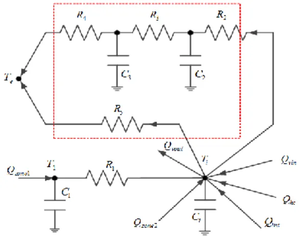
The energy balance network of one zone building can also be shown in a simplified thermal network in Figure 1. The resistances R in this network are equal to the thermal resistances of the building envelope and the capacitors C are equal to the thermal capacity [10].
Figure 1.Simplified thermal network of one zone building
For the operating temperature range of the one zone building, the model is considered to be linear. In order to find the input -output equations for building from Figure 1, the superposition theorem for electrical circuits is applied . For each mesh,
different energy flows can be analyzed and written in a so-called ordinary differential equation. Thus, the following equation is obtained:
1 1 1 1 2 2 3 2 2 3 2 2 3 2 2 3 i zone f i i i i T T dT C Q d dt R T T T T dT C dt R R T T T T dT C dt R R (1) 1 2 1 5 (1 ) ( ) i i i i e i hc ins zone f e i i dT T T T T T T C Q Q Q d mc T T dt R R R (2)
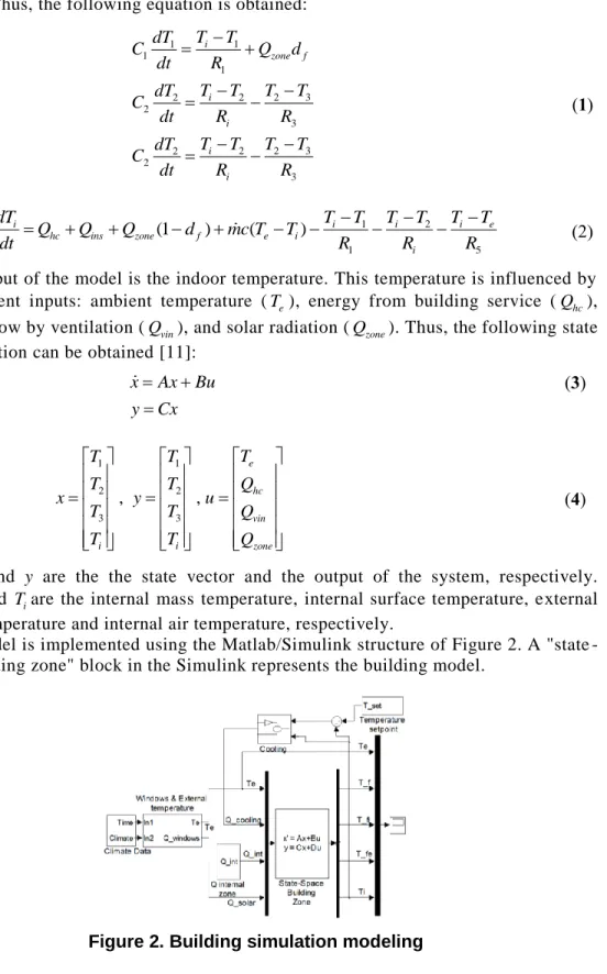
The output of the model is the indoor temperature. This temperature is influenced by four different inputs: ambient temperature (Te), energy from building service (Qhc), energy inflow by ventilation (Qvin), and solar radiation (Qzone). Thus, the following state space equation can be obtained [11]:
x Ax Bu y Cx (3) 1 1 2 2 3 3 , , e hc vin i i zone T T T T T Q x y u T T Q T T Q (4)
where x and y are the the state vector and the output of the system, respectively.
1, 2, 3
T T T and Tiare the internal mass temperature, internal surface temperature, external
surface temperature and internal air temperature, respectively.
The model is implemented using the Matlab/Simulink structure of Figure 2. A "state -space building zone" block in the Simulink represents the building model.
3. Energy Efficient Temperature Control for Peak Power Reduction
3.1. Minimal Energy Cost Function in Cooling Systems
Since the purpose is to ensure thermal comfort with minimal energy consumption, the MPC cost function must reflect these performances in a mathematical formulation. Thus, the proposed cost function minimizes energy consumption, subject to constraints on indoor temperature, which should be higher or equal to the lower limit of the comfort range. This formulation being linear, allows the use of the LP method for solving the optimization problem. In this paper, we used the following objective function to represent the daytime electricity expense, which is a combination of a TOU tariff and a critical peak (CP) charge.
max 1 min ( ) ( ) N cp k J u k p c k p C
(5)where the variable ( )u k need to be solved by the optimization algorithm over the control horizon (H) at the time k, p is the power consumption, and c k( ) accounts for the TOU electricity rates in the k-th switching interval. pmax is the maximum value of { ( )u k p} for 1 k N and Ccpis the CP charge which are applicable in on-peak and mid-peak times. If a control horizon (H) of daytime is divided into 15 min switching intervals, then, N = 36 is the total number of time steps per daytime.
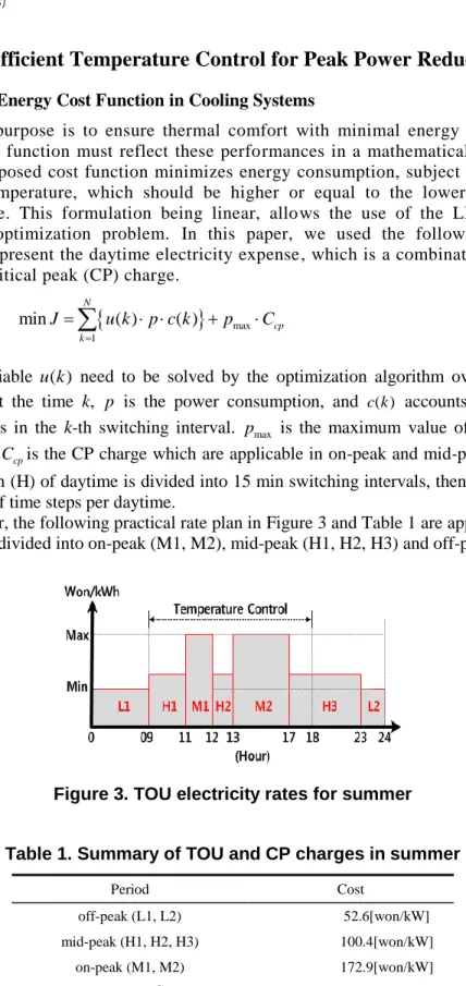
In this paper, the following practical rate plan in Figure 3 and Table 1 are applied, in which time period is divided into on-peak (M1, M2), mid-peak (H1, H2, H3) and off-peak (L1, L2).
Figure 3. TOU electricity rates for summer
Table 1. Summary of TOU and CP charges in summer
Period Cost
off-peak (L1, L2) 52.6[won/kW] mid-peak (H1, H2, H3) 100.4[won/kW] on-peak (M1, M2) 172.9[won/kW] CP charge (Ccp) 350.0[won/kW]
Equation (5) is an optimization problem. We can transfer the maximum term into a linear term so that it can be readily solved by linear programming routine. Additional inequality constraints can also be directly imposed on the zone temperature to reg ulate them within a range with respect to time. This implies that constraints need to be added to the cost function (5):
low t high
T T T (6)
The current temperature-based control model is also defined as a discrete -time model, which is based on the state space model in (3). The indoor temperature at the t -th switching interval is defined as [12]
1 0 1 ( ) ( ) ( ) t t k T T TEMPIN k TEMPOUT k u k
(7)where T0 is the initial temperature and t1, ,N. The upper level limit is used as the initial level, i.e., T0Thigh. When the cooling system is shut off, TEMPIN k( ) is the influenced temperature by four different input sources. TEMPOUT k( ) is the influenced temperature by cooling systems over the k-th switching interval. The two levels of the cooling systems are the lower and upper bound of the defined thermal comfort region (Tlow26°C and Thigh 28 °C).
There still exists potential to reduce the peak load, and then save money on a TOU pricing, by wisely pre-designing the cooling set-point schedules. However, performing an efficient strategy requires significant amount of knowledge and efforts from building operators, and it is hard to generally evaluate how good a strategy is unless a particular building is targeted.
The On/Off temperature control algorithm of the cooling systems is based on the revised switching levels, and it is defined as
0 when ( ) 1 when t low t high T T u k T T (8)
3.2. MPC Control Algorithm using Linear Programming
The MPC control strategy can be explained further with Figure 4, which shows the result of a hypothetical controller that controls the level of one zone building. The control model in Figure 4 uses 15 min switching intervals, and a control horizon (H) of 9h. The process of the MPC controller in Figure 4 can be described as follows: At the current time (11h) the controller samples the current indoor temperature, applies all the constraints, and predicts the future statuses of the cooling system that will optimize cost over the next 7 h. The figure shows the indoor temperature deviation and the statuses of control inputs over 24 h. It shows that the current time is 11h which means that the inputs and output prior to 11h are historical and the inputs and output after 11h are the future predicted values. Note that the MPC sampling intervals are chosen to coincide with the switching intervals of the cooling systems.
However, once the predicted inputs are calculated only the first predicted input is implemented and the rest of the predicted inputs are discarded. After the first predicted input is implemented the entire optimization process is repe ated. This means that the cooling system is switched on for 15 min, and when the 15 min interval lapses the level
of the reservoir is sampled again, the constraints are re -applied and the future statuses of the cooling system over the next.
Figure 4. Control horizon switching strategy
The LP optimization problem is solved with the Matlab function (linprog). The
linprog functions can be used to solve the following minimization problem:
max 1 minimize : ( ) ( ) subjec to : N cp k low t high J u k p c k p C T T T
where u represents the vector of variables, p and c are vectors of known coefficients and Tt is the function of variables u.
4. Computer Simulations
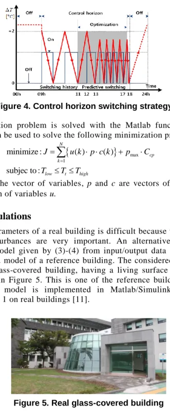
Identifying the parameters of a real building is difficult because the inputs cannot be varied and the disturbances are very important. An alternative is to identify the parameters of the model given by (3)-(4) from input/output data records obtained by simulating a detailed model of a reference building. The considered reference building is a typical large glass-covered building, having a living surface of 54.85[m2] and a volume of 253[m3] in Figure 5. This is one of the reference buildings in Jeju Island, Korea. Its detailed model is implemented in Matlab/Simulink toolbox and was summarized in Table 1 on real buildings [11].
Table 2. Building Parameters
Parameters Value Volume zone 253[m3]
Ventilation 1[h] Façade surface 49[m2]
Façade heat resistance 0.11[ m2K/W] Floor and internal walls surface 122[m2]
Window surface 44[m2]
Window heat resistance 3.6[ m3K/W]
This paper simulates and compares the following two control algorithms. (1) On/Off control algorithm.
(2) MPC control algorithm with linear programming (LP) ( 0u k( ) 1, k1, ,N).
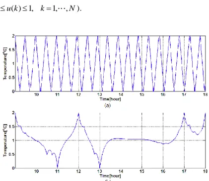
Figure 6. Comparisons of internal air temperature: (a) On/off, (b) MPC with LP
Figure 7. Comparisons of peak power with On/off, MPC without CP charge, and MPC with CP charge
Figures 6 and 7 show the simulation results of two control algorithms. In Figure 6, we see that the two temperatures in the cooling systems are operated in the lower and upper bound of the defined thermal comfort region (Tlow 26°C and Thigh 28 °C).
Furthermore, the proposed MPC with LP method is more effective than on/off method, because the temperature is slowly changed. Figure 7 shows that when we use the objective function which is a combination of a TOU tariff and a critical peak (CP) charge, the peak level of power with MPC control methods are lower than the on/off control method, i.e., 1.6kW vs. 2.8kW. This is caused by the moving control horizon (H) of the MPC control method, which means that after each implemented control step the MPC algorithm is optimizing more into the next cycle. Thus the proposed temperature profile is good because it meets the comfort conditions and save maximum energy. Figure 6 shows that the MPC control method results in a TOU saving of 4.57% and a CP saving of 42.85% per daytime.
5. Conclusion
This paper proposed a building indoor temperature control algorithm for saving energy cost and reducing peak power in cooling systems using the MPC control method. In the MPC algorithm, the optimization problem with constr aints is transformed into a linear programming and solved in each time step. Future works include the implementation of the MPC controller for a practical building plant when the simulation is mature.
Acknowledgements
This research was financially supported by the Ministry of Knowledge Economy(MKE), Korea Institute for Advancement of Technology(KIAT) through the Inter-ER Cooperation Projects.
References
[1] I. Hazyuk, C. Ghiaus and D. Penhouet, "Optimal temperature control of intermittently heated buildings using Model Predictive Control: Part I - Building modeling", Building and Environment, vol. 51, (2012), pp. 379-387, (doi:10.1016/j.buildenv.2011.11.009).
[2] F. Rahimi and A. Ipakchi, "Overview of demand response under the smart grid and market paradigms", Proc. 2010 IEEE Power Engineering Society Innovative Smart Grid Technologies Conf., Gothenburg, Sweden,
(2010), pp. 1-7.
[3] J. E. Braun, "Reducing energy costs and peak electrical demand through optimal control of building thermal mass", ASHRAE Trans., vol. 96, (1990), pp. 876-888.
[4] G. P. Henze, "Energy and cost minimal control of active and passive building thermal storage inventory", J. Sol. Energy Eng., vol. 127, (2005), pp. 343-351, (doi:10.1115/1.1877513).
[5] K. Lee and J. E. Braun, "Model-based demand-limiting control of building thermal mass", Build. Environ., vol. 43, (2008), pp. 1633-1646, (doi:10.1016/j.buildenv.2007.10.009).
[6] I. Hazyuk, C. Ghiaus and D. Penhouet, "Optimal temperature control of intermittently heated buildings using Model Predictive Control: Part II – Control algorithm", Building and Environment, vol. 51, (2012), pp. 388-394, (doi:10.1016/j.buildenv.2011.11.008).
[7] D. Kolokotsa, A. Pouliezos, G. Stavrakakis and C. Lazos, "Predictive control techniques for energy and indoor environmental quality management in buildings", Build. Environ., vol. 44, (2009), pp. 1850-1863. (doi:10.1016/j.buildenv.2008.12.007)
[8] J. Ma, S. J. Qin, B. Li and T. Salsbury, "Economic model predictive control for building energy systems", Proc. 2011 IEEE Power Engineering Society Innovative Smart Grid Technologies Conf., Manchester, United Kingdom, (2011), pp. 1-6.
[9] D. R. Vissers, "Study on building integrated evaporative cooling of large glass-covered spaces", Eindhoven University of Technology, Masterproject 1 (7YS15), (2011) January.
[10] F. P. Incropera, D. P. DeWitt, T. L. Bergman and A. S. Lavine, "Fundamentals of Heat and Mass Transfer", 6th ed. John Wiley & Sons, (2006).
[11] C. J. Boo, J. H. Kim and H. C. Kim, "Building indoor temperature control using control horizon method in cooling systems", Journal of the Korea Academia-Industrial Cooperation Society, vol. 13, (2012), pp. 4902-4909, (doi:10.5762/KAIS.2012.13.10.4902).
[12] A. Jacobus, V. Staden, J. Zhang and X. Xia, "A model predictive control strategy for load shifting in a water pumping scheme with maximum demand charges", Applied Energy, vol. 88, (2011), pp. 4785-4794, (doi:10.1016/j.apenergy.2011.06.054).
Authors
Chang-Jin Boo
He received his B.S., M.S., and Ph.D. degrees in Electrical Engineering from Jeju National University in 2001, 2003 and 2007, respectively. Since 2011, he has been working at the Research Institute of Advanced Technology at Jeju National University. His research interests include grounding system design and power system control.
Jeong-Hyuk Kim
He received his M.S. and Ph.D. course degrees in Electrical Engineering from Jeju National University in 2005 and 2013, respectively. Since 1995, he has been with Jeju Special Self-governing Provincial Council. His research interests include building energy system, energy efficiency and smart grid.
Ho-Chan Kim
He received his B.S., M.S., and Ph.D. degrees in Control and Instrumentation Engineering from Seoul National University in 1987, 1989, and 1994, respectively. He was a research staff member from 1994 to 1995 at the Korea Institute of Science and Technology (KIST). Since 1995, he has been with the Department of Electrical Engineering at Jeju National University, where he is currently a professor. He was a Visiting Scholar at the Pennsylvania State University in 1999 and 2008. His research interests include smart grid, electricity market analysis, and control theory.
Min-Jae Kang
He received his B.S. degree in Electrical Engineering from Seoul National University, Korea, in 1982, M.S. and Ph.D. degrees in Electrical Engineering from University of Louisville in 1989 and 1991, respectively. Since 1992, he has been with the Department of Electronic Engineering at Jeju National University, where he is currently a professor. He was a Visiting Scholar at the University of Illinois at Urbana-Champaign in 2003. His research interests include neural networks, grounding systems, and wind power control.
Kwang Y. Lee
He received his B.S. degree in Electrical Engineering from Seoul National University, Korea, in 1964, M.S. degree in Electrical Engineering from North Dakota State University, Fargo, in 1968, and Ph.D. degree in System Science from Michigan State University, East Lansing, in 1971. He has been with Michigan State, Oregon State, Univ. of Houston, the Pennsylvania State University, and Baylor University where he is currently a Professor and Chair of Electrical and Computer Engineering. His interests include power system control, operation, planning, and intelligent system applications to power systems. Dr. Lee is a Fellow of IEEE, Editor of IEEE Transactions on Energy Conversion, and Former Associate Editor of IEEE Transactions on Neural Networks. He is also a registered Professional Engineer.