Series estimation of functional-coefficient partially linear regression model

0

Series Estimation of Functional-Coefficient Partially Linear Regression

Model

Kien C. Tran* Department of Economics University of Lethbridge 4401 University Drive W Lethbridge, Alberta T1K 3M4 CANADA and Efthymios G. Tsionas Department of Economics

Lancaster University Management School LA1 4YX U.K.

Abstract

This paper develops an alternative and complement estimation procedure for functional coefficient partially linear regression (FCPLR) model based on series method. We derive the convergence rates and asymptotic normality of the proposed estimator. We examine its finite sample performance and compare it with the two-step local linear estimator via a small scale Monte Carlo simulation.

Keywords: Functional-coefficient, Series approximation, Convergence rate, Asymptotic normality.

________

* _{Corresponding Author. Emails: [email protected] and [email protected]. Part of this paper was written while the}

first author was visiting the Department of Economics, Athens University of Economics and Business, Athens and The University of Macedonia, Thessaloniki, Greece. We are grateful to Bruce Hansen and an anonymous referee for constructive comments and suggestions that led to substantial improvement of the paper. All the remaining errors are our own responsibilities.

1 1. Introduction

Functional coefficient models have increasingly become more popular in applied research for various disciplines including among others, economics and finance due to their flexibility and interpretability. For an excellent overview on the methodological and theoretical development on the functional coefficient models, see for example Fan and Zhang (2008).

Despite their popularity, most of the work thus far has focused mainly on assumption that the coefficient functions have the same smoothing variables, albeit various degree of smoothness is allowed. In practice, this can be a restrictive assumption. To relax this assumption, recently, Wong et al. (2008) extend the functional coefficient models to allow for the functional coefficient functions to depend on different smoothing variables. Their model which they called functional coefficient partially linear regression (FCPLR) model which can be written as:

'

( ) ( ) , 1, , ,

i i i i i

y u x z e i n (1)

where y_i is the dependent variable, x_i d is a vector of explanatory variables excluding constant term, u_i p and z_i q are vectors of covariates assumed to be exogenous, e_i is a random error assumed to be i.i.d. with zero mean and variance 2; (.) and (.) are some measurable (unknown) functions. For identification purpose, it is assumed that the elements in u are not contained in x and z. It is clear from (1) that it includes other interesting models as special cases. When ( )u u' , it reduces to the partially linear varying coefficient model, and when _j(.) 0, j 1, ,d, it becomes the nonparametric regression model. Model (1) also includes the partial linear regression model when _j(.) _j, for all j and additive model when all x_j 1. Finally, if we let X_i (1, )x_i' ', ( , )u z_{i i} ( ( ), ( ) )u_i z_i ' ' and rewrite model (1) as

' _{( , )}

i i i i i

y X u z e then model (1) can be viewed as a generalization of the varying coefficient model by allowing for different covariates in different coefficient functions. Thus, model (1) generalizes the varying coefficient models to allow for even greater flexibility and interpretability.

To estimate the unknown coefficient functions, Wong et al. (2008) propose to use two-step local linear fitting kernel based approach coupled with one-step back-fitting algorithm. They also

2 derive the asymptotic properties for their estimator. However, albeit local linear estimator is known to possess desirable properties, their estimation procedure involves two-step procedure where in each step, different bandwidths are used and in addition, certain restrictions need to be imposed on the bandwidths between the two-step algorithms. Consequently, this make their estimation procedure more complicated.

Alternatively, one can estimate the unknown functions in model (1) using general series method such as spline or power series, which requires only a single step estimation (see for example, Newey (1997) and Ahmad et al. (2005)), and this is the approach taken in this paper. The series method is known to be particularly suitable than kernel methods under certain type of restrictions, such as additive separability and varying coefficient structures, and it is also computational simpler because the results can be displayed by relatively few coefficients. Newey (1997) proposed a general series estimation approach for general nonparametric regression whilst Ahmad et al. (2005) proposed a series estimation procedure for a partially linear varying coefficient model in which ( )u u' in model (1).

The main contribution of this paper is of two folds. First, we consider series estimation procedure as an alternative and complement approach to the kernel smoothing technique to estimate the unknown functions in (1). Our estimation procedure is similar in spirit as Ahmad et al. (2005). In addition, we show that, via Monte Carlo simulation, the finite sample performance of the series estimator is as good as the two-step local linear kernel based estimator and it is simpler to compute. Second, we provide a synthesis on the asymptotic properties of the series estimator obtained in Newey (1997) and Ahmad et al. (2005).

The paper is organized as follows. Section 2 introduces the series estimation approach and develops the asymptotic properties of the proposed estimator. Section 3 reports some Monte Carlo simulation results. Section 4 concludes the paper. The proofs of the theorems are gathered in the appendix.

2. Series Estimation

To simplify the discussion and for exposition purposes, we confine our attention to the case in which u and z are one-dimensional. Extension to the multivariate u and z is straightforward and involves no fundamentally new ideas. However, implementation with both u and z having more than two dimensions may have difficulty due to the curse of dimensionality.

3 Let { , , , }y u x z_{i i i i i}n₁ be an i.i.d. random sample from (1). Note that extension of our estimation method to dependent time series data is more complicated and beyond the scope of the paper, and hence we will not consider it here. With the series estimation method, we approximate unknown coefficient function (.) by some linear combination of L known base functions { }pL such that ( )u p uL( )' where p uL( ) [ ( ), ,p u₁ p u_L( )]' is a (L 1) vector of base functions and ( , ,_{1 L})' is a (L 1) vector of unknown parameters. Similarly, for

1, ,

j d, we approximate the unknown coefficient functions _j(.) by kj( )' kj

j j

q z , a linear combination of k_j base functions, where j( ) [ ( ), ,₁ ( )]'

j

k

j j jk

q z q z q z is a (k_j 1) vector of the base function and j ( , ,₁ )'

j

k

j j jk is a (kj 1) vector of unknown parameters. The

approximating functions p uL( ) and kj( )

j

q z have the property that, as L and k_j grow, there are linear combinations of p uL( ) and kj( )

j

q z that can approximate respectively, any smooth function

( )u and _j( )z arbitrarily well in mean square errors. Define

1

d j j

K k , following Ahmad et al. (2005), we use a linear combination of K functions, q x zK( , )_{i i} ' to approximate x_i' ( )z_i where 1 ' ' '

1 1 ( , ) [ k( ), , kd( ) ] K i i i i id d i q x z x q z x q z and 1' ' ' 1 ( k , , kd )

d are (K 1) matrices. For convenient, we now introduce some matrix

notations. We define (n 1) vector Y ( , , )y₁ y_n ', an (n 1) vector ( , , )_{1 n} ', an

(n L) matrix P ( ( ), ,p uL ₁ p uL( ))_n ', an (n K) matrix Q ( ( , ), ,q x zK _{1 1} q x zK( , ))_{n n} ',

' ' '

1 1

( ( ), , _n ( ))_n

G x z x z , and ( ( ), , ( ))u₁ u_n ', then (1) can be rewritten as

,

Y P Q (2)

where e { P } {G Q }. Let ˆ and ˆ denote the least squares estimator of and , respectively, obtaining by regressing Y on ( , )P Q . By using the standard argument of partitioned regressions, the estimators ˆ and ˆ are given by

4

' '

ˆ_L (P M P P M Y_Q ) _Q , (3)

' '

ˆ_K (Q M Q Q M Y_P ) _P , (4)

where (.) denotes generalized inverse and we use the subscripts L and K to denote that these estimators are dependent of the number of approximating functions; M_Q I_n Q QQ Q( ' ) ' and

' '

( )

P n

M I P P P P . However, under the conditions given below, both (QQ' ) and (P P' ) will be asymptotically nonsingular matrices, hence the generalized inverses will be standard inverses for large n. Consequently, the estimators of (.) and _j(.) can be obtained, respectively as ˆ( )u P u( )ˆ_L and ˆ( ) kj( )'ˆkj, 1, , .

j z q zj j j d

Now we derive the convergence rates as well as the asymptotic normality of the proposed series estimators. To do this, we first define the following.

A function f u x z( , , ) is said to belong to the functional coefficient partially linear class of functions (f ) if

1

( , , ) ( ) d _{j j}( )

j

f u x z u x z for some continuous functions ( )u and

( )

j z ;

2

[ ( ) ]

E u , d_{j 1}E x[ 2_{j j}( ) ]z 2 and (0) 0. Then, for any scalar or vector function h u x z( , , ), we use the notation E h u x z[ ( , , )] to denote the projection of h u x z( , , ) onto additive functional coefficient functional space (under L₂-norm). Let

( , , )u x z h u x z( , , ) E h u x z[ ( , , )] , then it follows that

' '

{ ( , , ) ( , , ) } inf {[ ( , , ) ( , , )][ ( , , ) ( , , )]},

f

E u x z u x z E h u x z f u x z h u x z f u x z

where infimum is in the sense that

' '

{ ( , , ) ( , , ) } {[ ( , , ) ( , , )][ ( , , ) ( , , )]}, E u x z u x z E h u x z f u x z h u x z f u x z

for all f and for square matrices A and B, A B indicates that A B is negative semidefinite.

5 Let denote the (L K) (L K) variance-covariance matrix of ( ( ),p uL _i ' q x zK( , ) )_{i i} ' ' whose smallest eigenvalue is bounded above zero, and the largest eigenvalue is bounded for every L and K , that is E p u q x z{[ ( ),L _i K( , )][( ( ),_{i i} p u q x zL _i K( , )]}_{i i} ' . The matrix can be decomposed as

,

pp pq

qp qq

where _{pq qp}' . Thus, the conditional variance of p uL( )_i given q x zK( , )_{i i} is given by

1 |

pp q pp pq qq qp, and the conditional variance of ( , ) K i i q x z given p uL( )_i is 1 | qq p qq pq pp qp. We use " " d

to denote convergence in distribution, ' 1/2

|| ||B (B B) if B is a vector and || ||B ( (tr B B' ))1/2 if B is a matrix where tr(.) is the trace operator. The following assumptions will be used to establish the convergence rates as well as the asymptotic normality of ˆ( )u and ˆ ( ),_j z j 1, ,d.

Assumption 1: ( ) { , , , }n ₁

i i i i i

i y u x z are independent and identically distributed as ( , , , )y u x z_{1 1 1 1} and the support of ( , , )u x z_{1 1 1} is a compact subset of d 2; ( )var( | , , )ii y u x z_{1 1 1 1} 2( , , )u x z is a bounded function on the support of ( , , )u x z_{1 1 1} .

Assumption 2: For every L, there is a non-singular matrix A such that for P uL( ) Ap uL( ):

( )i the smallest eigenvalue of E P u P u[ L( )_i L( ) ]_i ' is bounded away from zero uniformly in L; ( )ii there exists a sequence of constants ₀( )L that satisfy the condition sup || ( ) || ₀( )

u L

u S P u L

where L L n( ) is non-random such that ( ( ) ) /₀ L L n2 0 as n , where S_u is the support of u₁.

Assumption 3: For every K , there is a nonsingular matrix B such that for

( , ) ( , )

K K

Q x z Bq x z : ( )i the smallest eigenvalue of E Q x z Q x z[ K( , )_{i i} K( , ) ]_{i i} ' is bounded away from zero uniformly in K ; ( )ii there exists a sequence of constants ₀( )K that satisfy the

6 condition ( , ) ( , ) 0 sup || ( , ) || ( ) x z K

x z S Q x z K where K K n( ) is non-random such that

2 0

( ( ) ) /K K n 0 as n , where S_{( , )x z} is the support of ( , )x z_{1 1} .

Assumption 4: There exists ₀ 0 such that sup | ( ) ( )' | ( 0)

u L u S u p u L O L for every L. Assumption 5: For 1 ( , ) d _{j j}( ) j

g x z x z , there exist some _j 0 (l 1, , )d , 1' ' ' 1 ( k , , kd) g gK d , such that ( , ) ' ( , ) 1 sup | ( , ) ( , ) | ( j) x z d K x z S g x z q x z g O j kj . In addition, min{ ,..., }₁ , ( d ₁ j) 0 d j j k k n k as n .

Most the above assumptions are adopted from Newey (1997) and Ahmad et al. (2005) for the purpose of our analysis. Assumption 1 is standard for series estimation with i i d. . . data, albeit the bounded conditional variance is difficult to relax without affecting the rates of convergence. Assumptions 2 and 3 impose bounded second moment matrices away from singularities and restricting the magnitudes of the series terms. Assumptions 4 and 5 state that there exists some positive constants such that the uniform approximation errors to the functions shrink at particular rates. Assumptions 4 and 5 are not the weakest conditions but it is known that many series functions satisfy these conditions (e.g. power series and splines).

Under the above assumptions, we can now state our main asymptotic results.

Theorem 1: Under Assumptions 1-5, as n , we have

0 2 2 2 1 ˆ ( ) [ ( ) ( )] ( ) (( / ) ( / ) ( d j)) u p j j i u u dF u O L n K n L k where F u_u( ) is

the cumulative distribution function of u.

0 2 2 2 1 ˆ ( ) [ ( ) ( )] ( ) (( / ) ( / ) ( d j)) j j z p j j ii z z dF z O L n K n L k , j 1, ,d,

where F z_z( ) is the cumulative distribution function of z.

Theorem 1 implies that the convergence rate of ˆ( )u and ˆ ( ) (_j z j 1, , )d depends on both L and K , and it consists of two terms. The first term (( / )L n ( / ))K n is essentially due to the

7 convergence rate of the variance whereas the second term 20 2

1

( d j)

j j

L k corresponds to

the convergence rate of the squared bias. The next theorem gives the asymptotic normality of ˆ( )z and ˆ( )z ( ( ), , ( ))ˆ₁ z ˆ_d z '.

Theorem 2: Under Assumptions 1-5, and in addition, nL 0 0_, 2

1 ( d j) 0 j j n k then as n , we have 1/2 ˆ ( ) ( , , ) ( ( ) ( )) d (0,1) u i V u L K u u N , 1/2 ˆ ( ) ( , , , ) ( ( ) ( )) d (0, ) z n ii V x z L K z z N I , where V_u(.) n 1 2( , , ) ( )u x z p uL ' _{pp q}1_|p uL( ) and V_z(.) n 1 2( , , ) ( , )u x z q x zK ' _{qq p}1_|q x zK( , ).

Consistent estimators V_u(.) and V_z(.) are given by Vˆ_u(.) n 1 2ˆ ( , , ) ( )u x z p uL 'ˆ_{pp q}1_|p uL( ) and

1 2 ' 1

|

ˆ_{(.) ˆ ( , , ) ( , )}K ˆ K_{( , )}

z qq p

V n u x z q x z q x z where ˆ_{pp q}1_| and ˆ_{qq p}1_| are obtained from the

partitioned matrices of ˆ n 1 n_{i 1}[ ( ),p u q x zL _i K( , )][( ( ),_{i i} p u q x zL _i K( , )]_{i i} ' and

2 1 '

1

ˆ ( , , )u x z n n_i e eˆˆ_{i i} where eˆ_i y_i p uL( )_i 'ˆ q x zK( , )_{i i} 'ˆ.

The basic ideas of the proofs of both Theorems 1 and 2 are mainly from Newey (1997) and Ahmad et al. (2005). They are given in the Appendix for the readers’ interest.

Note that the convergence rates of ( )i and ( )ii in Theorem 2 are not n , and as in the case of nonparametric regression estimator, they are slower than n as the smoothing parameters shrink. The convergence rates are implicitly embedded in the variance terms V_u(.) and V_z(.). In addition, Theorem 2 shows how to construct the asymptotic standard errors as well as the confidence intervals for ( )z and ( )z .

8 (i) The results presented in Theorems 1 and 2 provide a synthesis on the convergence rates and asymptotic normality of series estimator derived in Newey (1997) and Ahmad et al. (2005). For example, if we set ( )u u' 0 for all u in (1) the results in Theorem 1 reduces to the results of Ahmad et al. (2005). Similarly, if we set the general function considered in Newey (1997) to a varying coefficient model such as (1), the results in Theorem 2 can also be deduced from the results presented in Newey (1997).

(ii) Theorem 1 gives the convergence rates of the series estimator for ( )u and _j( )z and they simultaneously depend on the approximating terms L and K, hence it is more difficult to determine the optimal choice for L and K that balance between biases and variances. However, in a special case where we set k_j  L for all j then it is easy to show that the optimal choice for

L such that ( / ) (L n  dL n/ ) ( d1)L20 _is L* n1/(1 2 ) 0 _for

0  0

 . Moreover, in order to satisfy the asymptotic normality in Theorem 2, we would need to choose larger L than the optimal L* (i.e., undersmoothing) since the condition nL0 0 _{also needs to hold. However,} if one wishes not to undersmoothing data, the asymptotic normality of the estimator, in general, can still be achieved but the estimator has the asymptotic bias component which is unknown in general, and equals to the approximation errors, see for example, Hansen (2013, Chapters 12.12 - 12.14), and Huang (2003) for more detailed discussion on the difficulty of obtaining asymptotic bias for general case with splines.

3. Monte Carlo Simulation

To examine the finite sample performance of the proposed series estimator, and also to compare it with the two-step local linear kernel based estimator suggested by Wong et al. (2008), we conduct some simulations. To this end, we consider the same the data generating process (DGP) as in Wong et al. (2008). The model is:

1 1 2 2

( ) ( ) ( )

i i i i i i i

Y u x z x z ,

where ( )u u exp( 16 )u2 , ₁( )z 0.138 (0.316 0.982 )exp( 3.89 )z z2 and

2

9

2

. . . (0, 0.2 )

i i i d N , u z xi, ,i 1i and x2i are each generated by the i i d Uniform. . . [ 5,5]

distribution. The sample size is n 400 and the number of replications is 400. We compute and compare the estimated square root of mean square errors (RMSE) of ˆ( )u_i and ˆ ( )_j z_i which respectively defined by 1/2 2 1 1 ˆ ˆ ( (.)) (1 / ) R_r (1 / ) n_i ( ( )_{r i} ( ))_i RMSE R n u u and 1/2 2 1 1 ˆ ˆ ( (.))_j (1 / ) _rR (1 / ) n_i ( _jr( )_{i j}( ))_i

RMSE R n z z for j 1,2, where R is the

number of replications, ˆ( )u and ˆ ( )_j z are respectively, the estimates of ( )u and _j( )z from the rth replication based on either the series method or the two-step local linear approach. For the series method, we use a univariate cubic B-spline which defined as

4 ₃ 0 4 0 4 1 ( | , , ) ( 1) [max(0, )] 3! j j j B z t t z t j ,

where ( , , )t₀ t₄ are equally space design knots. For the two-step local linear and one-step back fitting approach with optimal choice of the smoothing parameters h₁ and h₂, see Wong et al. (2008). For the series method, we select the number of approximating terms L and K by the leave-one-out least squares cross-validation (CV) that minimize the approximate MSE. Recently, Hansen (2012) shows that for estimating regression function with series method, the CV approach is not only computationally simple method, it is also asymptotically optimal among the alternative selection criteria, in the sense that the CV-selected estimator is asymptotically equivalent to the infeasible best-fitting estimator when all approaches were evaluated based on integrated MSE.

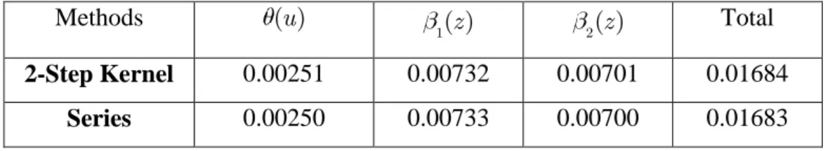
The simulation results are displayed in Table 1. Note that, the last column in Table 1 shows the sum of the three RMSE. From Table 1, we observe that the series and the two-step kernel methods give similar estimation results for the three functional coefficients. Consequently, both the series and two-step kernel methods can be a useful tool in estimating the FCPLR model. Next, we evaluate the 95% empirical coverage probabilities of the functional coefficients based on Theorem 2. Specifically, for a given value of u and z, the 95% confident intervals for ( )u

10 and _j( ),z j 1,2, are computed as ˆ( )u 2sˆ_u where sˆ_u Vˆ_u and ˆ_j 2sˆ_zjj where

ˆ ˆjj jj

z z

s V with Vˆ_zjj is the jth diagonal element of the matrix Vˆ_z. For simplicity, we evaluate these quantities at three different quantiles of u and z: 25%, 50% and 75%. In addition, since undersmoothing is required, we first assume L K for all cases, and use L (1.5 ,2.5 )L* L* as the number of approximating terms, where L* is the optimal value selected by using CV procedure. The results are displayed in Table 2. Our results indicated that the coverage probabilities of interval estimates based on the series estimators are very close to the true coverage probabilities and there are very little distortions.

4. Concluding Remark

In this paper, we propose an alternative and complementing approach for estimating the FCPLR model. Specially, we suggest a series method which is simpler to implement in practice than the kernel method. We established a synthesis on the consistency and asymptotic normality of the proposed estimator. Limited Monte Carlo simulations suggested the proposed estimator perform well in finite sample.

Note that, in practical application where we have dependent time series and this may not fit the general setting of this paper where the data are assumed to be independent. For dependent time series data, we conjecture that our approach can be still be applied to geometrically -mixing and strictly stationary data; and under a different set of regularity conditions (especially on the boundedness conditions), the convergence rate of the estimator still hold, although the asymptotic variance may have a different forms. Extension our approach to dependent time series data and perhaps dynamic panel data (see Lee (2013) and Tran (2014)) are interesting problems and deserves further research.

11 References

Ahmad, I., S. Leelahanon and Q. Li (2005). Efficient estimation of a semiparametric partially linear varying coefficient model. Ann. Statist. 33: 258-283.

Fan, J. and W. Zhang (2008). Statistical methods with varying coefficient models. Statistics and

Its Interface. 1: 179-195.

Hansen, B.E. (2012). Nonparametric sieve regression: least squares, averaging least squares, and cross-validation. Handbook of Applied Nonparametric and Semiparametric Econometrics

and Statistics. Chapter 8: 215-248.

Hansen, B.E. (2013). Econometrics. Mimeo, Department of Economics, University of Wisconsin, Madison WI.

Huang, J. Z. (2003). Local asymptotics for polynomial spline regression. Ann. Statist. 31: 1600-1635.

Lee, Y. (2013). Nonparametric estimation of dynamic panel models with fixed effect.

Econometric Theory. 30: 1315-1347.

Newey, W. K. (1997). Convergence rates and asymptotic normality for series estimators. J. of

Econometrics. 79: 147-168.

Tran, K.C. (2014). Nonparametric estimation of functional-coefficient partially linear dynamic panel data models with fixed effects. Economics Bulletin. 34(3): 1751-1761.

Wong, H., R. Zhang, W-C Ip and G. Li (2008). Functional-coefficient partially linear regression model. J. of Mult. Anal. 99: 278-305.

12

Appendix A:

Mathematical Proofs

First we present some useful lemmas which are the results that will be used in the proofs of Theorem1 and Theorem 2. Following the arguments of Newey (1997), we will assume without loss of generality, that A I_L and B I_K where I_R is an identity matrix of dimension R; A and B are defined in Assumptions 2 and 3. Thus, P uL( ) p u Q x zL( ), K( , ) q x zK( , ) and

'

[ ( ) ( ) ]L L L E p u p u IL,

'

[ K( , ) ( , ) ]K

K E q x z q x z IK. Also, we define an indicator

function 1_n which equals to 1 if (W W' ) is nonsingular and 0 otherwise, for W P or Q.

Lemma A.1 ( )i ˆ_L I_L O_p( ( )₀ L L n/ ) o_p(1);

( )ii ˆ_K I_K O_p( ( )₀ K K n/ ) o_p(1)

where ˆ_L P P n' / and ˆ_K QQ n' / .

PROOF: See Theorem 1 of Newey (1997).

Lemma A.2 ( )i 2 ( 20)

p

O L where (P P' ) 1P' , satisfies Assumption 4.

( )ii 2 ( d ₁ 2j)

g g Op j kj where

' 1 '

(QQ QG) , _g satisfies Assumption 5.

PROOF: The proof follows the same arguments as in the proof of Lemma A.2 in Ahmad et

al. (2005). Lemma A.3 ( )i 2 ' 1 ' 1 (_n P P n/ ) (P e n/ ) O L n_p( / ) ( )ii _{1 (} ' _{/ ) (}1 ' _{/ )}2 _{( / )} n QQ n Qe n O K np

13

PROOF: To prove ( )i , taking the conditional expectation of ( )i , we have

2 ' 1 ' [1 (_n / ) ( / ) | , , ] E P P n P e n u x z 1 {[(_nE e P n P P n' / )( ' / ) (1 P P n' / ) (1 P e n' / )] | , , }u x z O_p(1)1_ntr P P P( ( ' ) 1P E ee u x z' ( ' | , , ) / )n O_p(1)1 ( / )_nC L n

by Lemma A.1 and Assumption 1. Thus,

2

' 1 '

1 (_n P P n/ ) (P e n/ ) O L n_p( / ). The proof of ( )ii follows similarly.

Lemma A.4 ˆ _p 0 where ˆ n 1 _in₁[ ( ),p u q x zL _i K( , )][( ( ),_{i i} p u q x zL _i K( , )]_{i i} '

PROOF: First note that by Assumption 6 and by using argument as in Newey (1997),

without loss of generality we set  I where I is an identity matrix of dimension (L K ). Then it can be shown that as in Lemma 1, ˆ O_{p 0}(L K) (L K) /n o_p(1).

Proof of Theorem 1: The basic idea of the proof of this theorem is mainly from Newey (1997) and Ahmad et al. (2005).

( )i By (2) and (3), we can write

' 1 ' ' 1 ' ' 1 ' ' 1 ' ' 1 ' ' 1 ' ˆ ( ) ( ˆ) ˆ ( ) ( ( ) ( ) ) ˆ ( / ) ( / ) ( / ) ( ( ) / ) ( / ) ( ( ) / ) ˆ ( / ) ( ( ) / ) P P P Y Q P P P P Q e P G Q Q P P n P e n P P n P P n P P n P G Q n P P n P Q n Hence,

14 2 2 2 _{' 1 ' ' 1 '} 2 ' 1 ' 2 ' 1 ' ˆ 1 1 ( / ) ( / ) ( / ) ( ( ) / ) 1 ( / ) ( ( ) / ) ˆ 1 ( / ) ( ( ) / ) n n n n P P n P e n P P n P P n P P n P G Q n P P n P Q n

The first term 1 (_n P P n' / ) (1 P e n' / ) 2 O L n_p( / ) by Lemma A.3( )i . The second term 0

2 ₂

' 1 '

1 (_n P P n/ ) ( (P P ) / )n O L_p( ) by Lemma A.2( )i . Similarly, it is straightforward to show that the third term

2 ₂

' 1 '

1

1 ( / ) ( ( ) / ) ( d j)

n P P n P G Q n Op j kj

because the function G is approximated by Q and hence, the convergence rate will depend on

1

d j j

K k . The last term looks more complicated because it involves the convergence rate of ˆ

( ). However from (4), (ˆ )can be expressed explicitly as a function of (ˆ ) and by substituting this expression into the last term and solve for (ˆ ), it can be shown that

2

' 1 ' _ˆ

1 (_n P P n/ ) (PQ( ) / )n O K n_p( / ). Thus, by combining the above results, also by noting that 1_n 1 almost surely, we have

0 2 2 2 1 ˆ (( / ) ( / ) ( d j)) p j j O L n K n L k (A.1)

Next, by triangle inequality, we have

0 0 0 2 ' ' 2 2 _{' 2} 2 2 2 1 2 2 1 ˆ _ˆ [ ( ) ( )] ( ) [ ( ) ( ) ( ( ) ( ))] ( ) ˆ [ ( ) ( )] ( ) (( / ) ( / ) ( )) ( ) (( / ) ( / ) ( )) j j L L u u L u d p j j d p j j u u dF u p u p u u dF u p u u dF u O L n K n L k O L O L n K n L k

15 by (A.1), Lemma A.1 and Assumption 4( )i . Thus, we have proved Theorem 1( )i . The proof of Theorem 1( )ii follows the same arguments as in the proof above and hence omitted here. Proof of Theorem 2: The detailed proof of this theorem is a straightforward extension of the Theorems 2 and 3 of Newey (1997), so we discuss the heuristic idea of the proof here. First observe that ' 1 ' ' 1 ' ' 1 ' ˆ _ˆ 1 ( ( ) ( )) 1 ( ) 1 {( ) ( )} 1 {( ) ( )} 1 {( ) } n n n Q Q n Q Q n Q Q n u u nP nP P M P P M P nP P M P P M G Q nP P M P P M e (A.2) and ' 1 ' ' 1 ' ' 1 ' ˆ _ˆ 1 ( ( ) ( )) 1 ( ) 1 {( ) ( )} 1 {( ) ( )} 1 {( ) } n n n P P n P P n P P n z z nQ nQ Q M Q Q M G Q nQ Q M Q Q M P nQ Q M Q Q M e (A.3)

By Lemma A.4, we have ˆ _p 0 as n , thus, the first two terms in ( .2)A and ( .3)A can be shown to be asymptotically negligible by Assumptions A.4 and A.5. By combining the last term in ( .2)A and ( .3)A along with the result of partitioned regression, yields

' 1 ' ' 1 ' 1 ' ' 1 {( ) } 0 _ˆ 1 / 0 1 {( ) } 1 / n Q Q n n P P n nP P M P P M e P P e n Q nQ Q M Q Q M e Q e n

16 First note that ˆ 1 1 _p 0 as n . Second, following Newey (1997, proof of Theorem 3) and the fact that 1_n 1 almost surely, the limit distribution of the quantity

' '

/ / P e n

Q e n is approximately normal with mean zero and variance

2_{( , , )x u z}

. By using the

inverse matrix formula of the partitioned matrix, we have

1 _{1 1 1} 1 | | 1 1 1 1 1 1 | | 1 1 1 1 1 1 | | 1 1 1 | | pp pq pp q pp q pq qq qp qq qq qp pp q qq qq qp pp q pq qq pp pp pq qq p qp pp pp pq qq p qq p qp pp qq p

17 Table 1: RMSE of Functional Coefficients

Methods ( )u

1( )z 2( )z Total

2-Step Kernel 0.00251 0.00732 0.00701 0.01684 Series 0.00250 0.00733 0.00700 0.01683

Table 2: 95% Coverage Probabilities Quantile of u or z ( )u 1( )z 2( )z * 1.5 L L _{L 2.5L}* _{L 1.5L}* _{L 2.5L}* _{L 1.5L}* _{L 2.5L}* 0.25 0.952 0.951 0.951 0.950 0.953 0.952 0.50 0.957 0.950 0.954 0.955 0.953 0.952 0.75 0.952 0.953 0.951 0.953 0.953 0.956