Towards Informed Exploration for Deep Reinforcement Learning

(1)

UC Berkeley

UC Berkeley Electronic Theses and Dissertations

Permalink https://escholarship.org/uc/item/0pg0t84b Author Tang, Haoran Publication Date 2019 Peer reviewed|Thesis/dissertation

(2)

by

Haoran Tang

A dissertation submitted in partial satisfaction of the

requirements for the degree of

Doctor of Philosophy in Applied Mathematics in the Graduate Division of the

University of California, Berkeley

Committee in charge:

Professor James Sethian, Co-chair Professor Pieter Abbeel, Co-chair

Professor Trevor Darrell Associate Professor Lin Lin

(3)

(4)

Abstract

by Haoran Tang

Doctor of Philosophy in Applied Mathematics University of California, Berkeley

Professor James Sethian, Co-chair Professor Pieter Abbeel, Co-chair

In this thesis, we discuss various techniques for improving exploration for deep reinforcement learning. We begin with a brief review of reinforcement learning (RL) and the fundamental exploration v.s. exploitation trade-off. Then we review how deep RL has improved upon classical methods and summarize six categories of the latest exploration methods for deep RL, in the order of increasing usage of prior information. We then explore representative works in three categories and discuss their strengths and weaknesses. The first category, represented by Soft Q-learning, uses entropy regularization to encourage exploration. The second category, represented by count-based exploration via hashing, maps states to hash codes for counting and assigns higher exploration bonuses to less-encountered states. The third category utilizes hierarchy and is represented by a modular architecture for RL agents to play StarCraft II. Finally, we conclude that exploration informed by prior knowledge is a promising research direction and suggest topics of potentially high impact.

(5)

Acknowledgments

I am extremely fortunate to study in Applied Math as a PhD student at UC Berkeley. I am very grateful to Prof. James Sethian, who introduced me to the exciting field of applied math, offered generous help in my PhD program application, and guided me through my earlier years of study. I would also like to thank Prof. Pieter Abbeel especially, who has offered constant support and advice to help me transition into the field of deep reinforcement learning and to make this thesis possible. I am very thankful to Rocky Duan, Peter Chen, and Sergey Levine for their long-term guidance on my research. Thanks to my other collaborators for the work in this thesis, including Tuomas Haarnoja, Rein Houthooft, Davis Foote, Adam Stooke, Huazhe Xu, Dennis Lee, and Jeffrey O Zhang. Thanks to Lawrence Evans for serving on my quals committee, Trevor Darrell for serving on my dissertation committee, and Lin Lin for serving on both committees. Thanks to talented colleagues at UC Berkeley and DeepMind, including Carlos Florensa, Xinyang Geng, Tianhao Zhang, Yang Gao, Yi Wu, Keiran Paster, Yuhuai Wu, and Sasha Vezhnevets, for exchanging great research ideas. Thanks to my closest friends, Renyuan Xu, Difei Xiao, and Yingxin Chen for constant career and emotional guidance.

Finally, this thesis is dedicated to my parents Shuhuai Bi and Dengfeng Tang, for all the years of unconditional love and support.

(6)

Contents

Contents ii

1 Introduction 1

1.1 Reinforcement Learning . . . 1

1.2 The Exploration and Exploitation Trade-Off . . . 1

1.3 Deep Reinforcement Learning . . . 2

1.4 Techniques for Exploration in Deep Reinforcement Learning . . . 3

1.5 Contributions of This Thesis . . . 4

2 Reinforcement Learning with Deep Energy-Based Policies 6 2.1 Introduction . . . 6

2.2 Preliminaries . . . 8

2.3 Training Expressive Energy-Based Models via Soft Q-Learning . . . 10

2.4 Related Work . . . 14

2.5 Experiments . . . 15

2.6 Theoretical results . . . 19

2.7 Implementation Details . . . 23

2.8 Discussion . . . 25

3 #Exploration: A Study of Count-Based Exploration for Deep Reinforcement Leaning 26 3.1 Introduction . . . 26

3.2 Methodology . . . 27

3.4 Experiments . . . 31

3.5 A Case Study of Montezuma’s Revenge . . . 37

3.6 Discussion . . . 37

4 Modular Architecture for StarCraft II with Deep Reinforcement Learning 40 4.1 Introduction . . . 40

4.3 Modular Architecture . . . 42

(7)

4.5 Evaluation . . . 48 4.6 Discussion . . . 51

5 Conclusion 52

(8)

Chapter 1

Introduction

1.1

Reinforcement Learning

Reinforcement Learning (RL) is a trial-and-error framework for solving Markov Decision Processes (MDPs) [108]. An MDP consists of a state space S, an action space A, a transition function

p : S × A × S → [0,∞)s.t. R p(s,a,s0)ds0 = 1∀s,adescribing the probability of reaching a new state s0 after taking action a at state s, and a reward function r(s,a) received after the transition (some MDPs considerrstochastic). A (stochastic) policyπ :S × A → [0,∞)specifies a distribution over actionaat states. A typical objective for an MDP is to maximize the discounted sum of rewards max π Eπ,p " _∞ X t=0 γtr(st,at) # (1.1)

RL usually refers to model-free RL, which assumes no or little prior knowledge of S, A, p, or r. In particular, the only available tool is an environment simulator that returns sampled trajectories (sequences of states and actions) for a given policy. Intuitively, a policy identifies patterns through trials, increases the probabilities of more rewarding actions, and repeats the process until it converges. Q-learning [108] is a classic example for this trial-and-error approach. As we shall see in Section 1.2, the generality of RL comes at the cost of sample inefficiency and usually requires careful algorithmic design.

Here we further define several useful terms. A trajectory is τ = {(st,at)}Tt=0. The Q-value

for a policyπ isQπ_(s_,_{a) =}

Eπ,p[

P∞

t=0γ

t_r_(s

t,at)|s0 =s,a0 =a]. The value forπ is Vπ(s) =

Ea∼π(s,·)[Qπ(s,a)]. Q∗ andV∗correspond to the optimal policyπ∗.

1.2

The Exploration and Exploitation Trade-Off

During RL training, to guarantee convergence to the global optimum, each action at each state requires sufficient trials to accurately evaluate its outcome. But to accelerate convergence, the evaluation should be focused on (as currently perceived) more promising actions. The classic UCB1

(9)

algorithm summarizes such exploration v.s. exploitation trade-off in a multi-armed bandit (stateless MDP) setting. ak= arg max a ˆrk(a) +c s 2 logk Nk−1(a) ! (1.2)

where k is the number of iterations, rˆis the sample mean estimate of (stochastic) r, N is the number of timesahas been tried, andcis a tunable positive constant. Here the reward estimaterˆk

emphasizes exploitation, while the remaining term favors under-explored actions, hence encourages exploration. A similar version is used in the Monte-Carlo Tree Search algorithm for the famous AlphaGo agent [102].

In MDPs with longer horizons, the trade-off becomes even more crucial. Since the total reward estimation has higher variance, exploitation is more likely to lead to local optimum. Moreover, exploration becomes harder due to the increasing number of branching factors. Numerous theoretical attempts have been made to address the trade-off in finiteSandAsettings, many resembling (1.2) in certain ways. They will be discussed in more detail in Section 3.3, but here let us preview a representative algorithm and understand the complexity.

MIBE-EB [106] is a count-based method for exploration. At each timestep k, it counts the occurrenceN of each state-action pair, computes sample estimatesˆr,pˆof the reward and transition function, and solves an approximate Q-value that includes a bonus term for under-explored state-action pairs. Qk(s,a) = ˆrk(s,a) +γ X s0 ˆ pk(s,a,s0) max a0 Qk(s 0 ,a0) + _p β Nk(s,a) (1.3)

Thenak = arg maxaQk(sk,a)is executed at timestep k. This algorithm is "Provably

Approx-imately Correct", in the sense that an MDP-dependent coefficient β > 0 exists such that with probability(1−δ)(across all runs of the algorithm),Vπk_(s

k)≥V∗(sk)−εfor all but a polynomial

in(1/ε,1/δ,1/(1−γ),|S|,|A|)timesteps. In particular, convergence is almost guaranteed in the limit, but near-optimal solution is unlikely guaranteed without massive sampling. This example shows why solving RL thoroughly is a fundamentally difficult.

Beware that most theoretical works focus on finite (and small) MDPs. Problems with continuous

Sand/orApresent different opportunities and challenges. For example, imagery states are no longer treated distinct by minor differences in pixel values, but are compared by their visual semantics. On the other hand, the naive counting or sample mean estimates no longer work and different modeling techniques are required. For certain hard problems, one can even utilize prior knowledge to inform exploration. Section 1.4 will summarize such modern techniques.

1.3

Deep Reinforcement Learning

While traditional RL focuses on tabular or linear representations ofS and A, it is less effective against more complex problems, such as image observations. With the advance of deep learning [28], neural networks arise as powerful function approximators that can handle high-dimensional

(10)

inputs and outputs. Soon they became popular candidates for value functions and policies, and have been successfully applied to playing Atari games [68], mastering the game of Go [102], and learning locomotion controllers [96, 60].

The most popular deep RL methods are policy gradient [96, 66, 94, 34] and Q-learning [69, 60, 33]. Unlike classical algorithms, they are distinctively model-free, scalable, and data-intensive. In fact, the ability to utilize massive data is the major reason for the success of deep RL.

1.4

Techniques for Exploration in Deep Reinforcement

Learning

Techniques for exploration in deep RL are not fundamentally different from their classic coun-terparts. However, due to nonlinear function approximations, quantities such as(s,a)visitation frequency and variance of value estimates are not straightforward to obtain. Moreover, neural net-works are able to generalize to different inputs, the analysis of which has been absent in traditional RL, and still remains unsolved even in deep learning.

Nevertheless, variants of classic methods still have empirical utility. There exists a spectrum of techniques, from the least to the most informed (i.e. armed with prior knowledge), which we shall summarize here.

1. Entropy regularization. Initiated in [66] and later formalized in [33], this method prevents early convergence to a deterministic policy by introducing policy entropy to the objective. Chapter 2 will discuss it in more detail.

2. Novelty bonus. These techniques characterize novel or under-explored events, such as new

s,(s,a), or(s,a,s0), and assigns a bonus reward based on their novelty. This category of techniques has many names, such as count-based exploration [7], intrinsic motivation [41, 2], curiosity [84, 10], information gain [12], and others [26, 9]. Novelty bonus is by far the most popular research topic due to their effectiveness and generality.

3. Hierarchy. Hierarchical policies are thought to explore more efficiently, because the higher level can reason in longer horizons and in higher-level semantics. Successful examples include [55, 119, 22, 70].

4. Reward shaping. For certain challenging problems, such as MDPs with sparse rewards and long horizons, it can be easier to learn from a different but correlated reward. A famous example is presented in the OpenAI Dota project [78].

5. Bootstrapping from demonstrations. Sometimes the optimal solutions are so hard to search by RL that bootstrapping from demonstration is almost necessary. For example, self-play RL on StarCraft II was only able to learn naive rushing strategies. But by imitating expert actions and then learning from RL, the AlphaStar agent quickly surpassed human[120].

(11)

6. Meta-exploration. Meta-learning considers how to learn a new task quickly by leveraging knowledge from previously learned tasks. In particular, meta-exploration can acquire an exploration strategy from its learning experiences on other tasks. [17] and [32] have successful examples.

1.5

Contributions of This Thesis

In following chapters, we will see examples of detailed investigations into three types of exploration techniques: entropy regularization, novelty bonus, and hierarchy. The chosen order represents the author’s growing interest towards more informed exploration (more prior knowledge). Chapter 5 will summarize lessons learned from the investigations and argue why informed exploration is important for solving challenging problems efficiently in deep RL.

The first contribution, titled “Reinforcement Learning with Deep Energy-Based Policies”, studies how entropy regularization assists exploration. Drawing inspiration from stochastic opti-mal control, it proves that the optiopti-mal policy of the entropy-regularized objective has an energy formπ_soft∗ (s,a)∝a exp(Q∗soft(s,a)). Moreover,Q

∗

soft is the unique solution to the “soft Bellman

equation”, and therefore can be obtained from “soft Q-learning”, analogous to the conventional Q-learning. In addition,π_soft∗ uses a deep neural net to approximate the arbitrarily complex energy distribution, and is trained by Stein Variational Gradient Descent. Compared to the conven-tional Gaussian noise for greedy exploration, an energy-based policy assigns equal probabilities to equally rewarding actions, hence capturing various modes of good behavior. Experiments on continuous control tasks demonstrate its benefits on improved exploration and transfer learn-ing. Videos of related experiments are available athttps://sites.google.com/view/ softqlearning/home. The source code can be accessed at https://github.com/ haarnoja/softqlearning. A BAIR blog post summarizes key results along with new investi-gations: https://bair.berkeley.edu/blog/2017/10/06/soft-q-learning. This paper was published at 2017 International Conference on Machine Learning.

The second contribution, titled “#Exploration: A Study of Count-Based Exploration for Deep Reinforcement Leaning”, studies how to implement count-based exploration via simple hash functions. The paper begins by reviewing classic count-based exploration methods with “provably approximately correct” guarantees. It then proposes bonus rewards of the form √ β

n(φ(s)) to drive

the agent towards under-explored states. The key is choosing a good hash functionφ. It can be static and as simple as random projections. It can also be learned and represented by convolutional neural nets. Detailed experiments were performed on continuous control tasks from OpenAI Gym and challenging video games from Atari 2600. The simple hashing technique shows surprisingly competitive performance. A further investigation into Montezuma’s Revenge shows how designing hash functions that only incorporate task-related information can boost scores dramatically. Videos of related experiments are available at https://www.youtube.com/playlist?list= PLAd-UMX6FkBQdLNWtY8nH1-pzYJA_1T55. This work was published at 2017 Conference on Neural Information Processing Systems.

(12)

The third contribution, titled “Modular Architecture for StarCraft II with Deep Reinforcement Learning”, studies how to simplify complex exploration problems by modularization, pretraining, and hierarchy. The game-play agent consists of five modules, each responsible for a relatively independent subtask. A module is first pretrained with other handcrafted modules, and then combined with other pretrained modules for fine-tuning. A hierarchical structure lets each module choose macro actions (predefined action sequences) instead of raw actions, which greatly reduces the search space. The agent is trained to play StarCraft II by competing against itself. Without ever seeing the test opponents, it is able to beat the “Harder” difficulty built-in bot with a 92% success rate. A video of the learned agent’s self-play can be viewed at https://sites.google. com/view/modular-sc2-deeprl. This work was published at The 14th AAAI Conference on Artificial Intelligence and Interactive Digital Entertainment (2018).

(13)

Chapter 2

Reinforcement Learning with Deep

Energy-Based Policies

2.1

Introduction

Deep reinforcement learning (deep RL) has emerged as a promising direction for autonomous acquisition of complex behaviors [68, 102], due to its ability to process complex sensory input [43] and to acquire elaborate behavior skills using general-purpose neural network representations [59]. Deep reinforcement learning methods can be used to optimize deterministic [60] and stochastic [96, 66] policies. However, most deep RL methods operate on the conventional deterministic notion of optimality, where the optimal solution, at least under full observability, is always a deterministic policy [108]. Although stochastic policies are desirable for exploration, this exploration is typically attained heuristically, for example by injecting noise [101, 60, 68] or initializing a stochastic policy with high entropy [47, 96, 66].

In some cases, we might actually prefer to learn stochastic behaviors. In this chapter, we explore two potential reasons for this: exploration in the presence of multimodal objectives, and compositionality attained via pretraining. Other benefits include robustness in the face of uncertain dynamics [127], imitation learning [128], and improved convergence and computational properties [30]. Multi-modality also has application in real robot tasks, as demonstrated in [16]. However, in order to learn such policies, we must define an objective that promotes stochasticity.

In which cases is a stochastic policy actually the optimal solution? As discussed in prior work, a stochastic policy emerges as the optimal answer when we consider the connection between optimal control and probabilistic inference [112]. While there are multiple instantiations of this framework, they typically include the cost or reward function as an additional factor in a factor graph, and infer the optimal conditional distribution over actions conditioned on states. The solution can be shown to optimize an entropy-augmented reinforcement learning objective or to correspond to the solution to a maximum entropy learning problem [115]. Intuitively, framing control as inference produces policies that aim to capture not only the single deterministic behavior that has the lowest cost, but the entire range of low-cost behaviors, explicitly maximizing the entropy of the corresponding policy. Instead of learning the best way to perform the task, the resulting policies try to learnallof the ways of performing the task. It should now be apparent why such policies might be preferred: if

(14)

we can learn all of the ways that a given task might be performed, the resulting policy can serve as a good initialization for finetuning to a more specific behavior (e.g. first learning all the ways that a robot could move forward, and then using this as an initialization to learn separate running and bounding skills); a better exploration mechanism for seeking out the best mode in a multi-modal reward landscape; and a more robust behavior in the face of adversarial perturbations, where the ability to perform the same task in multiple different ways can provide the agent with more options to recover from perturbations.

Unfortunately, solving such maximum entropy stochastic policy learning problems in the general case is challenging. A number of methods have been proposed, including Z-learning [113], maximum entropy inverse RL [128], approximate inference using message passing [115],

Ψ-learning [88], and G-learning [24], as well as more recent proposals in deep RL such as PGQ [74], but these generally operate either on simple tabular representations, which are difficult to apply to continuous or high-dimensional domains, or employ a simple parametric representation of the policy distribution, such as a conditional Gaussian. Therefore, although the policy is optimized to perform the desired skill in many different ways, the resulting distribution is typically very limited in terms of its representational power, even if theparametersof that distribution are represented by an expressive function approximator, such as a neural network.

How can we extend the framework of maximum entropy policy search to arbitrary policy distributions? In this chapter, we borrow an idea from energy-based models, which in turn reveals an intriguing connection between Q-learning, actor-critic algorithms, and probabilistic inference. In our method, we formulate a stochastic policy as a (conditional) energy-based model (EBM), with the energy function corresponding to the “soft” Q-function obtained when optimizing the maximum entropy objective. In high-dimensional continuous spaces, sampling from this policy, just as with any general EBM, becomes intractable. We borrow from the recent literature on EBMs to devise an approximate sampling procedure based on training a separate sampling network, which is optimized to produce unbiased samples from the policy EBM. This sampling network can then be used both for updating the EBM and for action selection. In the parlance of reinforcement learning, the sampling network is the actor in an actor-critic algorithm.

The principal contribution of this work is a tractable, efficient algorithm for optimizing arbitrary multimodal stochastic policies represented by energy-based models, as well as a discussion that relates this method to other recent algorithms in RL and probabilistic inference. In our experimental evaluation, we explore two potential applications of our approach. First, we demonstrate improved exploration performance in tasks with multi-modal reward landscapes, where conventional deter-ministic or unimodal methods are at high risk of falling into suboptimal local optima. Second, we explore how our method can be used to provide a degree of compositionality in reinforcement learning by showing that stochastic energy-based policies can serve as a much better initialization for learning new skills than either random policies or policies pretrained with conventional maximum reward objectives.

(15)

2.2

Preliminaries

In this section, we will define the reinforcement learning problem that we are addressing and briefly summarize the maximum entropy policy search objective. We will also present a few useful identities that we will build on in our algorithm, which will be presented in Section 2.3.

Maximum Entropy Reinforcement Learning

We will address learning of maximum entropy policies with approximate inference for reinforcement learning in continuous action spaces. Our reinforcement learning problem can be defined as policy search in an infinite-horizon Markov decision process (MDP), which consists of the tuple

(S,A, ps, r), The state spaceS and action spaceA are assumed to be continuous, and the state

transition probabilityps : S × S × A → [0, ∞)represents the probability density of the next

statest+1 ∈ Sgiven the current statest∈ S and actionat∈ A. The environment emits a reward

r:S × A → [rmin, rmax]on each transition, which we will abbreviate asrt,r(st,at)to simplify

notation. We will also useρπ(st)andρπ(st,at)to denote the state and state-action marginals of the

trajectory distribution induced by a policyπ(at|st).

Our goal is to learn a policy π(at|st). We can define the standard reinforcement learning

objective in terms of the above quantities as

π∗_std= arg max

π

X

t

E(st,at)∼ρπ[r(st,at)]. (2.1)

Maximum entropy RL augments the reward with an entropy term, such that the optimal policy aims to maximize its entropy at each visited state:

(2.2)

π∗_MaxEnt= arg max

π

X

t

E(st,at)∼ρπ[r(st,at)+αH(π(· |st))],

whereαis an optional but convenient parameter that can be used to determine the relative importance of entropy and reward.1 _{Optimization problems of this type have been explored in a number of}

prior works [48, 113, 128], which are covered in more detail in Section 2.4. Note that this objective differs qualitatively from the behavior of Boltzmann exploration [92] and PGQ [74], which greedily maximize entropy at the current time step, but do not explicitly optimize for policies that aim to reachstateswhere they will have high entropy in the future. This distinction is crucial, since the maximum entropy objective can be shown to maximize the entropy of the entire trajectory distribution for the policyπ, while the greedy Boltzmann exploration approach does not [128, 58]. As we will discuss in Section 3.4, this maximum entropy formulation has a number of benefits, such as improved exploration in multimodal problems and better pretraining for later adaptation.

If we wish to extend either the conventional or the maximum entropy RL objective to infinite horizon problems, it is convenient to also introduce a discount factorγto ensure that the sum of expected rewards (and entropies) is finite. In the context of policy search algorithms, the use of a

1_{In principle,}₁_/α_{can be folded into the reward function, eliminating the need for an explicit multiplier, but in} practice, it is often convenient to keepαas a hyperparameter.

(16)

discount factor is actually a somewhat nuanced choice, and writing down the precise objective that is optimized when using the discount factor is non-trivial [111]. We defer the full derivation of the discounted objective to Section 2.6, since it is unwieldy to write out explicitly, but we will use the discountγ in the following derivations and in our final algorithm.

Soft Value Functions and Energy-Based Models

Optimizing the maximum entropy objective in (2.2) provides us with a framework for training stochastic policies, but we must still choose a representation for these policies. The choices in prior work include discrete multinomial distributions [74] and Gaussian distributions [88]. However, if we want to use a very general class of distributions that can represent complex, multimodal behaviors, we can instead opt for using general energy-based policies of the form

π(at|st)∝exp (−E(st,at)), (2.3)

whereE is an energy function that could be represented, for example, by a deep neural network. If we use a universal function approximator forE, we can represent any distributionπ(at|st). There

is a close connection between such energy-based models andsoftversions of value functions and Q-functions, where we setE(st,at) =−_α1Qsoft(st,at)and use the following theorem:

Theorem 1. Let the soft Q-function be defined by Q∗_soft(st,at) =rt+E(st+1,...)∼ρπ " _∞ X l=1 γl(rt+l+αH(π∗MaxEnt(· |st+l))) # ,

and soft value function by

V_soft∗ (st) =αlog Z A exp 1 αQ ∗ soft(st,a0) da0. (2.4)

Then the optimal policy for (2.2) is given by π∗_MaxEnt(at|st) = exp 1 α(Q ∗ soft(st,at)−Vsoft∗ (st)) . (2.5)

Proof. See Section 2.6 as well as [127].

Theorem 1 connects the maximum entropy objective in (2.2) and energy-based models, where

1

αQsoft(st,at)acts as the negative energy, and

1

αVsoft(st)serves as the log-partition function. As

with the standard Q-function and value function, we can relate the Q-function to the value function at a future state via a soft Bellman equation:

Theorem 2. The soft Q-function in (2.4) satisfies the soft Bellman equation Q∗_soft(st,at) =rt+γEst+1∼ps[V

∗

soft(st+1)], (2.6)

(17)

Proof. See Section 2.6, as well as [127].

The soft Bellman equation is a generalization of the conventional (hard) equation, where we can recover the more standard equation asα →0, which causes (2.4) to approach a hard maximum over the actions. In the next section, we will discuss how we can use these identities to derive a Q-learning style algorithm for learning maximum entropy policies, and how we can make this practical for arbitrary Q-function representations via an approximate inference procedure.

2.3

Training Expressive Energy-Based Models via Soft

Q-Learning

In this section, we will present our proposed reinforcement learning algorithm, which is based on the soft Q-function described in the previous section, but can be implemented via a tractable stochastic gradient descent procedure with approximate sampling. We will first describe the general case of soft Q-learning, and then present the inference procedure that makes it tractable to use with deep neural network representations in high-dimensional continuous state and action spaces. In the process, we will relate this Q-learning procedure to inference in energy-based models and actor-critic algorithms.

Soft Q-Iteration

We can obtain a solution to (2.6) by iteratively updating estimates ofV_soft∗ andQ∗_soft. This leads to a fixed-point iteration that resembles Q-iteration:

Theorem 3. Soft Q-iteration. LetQsoft(·, ·)andVsoft(·)be bounded and assume that

R Aexp(

1

αQsoft(·,a

0₎₎_d_a0_<∞_{and that}_Q∗

soft <∞exists. Then the fixed-point iteration

Qsoft(st,at)←rt+γEst+1∼ps[Vsoft(st+1)], ∀st,at (2.7) Vsoft(st)←αlog Z A exp 1 αQsoft(st,a 0 ) da0,∀st (2.8)

converges toQ∗_softandV_soft∗ , respectively. Proof. See Section 2.6 as well as [24].

We refer to the updates in (2.7) and (2.8) as the soft Bellman backup operator that acts on the soft value function, and denote it byT. The maximum entropy policy in (2.5) can then be recovered by iteratively applying this operator until convergence. However, there are several practicalities that need to be considered in order to make use of the algorithm. First, the soft Bellman backup cannot be performed exactly in continuous or large state and action spaces, and second, sampling from the energy-based model in (2.5) is intractable in general. We will address these challenges in the following sections.

(18)

Soft Q-Learning

This section discusses how the Bellman backup in Theorem 3 can be implemented in a practical algorithm that uses a finite set of samples from the environment, resulting in a method similar to Q-learning. Since the soft Bellman backup is a contraction (see Section 2.6), the optimal value function is the fixed point of the Bellman backup, and we can find it by optimizing for a Q-function for which the soft Bellman error |TQ−Q| is minimized at all states and actions. While this procedure is still intractable due to the integral in (2.8) and the infinite set of all states and actions, we can express it as a stochastic optimization, which leads to a stochastic gradient descent update procedure. We will model the soft Q-function with a function approximator with parametersθand denote it asQθ

soft(st,at).

To convert Theorem 3 into a stochastic optimization problem, we first express the soft value function in terms of an expectation via importance sampling:

V_softθ (st) = αlogEqa0 " exp _α1Qθ soft(st,a0) qa0(a0) # , (2.9)

whereqa0 can be an arbitrary distribution over the action space. Second, by noting the identity g1(x) = g2(x) ∀x ∈ X ⇔ Ex∼q[(g1(x)−g2(x))2] = 0, whereq can be any strictly positive

density function on_X, we can express the soft Q-iteration in an equivalent form as minimizing

JQ(θ) = Est∼qs_t,at∼qa_t 1 2 ˆ Qθ_soft¯ (st,at)−Qθsoft(st,at) 2 , (2.10)

whereqst, qat are positive overS andArespectively,Qˆ

¯ θ soft(st,at) = rt+γEst+1∼ps[V ¯ θ soft(st+1)]is a

targetQ-value, withVθ¯

soft(st+1)given by (2.9) andθbeing replaced by the target parameters,θ¯.

This stochastic optimization problem can be solved approximately using stochastic gradient de-scent using sampled states and actions. While the sampling distributionsqstandqat can be arbitrary,

we typically use real samples from rollouts of the current policyπ(at|st)∝exp _α1Qθsoft(st,at)

. Forqa0 we have more options. A convenient choice is a uniform distribution. However, this choice

can scale poorly to high dimensions. A better choice is to use the current policy, which produces an unbiased estimate of the soft value as can be confirmed by substitution. This overall procedure yields an iterative approach that optimizes over the Q-values, which we summarize in Section 2.3. However, in continuous spaces, we still need a tractable way to sample from the policy

π(at|st) ∝ exp _α1Qθsoft(st,at)

, both to take on-policy actions and, if so desired, to generate action samples for estimating the soft value function. Since the form of the policy is so general, sampling from it is intractable. We will therefore use an approximate sampling procedure, as discussed in the following section.

Approximate Sampling and Stein Variational Gradient Descent (SVGD)

In this section we describe how we can approximately sample from the soft Q-function. Existing approaches that sample from energy-based distributions generally fall into two categories: methods that use Markov chain Monte Carlo (MCMC) based sampling [92], and methods that learn a stochastic sampling network trained to output approximate samples from the target distribution

(19)

[126, 50]. Since sampling via MCMC is not tractable when the inference must be performed online (e.g. when executing a policy), we will use a sampling network based on Stein variational gradient descent (SVGD) [61] and amortized SVGD [122]. Amortized SVGD has several intriguing properties: First, it provides us with a stochastic sampling network that we can query for extremely fast sample generation. Second, it can be shown to converge to an accurate estimate of the posterior distribution of an EBM. Third, the resulting algorithm, as we will show later, strongly resembles actor-critic algorithm, which provides for a simple and computationally efficient implementation and sheds light on the connection between our algorithm and prior actor-critic methods.

Formally, we want to learn a state-conditioned stochastic neural network at = fφ(ξ;st),

parametrized byφ, that maps noise samplesξ drawn from a normal Gaussian, or other arbitrary distribution, into unbiased action samples from the target EBM corresponding toQθ

soft. We denote

the induced distribution of the actions asπφ_(a

t|st), and we want to find parametersφ so that the

induced distribution approximates the energy-based distribution in terms of the KL divergence

Jπ(φ;st) = DKL πφ(· |st) exp 1 α Q θ soft(st, ·)−Vsoftθ .

Suppose we “perturb” a set of independent samplesa(_ti) = fφ(ξ(i);st) in appropriate directions

∆fφ₍_ξ(i)_;_s

t), the induced KL divergence can be reduced. Stein variational gradient descent [61]

provides the most greedy directions as a functional

∆fφ(·;st) = Eat∼πφ h κ(at, fφ(·;st))∇a0Qθ soft(st,a0) a0₌_a t +α∇a 0κ(a0, fφ(·;s_t)) a0₌_a t i ,

whereκis a kernel function (typically Gaussian, see details in Section 2.7). To be precise,∆fφis the optimal direction in the reproducing kernel Hilbert space ofκ, and is thus not strictly speaking the gradient of (2.11), but it turns out that we can set ∂Jπ

∂at ∝∆f

φ_{as explained in [122]. With this}

assumption, we can use the chain rule and backpropagate the Stein variational gradient into the policy network according to

∂Jπ(φ;st) ∂φ ∝Eξ ∆fφ(ξ;st) ∂fφ(ξ;st) ∂φ , (2.11)

and use any gradient-based optimization method to learn the optimal sampling network parameters. The sampling networkfφcan be viewed as an actor in an actor-critic algorithm. We will discuss this connection in Section 2.4, but first we will summarize our complete maximum entropy policy learning algorithm.

Algorithm Summary

To summarize, we propose the soft Q-learning algorithm for learning maximum entropy policies in continuous domains. The algorithm proceeds by alternating between collecting new experience from the environment, and updating the soft Q-function and sampling network parameters. The experience is stored in a replay memory buffer Das standard in deep Q-learning [69], and the parameters are updated using random minibatches from this memory. The soft Q-function updates

(20)

use a delayed version of the target values [68]. For optimization, we use the ADAM [52] optimizer and empirical estimates of the gradients, which we denote by∇ˆ. The exact formulae used to compute the gradient estimates is deferred to Section 2.7, which also discusses other implementation details, but we summarize an overview of soft Q-learning in algorithm 1.

Algorithm 1:Soft Q-learning

θ, φ∼some initialization distributions. Assign target parameters: θ¯←θ,φ¯←φ.

D ←empty replay memory.

foreach epochdo foreachtdo

Collect experience

Sample an action forstusingfφ:

at←fφ(ξ;st)whereξ ∼ N(0,I).

Sample next state from the environment:

st+1 ∼ps(st+1|st,at).

Save the new experience in the replay memory:

D ← D ∪ {(st,at, r(st,at),st+1)}.

Sample a minibatch from the replay memory {(s(_ti),a(_ti), r_t(i),s(_t₊₁i) )}N

i=0 ∼ D.

Update the soft Q-function parameters

Sample{a(i,j)_}M

j=0∼qa0 for eachs(i)

t+1.

Compute empirical soft valuesVˆ_softθ¯ (s(_ti₊₁) )in (2.9). Compute empirical gradient∇ˆθJQof (2.10).

Updateθaccording to∇ˆθJQusing ADAM.

Update policy

Sample{ξ(i,j)_}M

j=0 ∼ N(0,I)for eachs (i)

t .

Compute actionsa(_ti,j) =fφ(ξ(i,j),s(_ti)).

Compute∆fφ_{using empirical estimate of (2.11).}

Compute empiricial estimate of (2.11): ∇ˆφJπ.

Updateφaccording to∇ˆφJπ using ADAM.

end for

ifepochmodupdate_interval= 0then

Update target parameters: θ¯←θ,φ¯←φ.

end if end for

(21)

2.4

Related Work

Maximum entropy policies emerge as the solution when we cast optimal control as probabilistic inference. In the case of linear-quadratic systems, the mean of the maximum entropy policy is exactly the optimal deterministic policy [112], which has been exploited to construct practical path planning methods based on iterative linearization and probabilistic inference techniques [115]. In discrete state spaces, the maximum entropy policy can be obtained exactly. This has been explored in the context of linearly solvable MDPs [113] and, in the case of inverse reinforcement learning, MaxEnt IRL [128]. In continuous systems and continuous time, path integral control studies maximum entropy policies and maximum entropy planning [48]. In contrast to these prior methods, our work is focused on extending the maximum entropy policy search framework to high-dimensional continuous spaces and highly multimodal objectives, via expressive general-purpose energy functions represented by deep neural networks. A number of related methods have also used maximum entropy policy optimization as an intermediate step for optimizing policies under a standard expected reward objective [87, 73, 88, 24]. Among these, the work of [88] resembles ours in that it also makes use of a temporal difference style update to a soft Q-function. However, unlike this prior work, we focus on general-purpose energy functions with approximate sampling, rather than analytically normalizable distributions. A recent work [liu2017stein] also considers an entropy regularized objective, though the entropy is on policy parameters, not on sampled actions. Thus the resulting policy may not represent an arbitrarily complex multi-modal distribution with a single parameter. The form of our sampler resembles the stochastic networks proposed in recent work on hierarchical learning [22]. However this prior work uses a task-specific reward bonus system to encourage stochastic behavior, while our approach is derived from optimizing a general maximum entropy objective.

A closely related concept to maximum entropy policies is Boltzmann exploration, which uses the exponential of the standard Q-function as the probability of an action [46]. A number of prior works have also explored representing policies as energy-based models, with the Q-value obtained from an energy model such as a restricted Boltzmann machine (RBM) [92, 19, 82, 39]. Although these methods are closely related, they have not, to our knowledge, been extended to the case of deep network models, have not made extensive use of approximate inference techniques, and have not been demonstrated on the complex continuous tasks. More recently, [74] drew a connection between Boltzmann exploration and entropy-regularized policy gradient, though in a theoretical framework that differs from maximum entropy policy search: unlike the full maximum entropy framework, the approach of [74] only optimizes for maximizing entropy at the current time step, rather than planning for visiting future states where entropy will be further maximized. This prior method also does not demonstrate learning complex multi-modal policies in continuous action spaces.

Although we motivate our method as Q-learning, its structure resembles an actor-critic algo-rithm. It is particularly instructive to observe the connection between our approach and the deep deterministic policy gradient method (DDPG) [60], which updates a Q-function critic according to (hard) Bellman updates, and then backpropagates the Q-value gradient into the actor, similarly to NFQCA [35]. Our actor update differs only in the addition of theκterm. Indeed, without this

(22)

term, our actor would estimate a maximum a posteriori (MAP) action, rather than capturing the entire EBM distribution. This suggests an intriguing connection between our method and DDPG: if we simply modify the DDPG critic updates to estimate soft Q-values, we recover the MAP variant of our method. Furthermore, this connection allows us to cast DDPG as simply an approximate Q-learning method, where the actor serves the role of an approximate maximizer. This helps explain the good performance of DDPG on off-policy data.

2.5

Experiments

Our experiments aim to answer the following questions: (1) Does our soft Q-learning method accurately capture a multi-modal policy distribution? (2) Can soft Q-learning with energy-based policies aid exploration for complex tasks that require tracking multiple modes? (3) Can a maximum entropy policy serve as a good initialization for finetuning on different tasks, when compared to pretraining with a standard deterministic objective? We compare our algorithm to DDPG [60], which has been shown to achieve better sample efficiency on the continuous control problems that we consider than other recent techniques such as REINFORCE [125], TRPO [96], and A3C [66]. This comparison is particularly interesting since, as discussed in Section 2.4, DDPG closely corresponds to a deterministic maximum a posteriori variant of our method. The detailed experimental setup can be found in Section 2.7. Videos of all experiments2 _{and example source code}3_{are available online.}

Didactic Example: Multi-Goal Environment

In order to verify that amortized SVGD can correctly draw samples from energy-based policies of the formexp Qθ

soft(s, a)

, and that our complete algorithm can successful learn to represent multi-modal behavior, we designed a simple “multi-goal” environment, in which the agent is a 2D point mass trying to reach one of four symmetrically placed goals. The reward is defined as a mixture of Gaussians, with means placed at the goal positions. An optimal strategy is to go to an arbitrary goal, and the optimal maximum entropy policy should be able to choose each of the four goals at random. The final policy obtained with our method is illustrated in Figure 2.1. The Q-values indeed have complex shapes, being unimodal ats = (−2,0), convex ats= (0,0), and bimodal ats= (2.5,2.5). The stochastic policy samples actions closely following the energy landscape, hence learning diverse trajectories that lead to all four goals. In comparison, a policy trained with DDPG randomly commits to a single goal.

Learning Multi-Modal Policies for Exploration

Though not all environments have a clear multi-modal reward landscape as in the “multi-goal” example, multi-modality is prevalent in a variety of tasks. For example, a chess player might try various strategies before settling on one that seems most effective, and an agent navigating a maze may need to try various paths before finding the exit. During the learning process, it is often best to keep trying multiple available options until the agent is confident that one of them is the best

2_{https://sites.google.com/view/softqlearning/home} 3_{https://github.com/haarnoja/softqlearning}

(23)

Figure 2.1: Illustration of the 2D multi-goal environment. Left: trajectories from a policy learned with our method (solid blue lines). The xand y axes correspond to 2D positions (states). The agent is initialized at the origin. The goals are depicted as red dots, and the level curves show the reward. Right: Q-values at three selected states, depicted by level curves (red: high values, blue: low values). Thex and yaxes correspond to 2D velocity (actions) bounded between -1 and 1. Actions sampled from the policy are shown as blue stars. Note that, in regions (e.g. (2.5,2.5)) between the goals, the method chooses multimodal actions.

(a) Swimming snake (b) Quadrupedal robot

Figure 2.2: Simulated robots used in our experiments.

(similar to a bandit problem [56]). However, deep RL algorithms for continuous control typically use unimodal action distributions, which are not well suited to capture such multi-modality. As a consequence, such algorithms may prematurely commit to one mode and converge to suboptimal behavior.

To evaluate how maximum entropy policies might aid exploration, we constructed simulated continuous control environments where tracking multiple modes is important for success. The first experiment uses a simulated swimming snake (see Figure 2.2), which receives a reward equal to its speed along thex-axis, either forward or backward. However, once the swimmer swims far enough

(24)

forward, it crosses a “finish line” and receives a larger reward. Therefore, the best learning strategy is to explore in both directions until the bonus reward is discovered, and then commit to swimming forward. As illustrated in Figure 2.3 in Figure 2.3, our method is able to recover this strategy, keeping track of both modes until the finish line is discovered. All stochastic policies eventually commit to swimming forward. The deterministic DDPG method shown in the comparison commits to a mode prematurely, with only 80% of the policies converging on a forward motion, and 20% choosing the suboptimal backward mode.

(a) DDPG (b) Soft Q-learning

Figure 2.3: Forward swimming distance achieved by each policy. Each row is a policy with a unique random seed. x: training iteration, y: distance (positive: forward, negative: backward). Red line: the “finish line.” The blue shaded region is bounded by the maximum and minimum distance (which are equal for DDPG). The plot shows that our method is able to explore equally well in both directions before it commits to the better one.

The second experiment studies a more complex task with a continuous range of equally good options prior to discovery of a sparse reward goal. In this task, a quadrupedal 3D robot (adapted from [95]) needs to find a path through a maze to a target position (see Figure 2.2). The reward function is a Gaussian centered at the target. The agent may choose either the upper or lower passage, which appear identical at first, but the upper passage is blocked by a barrier. Similar to the swimmer experiment, the optimal strategy requires exploring both directions and choosing the better one. Figure 2.4(b) compares the performance of DDPG and our method. The curves show the minimum distance to the target achieved so far and the threshold equals the minimum possible distance if the robot chooses the upper passage. Therefore, successful exploration means reaching below the threshold. All policies trained with our method manage to succeed, while only 60%

(25)

(a) Swimmer (higher is better) (b) Quadruped (lower is better)

Figure 2.4: Comparison of soft Q-learning and DDPG on the swimmer snake task and the quadrupedal robot maze task. (a) Shows the maximum traveled forward distance since the beginning of training for several runs of each algorithm; there is a large reward after crossing the finish line. (b) Shows our method was able to reach a low distance to the goal faster and more consistently. The different lines show the minimum distance to the goal since the beginning of training. For both domains, all runs of our method cross the threshold line, acquiring the more optimal strategy, while some runs of DDPG do not.

Accelerating Training on Complex Tasks with Pretrained Maximum

Entropy Policies

A standard way to accelerate deep neural network training is task-specific initialization [28], where a network trained for one task is used as initialization for another task. The first task might be something highly general, such as classifying a large image dataset, while the second task might be more specific, such as fine-grained classification with a small dataset. Pretraining has also been explored in the context of RL [98]. However, in RL, optimal policies are often near-deterministic, which makes them poor initializers for new tasks. In this section, we explore how our energy-based policies can be trained with fairly broad objectives to produce an initializer for more quickly learning more specific tasks.

We demonstrate this on a variant of the quadrupedal robot task. The pretraining phase involves learning to locomote in an arbitrary direction, with a reward that simply equals the speed of the center of mass. The resulting policy moves the agent quickly to an randomly chosen direction. An overhead plot of the center of mass traces is shown above to illustrate this. This pretraining is similar in some ways to recent work on modulated controllers [40] and hierarchical models [22]. However, in contrast to these prior works, we do not require any task-specific high-level goal generator or reward.

Figure 2.6 also shows a variety of test environments that we used to finetune the running policy for a specific task. In the hallway environments, the agent receives the same reward, but the walls block sideways motion, so the optimal solution requires learning to run in a particular direction.

(26)

Figure 2.5: Center of mass plot after quadruped pretraining.

Figure 2.6: Quadrupedal robot (a) was trained to walk in random directions in an empty pretraining environment (details in Figure 2.7), and then finetuned on a variety of tasks, including a wide (b), narrow (c), and U-shaped hallway (d).

Narrow hallways require choosing a more specific direction, but also allow the agent to use the walls to funnel itself. The U-shaped maze requires the agent to learn a curved trajectory in order to arrive at the target, with the reward given by a Gaussian bump at the target location.

As illustrated in Figure 2.7, the pretrained policy explores the space extensively and in all directions. This gives a good initialization for the policy, allowing it to learn the behaviors in the test environments more quickly than training a policy with DDPG from a random initialization, as shown in Figure 2.8. We also evaluated an alternative pretraining method based on deterministic policies learned with DDPG. However, deterministic pretraining chooses an arbitrary but consistent direction in the training environment, providing a poor initialization for finetuning to a specific task, as shown in the results plots.

2.6

Theoretical results

Here we present proofs for the theorems that allow us to show that soft Q-learning leads to policy improvement with respect to the maximum entropy objective. First, we define a slightly more nuanced version of the maximum entropy objective that allows us to incorporate a discount factor. This definition is complicated by the fact that, when using a discount factor for policy gradient methods, we typically do not discount the state distribution, only the rewards. In that sense,

(27)

10 5 0 5 10 10 5 0 5 10 10 5 0 5 10 10 5 0 5 10 10 5 0 5 10 10 5 0 5 10 10 5 0 5 10 10 5 0 5 10 10 5 0 5 10 10 5 0 5 10 10 5 0 5 10 10 5 0 5 10 10 5 0 5 10 10 5 0 5 10 10 5 0 5 10 10 5 0 5 10 10 5 0 5 10 10 5 0 5 10 10 5 0 5 10 10 5 0 5 10 10 5 0 5 10 10 5 0 5 10 10 5 0 5 10 10 5 0 5 10 10 5 0 5 10 10 5 0 5 10 10 5 0 5 10 10 5 0 5 10 10 5 0 5 10 10 5 0 5 10 10 5 0 5 10 10 5 0 5 10 10 5 0 5 10 10 5 0 5 10 10 5 0 5 10 10 5 0 5 10 10 5 0 5 10 10 5 0 5 10 10 5 0 5 10 10 5 0 5 10

Figure 2.7: The plot shows trajectories of the quadrupedal robot during maximum entropy pre-training. The robot has diverse behavior and explores multiple directions. The four columns correspond to entropy coefficientsα = 10,1,0.1,0.01respectively. Different rows correspond to policies trained with different random seeds. The x and y axes show the x and y coordinates of the center-of-mass. Asαdecreases, the training process focuses more on high rewards, therefore exploring the training ground more extensively. However, lowαalso tends to produce less diverse behavior. Therefore the trajectories are more concentrated in the fourth column.

(28)

Figure 2.8: Performance in the downstream task with fine-tuning (MaxEnt) or training from scratch (DDPG). Thex-axis shows the training iterations. The y-axis shows the average discounted return. Solid lines are average values over 10 random seeds. Shaded regions correspond to one standard deviation.

optimize average reward, with the discount serving to reduce variance, as discussed by [111]. However, for the purposes of the derivation, we can define the objective thatisoptimized under a discount factor as

π∗_MaxEnt= arg max

π X t E(st,at)∼ρπ " _∞ X l=t γl−t_E(sl,al)[r(st,at) +αH(π(· |st))|st,at] # .

This objective corresponds to maximizing the discounted expected reward and entropy for future states originating from every state-action tuple (st,at)weighted by its probability ρπ under the

current policy. Note that this objective still takes into account the entropy of the policy at future states, in contrast to greedy objectives such as Boltzmann exploration or the approach proposed by [74].

We can now derive policy improvement results for soft Q-learning. We start with the definition of the soft Q-value Qπ

soft for any policyπ as the expectation underπ of the discounted sum of

rewards and entropy :

Qπ_soft(s,a)_,r0+Eτ∼π,s0=s,a0=a " _∞ X t=1 γt(rt+H(π(· |st))) # . (2.12)

Here,τ = (s0,a0,s1,a1, . . .)denotes the trajectory originating at(s,a). Notice that for convenience,

we set the entropy parameterαto 1. The theory can be easily adapted by dividing rewards byα. The discounted maximum entropy policy objective can now be defined as

J(π)_,X

t

E(st,at)∼ρπ[Q

π

(29)

The Maximum Entropy Policy

If the objective function is the expected discounted sum of rewards, the policy improvement theorem [108] describes how policies can be improved monotonically. There is a similar theorem we can derive for the maximum entropy objective:

Theorem 4. (Policy improvement theorem) Given a policyπ, define a new policyπ˜as

˜

π(· |s)∝exp Qπsoft(s, ·)

, ∀s. (2.14)

Assume that throughout our computation,Qis bounded andR exp(Q(s,a))dais bounded for any

s(for bothπandπ). Then˜ Q˜π

soft(s,a)≥Qπsoft(s,a)∀s,a.

The proof relies on the following observation: if one greedily maximize the sum of entropy and value with one-step look-ahead, then one obtainsπ˜fromπ:

H(π(· |s)) +_Ea∼π[Qπsoft(s,a)]≤ H(π˜(· |s)) +Ea∼˜π[Qπsoft(s,a)]. (2.15)

The proof is straight-forward by noticing that

H(π(· |s)) +_Ea∼π[Qπsoft(s,a)] = −DKL(π(· |s)kπ˜(· |s)) + log

Z

exp (Qπ_soft(s,a)) da (2.16) Then we can show that

With Theorem 4, we start from an arbitrary policyπ0and define thepolicy iterationas

πi+1(· |s)∝exp (Qsoftπi (s, ·)). (2.19)

Then Qπi

soft(s,a) improves monotonically. Under certain regularity conditions, πi converges to

π∞. Obviously, we have π∞(a|s) ∝a exp (Qπ∞(s,a)). Since any non-optimal policy can be

improved this way, the optimal policy must satisfy this energy-based form. Therefore we have proven Theorem 1.

(30)

Soft Bellman Equation and Soft Value Iteration

Recall the definition of the soft value function:

V_softπ (s)_,log

Z

exp (Qπ_soft(s,a)) da. (2.20) Supposeπ(a|s) = exp (Qπ_soft(s,a)−V_softπ (s)). Then we can show that

Qπ_soft(s,a) =r(s,a) +γ_Es0_∼_p s H(π(· |s0)) +_Ea0_∼_π₍_{· |}_s0₎[Qπ soft(s 0 ,a0)] =r(s,a) +γ_Es0_∼_p s[V π soft(s 0 )]. (2.21)

This completes the proof of Theorem 2.

Finally, we show that the soft value iteration operatorT, defined as

TQ(s,a)_,r(s,a) +γ_Es0_∼_p s log Z expQ(s0,a0)da0 , (2.22)

is a contraction. Then Theorem 3 follows immediately.

The following proof has also been presented by [24]. Define a norm on Q-values askQ1−Q2k, maxs,a|Q1(s,a)−Q2(s,a)|. Supposeε=kQ1−Q2k. Then

log Z exp(Q1(s0,a0))da0 ≤log Z exp(Q2(s0,a0) +ε)da0 = log exp(ε) Z expQ2(s0,a0)da0 =ε+ log Z expQ2(a0,a0)da0. (2.23)

Similarly,logR expQ1(s0,a0)da0 ≥ −ε+ log

R

expQ2(s0,a0)da0. ThereforekTQ1− TQ2k ≤

γε =γkQ1−Q2k. SoT is a contraction. As a consequence, only one Q-value satisfies the soft

Bellman equation, and thus the optimal policy presented in Theorem 1 is unique.

2.7

Implementation Details

Hyperparameters

All tasks have a horizon ofT = 500, except the multi-goal task, which usesT = 20. We add an additional termination condition to the quadrupedal 3D robot to discourage it from flipping over.

Throughout all experiments, we use the following parameters for both DDPG and soft Q-learning. The Q-values are updated using ADAM with learning rate0.001. The DDPG policy and soft Q-learning sampling network use ADAM with a learning rate of0.0001. The algorithm uses a replay pool of size one million. Training does not start until the replay pool has at least 10,000 samples. Every mini-batch has size64. Each training iteration consists of10000time steps, and both

(31)

the Q-values and policy / sampling network are trained at every time step. All experiments are run for500epochs, except that the multi-goal task uses100epochs and the fine-tuning tasks are trained for200epochs. Both the Q-value and policy / sampling network are neural networks comprised of two hidden layers, with200hidden units at each layer and ReLU nonlinearity. Both DDPG and soft Q-learning use additional OU Noise [116, 60] to improve exploration. The parameters are

θ = 0.15andσ = 0.3. In addition, we found that updating the target parameters too frequently can destabilize training. Therefore we freeze target parameters for every1000time steps (except for the swimming snake experiment, which freezes for5000epochs), and then copy the current network parameters to the target networks directly (τ = 1).

Soft Q-learning uses K = M = 32action samples (see Section 2.7) to compute the policy update, except that the multi-goal experiment usesK =M = 100. The number of additional action samples to compute the soft value isKV = 50. The kernelκ is a radial basis function, written

as κ(a,a0) = exp(−1

hka−a

0_k2

2), whereh = 2 log(dM+1), withd equal to the median of pairwise

distance of sampled actionsa(_ti). Note that the step sizehchanges dynamically depending on the states, as suggested in [61].

The entropy coefficientαis10for multi-goal environment, and0.1for the swimming snake, maze, hallway (pretraining) and U-shaped maze (pretraining) experiments.

All fine-tuning tasks anneal the entropy coefficientαquickly in order to improve performance, since the goal during fine-tuning is to recover a near-deterministic policy on the fine-tuning task. In particular,αis annealed log-linearly to0.001within20epochs of fine-tuning. Moreover, the samplesξare fixed to a set{ξi}

Kξ

i=1andKξis reduced linearly to1within20epochs.

Computing the Policy Update

Here we explain in full detail how the policy update direction∇ˆφJπ in algorithm 1 is computed.

We reuse the indicesi, j in this section with a different meaning than in the body for the sake of providing a cleaner presentation.

Expectations appear in amortized SVGD in two places. First, SVGD approximates the optimal descent directionφ(·)in Equation (2.11) with an empirical average over the samplesa_t(i) =fφ(ξ(i)). Similarly, SVGD approximates the expectation in Equation (2.11) with samples˜a(_tj) =fφ( ˜ξ(j)), which can be the same or different froma(_ti). Substituting (2.11) into (2.11) and taking the gradient gives the empirical estimate

ˆ ∇φJπ(φ;st)=_KM1 PKj=1 PM i=1 κ(a(_ti),˜a_t(j))∇_a0Qsoft(st,a0) a0=a(_ti)+∇a0κ(a 0_,_a_˜(j) t ) a0=a(_ti) ∇φfφ( ˜ξ(j);st).

Finally, the update direction∇ˆφJπ is the average of∇ˆφJπ(φ;st), wherestis drawn from a

(32)

Computing the Density of Sampled Actions

Equation (2.9) states that the soft value can be computed by sampling from a distributionqa0and that qa0(·) ∝exp 1 αQ φ soft(s, ·)

is optimal. A direct solution is to obtain actions from the sampling network: a0 = fφ(ξ0;s). If the samples ξ0 and actions a0 have the same dimension, and if the jacobian matrix ∂_∂ξa00 is non-singular, then the probability density is

qa0(a0) =p_ξ(ξ0) 1 det ∂a0 ∂ξ0 . (2.24)

In practice, the Jacobian is usually singular at the beginning of training, when the samplerfφis not fully trained. A simple solution is to begin with uniform action sampling and then switch to

fφ_{later, which is reasonable, since an untrained sampler is unlikely to produce better samples for}

estimating the partition function anyway.

2.8

Discussion

In summary, Soft Q-Learning improves exploration by explicitly sampling actions fromexp(Qsoft−

Vsoft), thus trying similarly rewarding actions with similar probabilities and eventually avoiding

local minimums. However, in practice, sampling variation can still incorrectly favor less rewarding actions, which will cause early convergence through the snowball effect - more experiences are gathered using the worse actions, which in turn biases the Q-value estimate towards favoring them. Therefore the exploration vs exploitation conflict forces a trade-off between accurate value estimation and fast convergence.

To formalize the energy-based policy form, an entropy-regularized objective is proposed in place of total rewards. Despite its task-agnostic definition, it should be considered a modeling tool rather than an objective truth. Besides shaping the reward, one can easily change the optimal policy by remapping the action space or choosing a different temperatureα. Therefore, it is up to the user to decide the form and degree of exploration.

Entropy regularization has limited power since it only involves properties of the reward function. In later chapters, we will study how to inform exploration by exploiting the state-space structure Chapter 3 and the decision hierarchy Chapter 4.

(33)

Chapter 3

#Exploration: A Study of Count-Based

Exploration for Deep Reinforcement

Leaning

3.1

Introduction

Reinforcement learning (RL) studies an agent acting in an initially unknown environment, learning through trial and error to maximize rewards. It is impossible for the agent to act near-optimally until it has sufficiently explored the environment and identified all of the opportunities for high reward, in all scenarios. A core challenge in RL is how to balance exploration—actively seeking out novel states and actions that might yield high rewards and lead to long-term gains; and exploitation— maximizing short-term rewards using the agent’s current knowledge. While there are exploration techniques for finite MDPs that enjoy theoretical guarantees, there are no fully satisfying techniques for high-dimensional state spaces; therefore, developing more general and robust exploration techniques is an active area of research.

Most of the recent state-of-the-art RL results have been obtained using simple exploration strategies such as uniform sampling [68] and i.i.d./correlated Gaussian noise [96, 60]. Although these heuristics are sufficient in tasks with well-shaped rewards, the sample complexity can grow exponentially (with state space size) in tasks with sparse rewards [80]. Recently developed explo-ration strategies for deep RL have led to significantly improved performance on environments with sparse rewards. Bootstrapped DQN [81] led to faster learning in a range of Atari 2600 games by training an ensemble of Q-functions. Intrinsic motivation methods using pseudo-counts achieve state-of-the-art performance on Montezuma’s Revenge, an extremely challenging Atari 2600 game [7]. Variational Information Maximizing Exploration (VIME, [41]) encourages the agent to explore by acquiring information about environment dynamics, and performs well on various robotic loco-motion problems with sparse rewards. However, we have not seen a very simple and fast method that can work across different domains.

(34)

state-action visitations, and turning this count into a bonus reward. In the bandit setting, the well-known UCB algorithm of [56] chooses the actionatat timetthat maximizesrˆ(at) +

q

2 logt

n(at) whererˆ(at)

is the estimated reward, andn(at)is the number of times actionatwas previously chosen. In the

MDP setting, some of the algorithms have similar structure, for example, Model Based Interval Estimation–Exploration Bonus (MBIE-EB) of [106] counts state-action pairs with a tablen(s, a)

and adding a bonus reward of the form √ β

n(s,a) to encourage exploring less visited pairs. [53] show

that the inverse-square-root dependence is optimal. MBIE and related algorithms assume that the augmented MDP is solved analytically at each timestep, which is only practical for small finite state spaces.

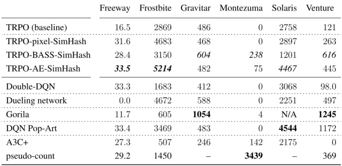
This chapter presents a simple approach for exploration, which extends classic counting-based methods to high-dimensional, continuous state spaces. We discretize the state space with a hash function and apply a bonus based on the state-visitation count. The hash function can be chosen to appropriately balance generalization across states, and distinguishing between states. We select problems from rllab [18] and Atari 2600 [6] featuring sparse rewards, and demonstrate near state-of-the-art performance on several games known to be hard for naïve exploration strategies. The main strength of the presented approach is that it is fast, flexible and complementary to most existing RL algorithms.

In summary, this chapter proposes a generalization of classic count-based exploration to high-dimensional spaces through hashing (Section 3.2); demonstrates its effectiveness on challenging deep RL benchmark problems and analyzes key components of well-designed hash functions (Section 3.4).

3.2

Methodology

Count-Based Exploration via Static Hashing

Our approach discretizes the state space with a hash functionφ : S →_Z. An exploration bonus

r+ _:_{S →}

Ris added to the reward function, defined as

r+(s) = _p β

n(φ(s)), (3.1)

whereβ ∈_R≥0 is the bonus coefficient. Initially the countsn(·)are set to zero for the whole range

ofφ. For every statestencountered at time stept,n(φ(st))is increased by one. The agent is trained

with rewards(r+r+₎_{, while performance is evaluated as the sum of rewards without bonuses.}

Note that our approach is a departure from count-based exploration methods such as MBIE-EB since we use a state-space countn(s)rather than a state-action countn(s, a). State-action counts

n(s, a)are investigated in the Supplementary Material, but no significant performance gains over state counting could be witnessed. A possible reason is that the policy itself is sufficiently random to try most actions at a novel state.

Clearly the performance of this method will strongly depend on the choice of hash functionφ. One important choice we can make regards thegranularityof the discretization: we would like for

(35)

Algorithm 2:Count-based exploration through static hashing, using SimHash

1 Define state preprocessorg :S →_RD

2 (In case of SimHash) InitializeA∈_Rk×D with entries drawn i.i.d. from the standard

Gaussian distributionN(0,1)

3 Initialize a hash table with valuesn(·)≡0 4 foreach iterationj do

5 Collect a set of state-action samples{(s_m, a_m)}M_m₌₀ with policyπ 6 Compute hash codes through any LSH method, e.g., for SimHash,

φ(sm) = sgn(Ag(sm))

7 Update the hash table counts∀m: 0≤m≤M asn(φ(s_m))←n(φ(s_m)) + 1 8 Update the policyπusing rewards

r(sm, am) + √ β n(φ(sm)) M m=0 with any RL algorithm

“distant” states to be be counted separately while “similar” states are merged. If desired, we can incorporate prior knowledge into the choice ofφ, if there would be a set of salient state features which are known to be relevant. A short discussion on this matter is given in the Supplementary Material.

Algorithm 2 summarizes our method. The main idea is to use locality-sensitive hashing (LSH) to convert continuous, high-dimensional data to discrete hash codes. LSH is a popular class of hash functions for querying nearest neighbors based on certain similarity metrics [4]. A computationally efficient type of LSH is SimHash [11], which measures similarity by angular distance. SimHash retrieves a binary code of states ∈ Sas

φ(s) = sgn(Ag(s))∈ {−1,1}k, (3.2) whereg :S →_RD _{is an optional preprocessing function and}_A_{is a}_k_×_D_{matrix with i.i.d. entries}

drawn from a standard Gaussian distribution N(0,1). The value fork controls the granularity: higher values lead to fewer collisions and are thus more likely to distinguish states.

Count-Based Exploration via Learned Hashing

When the MDP states have a complex structure, as is the case with image observations, measuring their similarity directly in pixel space fails to provide the semantic similarity measure one would desire. Previous work in computer vision [62, 15, 114] introduce manually designed feature representations of images that are suitable for semantic tasks including detection and classification. More recent methods learn complex features directly from data by training convolutional neural networks [54, 103, 38]. Considering these results, it may be difficult for a method such as SimHash to cluster states appropriately using only raw pixels.

Therefore, rather than using SimHash, we propose to use an autoencoder (AE) to learn mean-ingful hash codes in one of its hidden layers as a more advanced LSH method. This AE takes as

(36)

Figure

+7

References

Download now ( PDF - 69 Page - 9.79 MB )

Outline

Methodology A Case Study of Montezuma’s Revenge Modular Architecture Training Procedure