Tutorial for the WGCNA package for R I. Network analysis of liver expression data in female mice

(1)

Tutorial for the WGCNA package for R

I. Network analysis of liver expression data in female mice

2.c Dealing with large data sets: block-wise network construction and

module detection

Peter Langfelder and Steve Horvath

November 25, 2014

0 Preliminaries: setting up the R session

Here we assume that a new R session has just been started. We load the WGCNA package, set up basic parameters and load data saved in the first part of the tutorial.

Important note: The code below uses parallel computation where multiple cores are available. This works well when R is run from a terminal or from the Graphical User Interface (GUI) shipped with R itself, but at present it does not workwith RStudio and possibly other third-party R environments. If you use RStudio or other third-party R environments, skip theenableWGCNAThreads()call below.

# Display the current working directory

getwd();

# If necessary, change the path below to the directory where the data files are stored. # "." means current directory. On Windows use a forward slash / instead of the usual \.

workingDir = "."; setwd(workingDir);

# Load the WGCNA package

library(WGCNA)

# The following setting is important, do not omit.

options(stringsAsFactors = FALSE);

# Allow multi-threading within WGCNA. This helps speed up certain calculations. # At present this call is necessary.

# Any error here may be ignored but you may want to update WGCNA if you see one. # Caution: skip this line if you run RStudio or other third-party R environments. # See note above.

enableWGCNAThreads()

(2)

lnames = load(file = "FemaleLiver-01-dataInput.RData");

#The variable lnames contains the names of loaded variables.

lnames

We have loaded the variablesdatExpr anddatTraitscontaining the expression and trait data, respectively.

2 Construction of the gene network and identification of modules

This step is the bedrock of all network analyses using the WGCNA methodology. We present three different ways of constructing a network and identifying modules:

a. Using a convenient 1-step network construction and module detection function, suitable for users wishing to arrive at the result with minimum effort;

b. Step-by-step network construction and module detection for users who would like to experiment with cus-tomized/alternate methods;

c. An automatic block-wise network construction and module detection method for users who wish to analyze data sets too large to be analyzed all in one.

In this tutorial section, we illustrate the automatic block-wise network construction and module detection, suitable for large data sets.

2.c

Automatic block-wise network construction and module detection

2.c.1 Choosing the soft-thresholding power: analysis of network topology

Constructing a weighted gene network entails the choice of the soft thresholding power β to which co-expression similarity is raised to calculate adjacency [1]. The authors of [1] have proposed to choose the soft thresholding power based on the criterion of approximate scale-free topology. We refer the reader to that work for more details; here we illustrate the use of the functionpickSoftThresholdthat performs the analysis of network topology and aids the user in choosing a proper soft-thresholding power. The user chooses a set of candidate powers (the function provides suitable default values), and the function returns a set of network indices that should be inspected, for example as follows:

# Choose a set of soft-thresholding powers

powers = c(c(1:10), seq(from = 12, to=20, by=2))

# Call the network topology analysis function

sft = pickSoftThreshold(datExpr, powerVector = powers, verbose = 5)

# Plot the results:

sizeGrWindow(9, 5) par(mfrow = c(1,2)); cex1 = 0.9;

# Scale-free topology fit index as a function of the soft-thresholding power

plot(sft$fitIndices[,1], -sign(sft$fitIndices[,3])*sft$fitIndices[,2],

xlab="Soft Threshold (power)",ylab="Scale Free Topology Model Fit,signed R^2",type="n", main = paste("Scale independence"));

text(sft$fitIndices[,1], -sign(sft$fitIndices[,3])*sft$fitIndices[,2], labels=powers,cex=cex1,col="red");

# this line corresponds to using an R^2 cut-off of h

abline(h=0.90,col="red")

# Mean connectivity as a function of the soft-thresholding power

plot(sft$fitIndices[,1], sft$fitIndices[,5],

xlab="Soft Threshold (power)",ylab="Mean Connectivity", type="n", main = paste("Mean connectivity"))

text(sft$fitIndices[,1], sft$fitIndices[,5], labels=powers, cex=cex1,col="red")

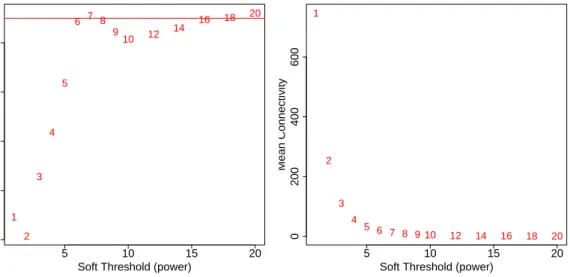
The result is shown in Fig. 1. We choose the power 6, which is the lowest power for which the scale-free topology fit index curve flattens out upon reaching a high value (in this case, roughly 0.90).

(3)

5 10 15 20 0.0 0.2 0.4 0.6 0.8 Scale independence

Soft Threshold (power)

Scale Free Topology Model Fit,signed R^2 1

2 3 4 5 6 7 8 9 10 12 14 16 18 20 5 10 15 20 0 200 400 600 Mean connectivity

Soft Threshold (power)

Mean Connectivity 1 2 3 4 5 6 7 8 9 10 12 14 16 18 20

Figure 1: Analysis of network topology for various soft-thresholding powers. The left panel shows the scale-free fit index (y-axis) as a function of the soft-thresholding power (x-axis). The right panel displays the mean connectivity (degree,y-axis) as a function of the soft-thresholding power (x-axis).

2.c.2 Block-wise network construction and module detection

Throughout this tutorial we work with a relatively small data set of 3600 measured probes. However, modern mi-croarrays measure up to 50,000 probe expression levels at once. Constructing and analyzing networks with such large numbers of nodes is computationally challenging even on a large server. We now illustrate a method, implemented in the WGCNA package, that allows the user to perform a network analysis with such a large number of genes. Instead of actually using a very large data set, we will for simplicity pretend that hardware limitations restrict the number of genes that can be analyzed at once to 2000. The basic idea is to use a two-level clustering. First, we use a fast, computationally inexpensive and relatively crude clustering method to pre-cluster genes into blocks of size close to and not exceeding the maximum of 2000 genes. We then perform a full network analysis in each block separately. At the end, modules whose eigengenes are highly correlated are merged. The advantage of the block-wise approach is a much smaller memory footprint (which is the main problem with large data sets on standard desktop computers), and a significant speed-up of the calculations. The trade-off is that due to using a simpler clustering to obtain blocks, the blocks may not be optimal, causing some outlying genes to be assigned to a different module than they would be in a full network analysis.

We will now pretend that even the relatively small number of genes, 3600, that we have been using here is too large, and the computer we run the analysis on is not capable of handling more than 2000 genes in one block. The automatic network construction and module detection functionblockwiseModulescan handle the splitting into blocks automatically; the user just needs to specify the largest number of genes that can fit in a block:

bwnet = blockwiseModules(datExpr, maxBlockSize = 2000,

power = 6, TOMType = "unsigned", minModuleSize = 30, reassignThreshold = 0, mergeCutHeight = 0.25, numericLabels = TRUE,

saveTOMs = TRUE,

saveTOMFileBase = "femaleMouseTOM-blockwise", verbose = 3)

We have chosen the soft thresholding power 6, a relatively large minimum module size of 30, and a medium sensitivity (deepSplit=2) to cluster splitting. The parametermergeCutHeightis the threshold for merging of modules. We have also instructed the function to return numeric, rather than color, labels for modules, and to save the Topological Overlap Matrix. The output of the function may seem somewhat cryptic, but it is easy to use. For example,

(4)

bwnet$colorscontains the module assignment, andbwnet$MEscontains the module eigengenes of the modules. A word of caution for the readers who would like to adapt this code for their own data. The function blockwiseModules has many parameters, and in this example most of them are left at their default value. We have attempted to provide reasonable default values, but they may not be appropriate for the particular data set the reader wishes to analyze. We encourage the user to read the help file provided within the package in the R envi-ronment and experiment with tweaking the network construction and module detection parameters. The potential reward is, of course, better (biologically more relevant) results of the analysis.

A second word of caution concerning block size. In particular, the parametermaxBlockSizetells the function how large the largest block can be that the reader’s computer can handle. In this example we have set the maximum block size to 2000 to illustrate the block-wise analysis and its results, but this value is needlessly small for most modern computers; the default is 5000 which is appropriate for most modern desktops. If the reader has access to a large workstation with more than 4 GB of memory, the parameter maxBlockSize can be increased. A 16GB workstation should handle up to 20000 probes; a 32GB workstation should handle perhaps 30000. A 4GB standard desktop or a laptop may handle up to 8000-10000 probes, depending on operating system and other running programs. In general it is preferable to analyze a data set in as few blocks as possible.

Below we will compare the results of this analysis to the results of Section 2.a in which all genes were analyzed in a single block. To make the comparison easier, we relabel the block-wise module labels so that modules with a significant overlap with single-block modules have the same label:

# Load the results of single-block analysis

load(file = "FemaleLiver-02-networkConstruction-auto.RData");

# Relabel blockwise modules

bwLabels = matchLabels(bwnet$colors, moduleLabels);

# Convert labels to colors for plotting

bwModuleColors = labels2colors(bwLabels)

To see how many modules were identified and what the module sizes are, one can usetable(bwLabels). Its output is

> table(bwLabels)

0 1 2 3 4 5 6 7 8 9 10 11 12 13 14 15 16 17 18 19

142 472 470 479 271 327 130 209 153 121 100 100 104 77 73 81 40 42 34 91 20

84

and indicates that there are 20 modules, labeled 1 through 20, The label 0 is reserved for genes outside of all modules. The hierarchical clustering dendrograms (trees) used for the module identification for each block are returned inbwnet$dendrograms[[1]], bwnet$dendrograms[[2]]. The dendrograms can be displayed together with the color assignment using the following code:

# open a graphics window

sizeGrWindow(6,6)

# Plot the dendrogram and the module colors underneath for block 1

plotDendroAndColors(bwnet$dendrograms[[1]], bwModuleColors[bwnet$blockGenes[[1]]], "Module colors", main = "Gene dendrogram and module colors in block 1", dendroLabels = FALSE, hang = 0.03,

addGuide = TRUE, guideHang = 0.05)

# Plot the dendrogram and the module colors underneath for block 2

plotDendroAndColors(bwnet$dendrograms[[2]], bwModuleColors[bwnet$blockGenes[[2]]], "Module colors", main = "Gene dendrogram and module colors in block 2", dendroLabels = FALSE, hang = 0.03,

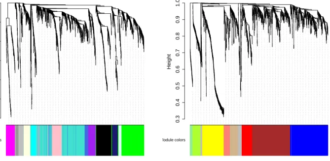
The resulting plots are shown in Fig. 2. We note that if the user would like to change some of the tree cut, module membership, and module merging criteria, the package provides the function recutBlockwiseTrees that can apply modified criteria without having to recompute the network and the clustering dendrogram, thus saving a substantial amount of time.

(5)

0.4 0.5 0.6 0.7 0.8 0.9 1.0

Gene dendrogram and module colors in block 1

Height Module colors 0.3 0.4 0.5 0.6 0.7 0.8 0.9 1.0

Gene dendrogram and module colors in block 2

Height

Module colors

Figure 2: Clustering dendrograms of genes, with dissimilarity based on topological overlap, together with assigned module colors. There is one gene dendrogram per block.

2.c.3 Comparing the single block and block-wise network analysis

We now compare the results of the block-wise analysis with 2 blocks to the results Section 2.a in which all genes were analyzed in a single block. A simple visual check can be obtained by plotting the single-block dendrogram with the single-block and block-wise module colors underneath the dendrogram:

sizeGrWindow(12,9)

plotDendroAndColors(geneTree,

cbind(moduleColors, bwModuleColors), c("Single block", "2 blocks"),

main = "Single block gene dendrogram and module colors", dendroLabels = FALSE, hang = 0.03,

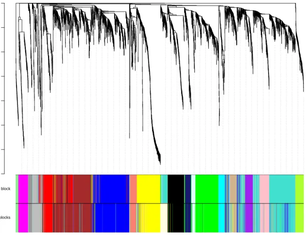
The resulting plot is shown in Fig. 3. Visual inspection confirms that there is excellent agreement between the single-block and the block-wise module assignment.

We now verify that module eigengenes of modules that correspond to one another in the single-block and block-wise approaches are extremely similar. We first calculate the module eigengenes based on the single block and block-wise module colors:

singleBlockMEs = moduleEigengenes(datExpr, moduleColors)$eigengenes; blockwiseMEs = moduleEigengenes(datExpr, bwModuleColors)$eigengenes;

Next we match the single-block and block-wise eigengenes by name and calculate the correlations of the corresponding eigengenes:

single2blockwise = match(names(singleBlockMEs), names(blockwiseMEs)) signif(diag(cor(blockwiseMEs[, single2blockwise], singleBlockMEs)), 3) The result is

> signif(diag(cor(blockwiseMEs[, single2blockwise], singleBlockMEs)), 3)

(6)

0.3 0.4 0.5 0.6 0.7 0.8 0.9 1.0

Single block gene dendrogram and module colors

Height

Single block

2 blocks

Figure 3: Clustering dendrogram of genes obtained in the single-block analysis in Section 2.a, together with module colors determined in the single-block analysis and the module colors determined in the block-wise analysis. There is excellent agreement between the single-block and block-wise network construction and module detection.

1.000 1.000 0.990 1.000 1.000

MEgreenyellow MEgrey MEgrey60 MElightcyan MElightgreen

1.000 0.959 0.999 0.978 1.000

MEmagenta MEmidnightblue MEpink MEpurple MEred

1.000 1.000 0.998 0.999 0.970

MEsalmon MEtan MEturquoise MEyellow

0.997 0.991 -0.991 0.999

Each number above represents the correlation of a single-block eigengene with its corresponding block-wise counter-part. The correlations are all very close to 1 (the turquoise eigengene changed orientation), again indicating that the block-wise and single-block analyses lead to very similar results.

References

[1] B. Zhang and S. Horvath. A general framework for weighted gene co-expression network analysis. Statistical Applications in Genetics and Molecular Biology, 4(1):Article 17, 2005.

Tutorial for the WGCNA package for R I. Network analysis of liver expression data in female mice