Optimization of Boolean Expressions
for Main Memory Database Systems
Inauguraldissertation
zur Erlangung des akademischen Grades
eines Doktors der Naturwissenschaften
der Universit¨
at Mannheim
vorgelegt von
Fisnik Kastrati, M.Sc.
aus Pristina
Korreferent: Professor Dr. Christian Becker, Universit¨at Mannheim
Acknowledgments
First and foremost, I would like to express my deepest appreciation to my advisor prof. Guido Moerkotte. His guidance and supervision has enabled me to grow as a researcher, as well as become a better computer scientist in general. His immense knowledge in the area of query optimisation and databases has proved invaluable to me throughout my entire PhD journey. A special thank you goes to my second advisor prof. Christian Becker for reviewing my thesis and serving in my thesis committee.
I would like to thank Simone Seeger for her meticulous proofreading of my draft papers. Im grateful to my colleagues Marius Eich and Magnus M¨uller for their feedback and comments.
I would also like to acknowledge University of Mannheim for the dissertation completion grant (Landesgraduiertenf¨orderung – LGF) which had removed the financial burden during my thesis writing.
Last but not least, I would like to thank my wife for her love, support and constant encouragement. Many thanks go as well to my parents who were very supportive throughout my PhD.
Abstract
With the ubiquity of main memory databases which are increasingly replac-ing the old disk-oriented databases, relations are bereplac-ing stored in denormalized form in order to increase the query throughput, thus, the dominance of join operators in terms of costs is being replaced by the costs of evaluating selec-tion predicates. Boolean expressions containing selecselec-tion predicates connected both conjunctively and disjunctively have been thus far solved by rather simple heuristics which leaves a large optimization potential unharvested. To exacer-bate the matter, such heuristics rely on the independent predicate selectivity assumption which typically does not hold, and the constant predicate costs assumption which in terms of main memory database systems does not hold ei-ther. In this thesis we tackle the problem of optimizing Boolean expressions by not relying on the independence assumption nor the constant predicate costs assumption. We present optimization algorithms for queries containing both conjunctively and disjunctively connected predicates together with a cost model which precisely captures CPU architectural characteristics such as branch mis-prediction. Our optimization algorithms achieve the optimum in terms of plan quality, thus, they harvest the entire optimization potential inherent in Boolean expressions.
Zusammenfassung
Die sich wandelnde Hardwarelandschaft f¨uhrt dazu, dass Hauptspeicher-Daten-banksysteme die klassischen disk-basierten Systeme zunehmend verdr¨angen. Hauptspeicher-Datenbanksysteme speichern Relationen in denormalisierter Fo-rm um den Durchsatz an Anfragen zu erh¨ohen. In Folge dessen ¨ubernehmen Selektionspr¨adikate die Rolle von Joins als entscheidenden Kostenfaktor. Kon-junktiv sowie disKon-junktiv verkn¨upfte Boolesche Ausdr¨ucke, welche Selektion-spr¨adikate enthalten, wurden bisher von simplen Heuristiken optimiert. Dies hat viel Spielraum f¨ur Optimierungen gelassen. Die kritischen Schwachstellen dieser Heuristiken sind, dass sie sowohl annehmen, dass die Selektivt¨aten Un-abh¨angigkeit voneinander sind, welches im Allgemeinen nicht gilt, sowie, dass die Evaluationskosten von Pr¨adikaten unempfindlich gegen¨uber ihrer Selek-tivit¨at sind. Letzteres spiegelt insbesondere in Hauptspeicher-Datenbanksys-temen die Realit¨at nicht wider. Diese Arbeit behandelt die Optimierung von Booleschen Ausdr¨ucken ohne diese Annahmen. Wir zeigen Optimierungsalgo-rithmen f¨ur Anfragen, die sowohl konjunktiv als auch disjunktiv verkn¨upfte Pr¨adikate enthalten. Dar¨uber hinaus pr¨asentieren wir ein daf¨ur angepasstes Kostenmodell, welches Charakteristiken der Prozessorarchitektur, wie branch misprediction, pr¨azise modelliert. Unsere Optimierungsalgorithmen sind opti-mal in Bezug auf die Planqualit¨at; sie sch¨opfen das gesamte Optimierungspo-tential Boolescher Ausdr¨ucke aus.
Contents
1. Introduction 15
2. Preliminaries 17
2.1. Relational Model . . . 17
2.2. Computer Architecture . . . 19
2.2.1. Instruction Pipelining in Modern Processors . . . 19
2.2.2. Branch Misprediction . . . 20
2.2.3. Hierarchical Organization of Memory . . . 23
2.2.4. Virtual Memory . . . 24
2.2.5. Translation Lookaside Buffer . . . 26
2.3. Storage Layouts for a Main Memory Database System . . . 26
2.3.1. Row Stores - NSM Layout . . . 27
2.3.2. Column Stores - DSM Layout . . . 27
2.4. Iterator Model . . . 30
3. SystemTx 35 3.1. Introduction . . . 35
3.1.1. Physical operators in SystemTx . . . 36
3.2. A Bad Storage Layout . . . 37
3.3. Storage Layout in SystemTx . . . 39
4. Cost Estimation and Approximation 43 4.1. Introduction . . . 43
4.2. Related Work . . . 44
4.3. The Convex Paranorm: Q-paranorm . . . 45
4.4. The Link between Q-Error and Plan Quality . . . 47
4.5. Cost Model . . . 49
4.5.1. Cost Functions . . . 51
4.5.2. Memory Access Costs . . . 54
4.5.3. Branch Misprediction Costs . . . 55
4.6. Approximation of Cost Functions . . . 57
4.6.1. Application in SystemTx . . . 60
4.7. Cost Model Validation . . . 60
5. Optimization of Conjunctive Predicates 63 5.1. Introduction . . . 63
5.2. Related Work . . . 65
5.3. TheDPSel Optimization Algorithm for Conjunctive Predicates 66 5.4. Evaluation . . . 70
5.4.1. General Case . . . 71
5.4.3. TPC-H Dataset . . . 74
5.4.4. Forest Dataset . . . 75
5.4.5. Plan Quality Loss in Presence of Cardinality Estimation Errors . . . 75
5.4.6. Runtime . . . 76
5.5. Conclusion . . . 77
6. A Heuristic for Boolean Expressions 79 6.1. Introduction . . . 79
6.2. Related Work . . . 82
6.3. Preliminaries . . . 84
6.3.1. Predicates . . . 84
6.4. Plan Construction Strategies . . . 85
6.4.1. Traditional Plans: DNF and CNF . . . 86
6.4.2. Bypass Plans . . . 86
6.5. A Heuristic Optimization Algorithm for Boolean Expressions . . 87
6.5.1. Overview of the Algorithm . . . 87
6.5.2. The Algorithm in Detail . . . 89
6.5.3. Optimization of Conjunctive Predicates in Boolean Sum-mands . . . 92
6.6. Evaluation of the Heuristic Algorithm . . . 94
6.6.1. Forest Dataset . . . 95
6.6.2. Predicates with Random Selectivities . . . 100
6.6.3. CH-benchmark . . . 103
6.6.4. Runtime . . . 104
6.7. Conclusion . . . 105
7. Optimal Evaluation of Boolean Expressions 107 7.1. Introduction . . . 107
7.2. The Optimization Algorithm . . . 108
7.2.1. The Basic Idea . . . 109
7.2.2. The Algorithm in Detail . . . 109
7.2.3. Memoization . . . 111
7.2.4. Branch-and-bound Pruning . . . 112
7.2.5. Accumulated-Cost Bounding . . . 113
7.2.6. Predicted-Cost Bounding . . . 116
7.2.7. Boolean Implications . . . 116
7.3. Boolean Difference Calculus . . . 117
7.4. Boolean Expression Implementation . . . 117
7.5. Evaluation . . . 119
7.5.1. Forest dataset . . . 120
7.5.2. Runtime of Top-Down Algorithms . . . 120
7.5.3. Evaluation of two heuristics . . . 123
7.5.4. Optimization Potential . . . 126
7.5.5. Runtime . . . 127
7.5.6. CH-benchmark . . . 127
Contents 7.5.8. Weather Dataset . . . 130 7.6. Conclusion . . . 130 7.6.1. Graceful Degradation . . . 132
8. Cardinality Estimation 133
8.1. Cardinality Estimation based on Sampling . . . 133 8.2. Cardinality Estimation for Conjunctive Predicates . . . 135 8.3. Cardinality Estimation for Disjunctive Predicates . . . 136
9. Conclusion 139
A. Implementation Details 141
A.1. Allocator in SystemTx . . . 141 A.1.1. Chunk-wise Column Organization in SystemTx . . . 142
List of Figures
2.1. Illustration of sequential execution and instruction pipelining in
a five stage RISC processor . . . 19
2.2. Illustration of a pipeline stall . . . 20
2.3. Memory organization in a Intel i7-4770 Haswell processor . . . . 23
2.4. Illustration of the contiguous virtual memory on the left and its mapping into the physical memory and the disk on the right . . . 25
2.5. Vertical partitioning of the Movies relation . . . 28
2.6. Scan time in a row store and a column store over a single attribute 29 2.7. An UML graph of physical operators in SystemTx . . . 30
2.8. Illustration of the pull-based iterator model . . . 31
2.9. Illustration of tuple processing schemes. The x-axis denotes the vector size. Figure taken from [65]. . . 33
3.1. Column access costs over the initial storage layout . . . 37
3.2. The effect of DTLB misses on a column store . . . 38
3.3. The effect of DTLB misses on a column store . . . 39
3.4. Illustration of the chunk-wise storage layout in SystemTx . . . . 40
3.5. Reduced DTLB miss effect using the new storage layout . . . 41
3.6. Reduced DTLB miss effect using the new storage layout . . . 41
3.7. Reduced DTLB miss effect using the new storage layout . . . 42
4.1. Plan types . . . 51
4.2. Plan types for measuring the costs of the dereference operator . . 54
4.3. SystemTx: column access costs . . . 54
4.4. Q-error of dereferenciation . . . 55
4.5. Execution time of a selection operator . . . 55
4.6. Approximation of branch misprediction penalty . . . 57
5.1. Pseudocode forBuildPlans . . . 67
5.2. Pseudocode forDPSel . . . 67
5.3. Pseudocode forStoreSolution . . . 67
5.4. Dependency graph for the example query . . . 68
5.5. A bitvector of integral typeuint32 t representing a set of predi-catesP ={1,2,4,7,8} . . . 70
5.6. Plan costs for inexpensive predicates sharing a single subexpression 72 5.7. Plan costs for inexpensive predicates, no shared subexpression . . 73
5.8. Plan costs for inexpensive predicates depending on 3 different subexpressions . . . 74
5.9. The evaluation results of runtime performance . . . 77
6.2. Evaluation plans for the query (Pc∧Pl)∨Pr . . . 85
6.3. Bypass plan construction for the example query (x1∧x2∧x3)∨ (x2∧x5∧x6) . . . 88
6.4. Pseudocode forBypassPlanGen . . . 89
6.5. Pseudocode forOptimize . . . 89
6.6. Pseudocode forDPSel . . . 90
6.7. Pseudocode forBuildPlans . . . 90
6.8. Pseudocode forStoreSolution . . . 90
6.9. Dependency graph for the example query . . . 93
6.10. Illustration of building bypass plans . . . 93
6.11. The evaluation results of runtime performance . . . 104
7.1. Pseudocode forTDsim. . . 109
7.2. Predicate assignment and Boolean expression simplification . . . 110
7.3. Pseudocode forTDmemo . . . 111
7.4. Pseudocode forTDacb . . . 114
7.5. Pseudocode forBDC. . . 118
7.6. Tree representation of the expression (x1∧x2)∨(x1∧x3)∨(x1∧x4)118 8.1. An example bypass plan for expression (p1∧p2)∨p3 . . . 136
List of Tables
2.1. Movies relation . . . 17
2.2. Memory access times in a Intel i7-4770 Haswell processor . . . . 23
4.1. Equations for approximating a set of numbers and the error they minimize . . . 46
4.2. Attributes and their contents for the test relation R . . . 50
4.3. Notation . . . 52
4.4. Cost functions . . . 52
4.5. True vs. estimated costs . . . 61
5.1. Overview of related work . . . 66
5.2. Relative optimization potential (in factors!) of DPSelvs. Rank and Selfor the range of predicates 3-6. . . 71
5.3. Relative optimization potential (in factors!) of DPSelvs. Rank and Selfor the range of predicates 7-10. . . 71
5.4. DPSelvs. Rankand Selover TPC-H dataset . . . 74
5.5. Relative optimization potential of DPSel vs. Rank and Sel over the Forest dataset . . . 75
5.6. The max q-error between ebest and eopt for different f values . . 76
6.1. Overview of related work . . . 84
6.2. Relative optimization potential (in factors!) of BypassPlan-Genvs. DNFalg,DNFdpand CNFalgover the Forest dataset 96 6.3. Relative optimization potential (in factors!) of BypassPlan-Genvs. DNFalg,DNFdpand CNFalgover the Forest dataset 96 6.4. Average time-per-tuple (ns) for query plans over the Forest dataset 96 6.5. Average time-per-tuple (ns) for query plans over the Forest dataset 96 6.6. Relative optimization potential (in factors!) of BypassPlan-Genvs. DNFalg,DNFdpandCNFalgover the Forest dataset (common predicates) . . . 99
6.7. Average time-per-tuple (ns) for query plans over the Forest dataset (common predicates) . . . 99
6.8. Relative optimization potential ofBypassPlanGenvs. DNFalg, DNFdpand CNFalg, joint predicate selectivities generated by ME principle . . . 101
6.9. Average time-per-tuple (ns), joint predicate selectivities gener-ated by ME principle . . . 101
6.10. Relative optimization potential ofBypassPlanGenvs. DNFalg, DNFdpand CNFalg, joint predicate selectivities generated by ME principle (common predicates) . . . 102
6.11. Average time-per-tuple (ns), joint predicate selectivities
gener-ated by ME principle (common predicates) . . . 102
6.12. CH-benchmark results for Query 19 . . . 104
7.1. Tree vs. bitvector representation (runtimes in ms) . . . 119
7.2. Performance (in ms) for CNF query type (p1∨p2)∧. . . 121
7.3. Performance (in ms) for DNF query type (p1∧p2)∨. . . 121
7.4. Performance (in ms) for CNF query type (p1∨p2∨p3)∧. . . 122
7.5. Performance (in ms) for DNF query type (p1∧p2∧p3)∨. . . 122
7.6. Performance of the heuristics against the optimum for the Forest dataset for DNF queries: (p1∧p2)∨. . . 124
7.7. Performance of the heuristics against the optimum for the Forest dataset for CNF queries: (p1∨p2)∧. . . 124
7.8. Performance of the heuristics against the optimum for the Forest dataset for DNF queries: (p1∧p2∧p3)∨. . . 124
7.9. Performance of the heuristics against the optimum for the Forest dataset for CNF queries: (p1∨p2∨p3)∧. . . 125
7.10. Runtimes for DNF queries (in ms) . . . 127
7.11. Runtimes for CNF queries (in ms) . . . 127
7.12. CH-benchmark results for Query 19 . . . 128
7.13. The effect of Boolean implications on CNF queries . . . 129
7.14. The effect of Boolean implications on DNF queries . . . 129
7.15. Performance of the heuristics against the optimum for the Weather dataset for DNF queries: (p1∧p2)∨. . . 130
7.16. Performance of the heuristics against the optimum for the Weather dataset for CNF queries: (p1∨p2)∧. . . 131
7.17. Performance of the heuristics against the optimum for the Weather dataset for DNF queries: (p1∧p2∧p3)∨. . . 131
7.18. Performance of the heuristics against the optimum for the Forest dataset for CNF queries: (p1∨p2∨p3)∧. . . 131
8.1. Sample data taken from the Forest [14] dataset . . . 134
1. Introduction
Optimization of Boolean expressions in database system is a very challenging problem, which prompts for carefully designed optimization algorithms in order to harvest the large optimization potential inherent in them. With the advent of main memory databases, optimization of Boolean expressions becomes an even more challenging task requiring optimization algorithms which take into account hardware characteristics such as CPU branch misprediction. In the recent years, the memory price has drastically decreased and at the same time its size has drastically increased. For instance, in early 80s the cost per MB of main memory was around 6400 USD, whereas at the time of this thesis writing it is 0.0059 USD1. Servers with terabytes of main memory have now become affordable thus prompting a shift from disk oriented database systems to main memory oriented database systems. Consequently, this thesis focuses on optimization of Boolean expressions for main memory databases.
In the first part of this thesis, we consider the problem of optimizing Boolean expressions composed of predicates connected conjunctively. We present an efficient optimization algorithm for this class of queries which relies on dynamic programming and generates the solutions in a bottom-up fashion.
Boolean expressions containing predicates connected conjunctively and dis-junctively are then the topic of the second and the third part of this thesis. We initially present an efficient heuristic optimization algorithm for disjunctive predicates which leverages bypass processing. Although the heuristic algorithm is superior to the existing heuristics in the literature, it does not attain the optimum in terms of plan quality. We can, however, achieve the optimum by means of the optimization algorithm presented in the third part of this thesis, which optimizes Boolean expressions in a top-down fashion. Top-down algo-rithms in contrast to bottom-up algorithm have the advantage of employing search strategies like branch-and-bound pruning in order to reduce the search space. Besides the branch-and-bound pruning search strategy, our top-down optimization algorithms make a use of the Boolean difference calculus in order to derive tighter upper bounds and this way prune even more aggressively the search space.
Optimization algorithms found in the literature—and commonly used in com-mercial relational database systems—rely on at least two assumptions: (1) pred-icate selectivities are assumed to be independent, and (2) predpred-icate costs are assumed to be constant. Since both of these two assumptions typically do not hold, optimization algorithms presented in this thesis do not rely on any of them. Since we do not rely on the independence assumption, in the fourth part of this thesis we present a very efficient sampling method, which can be used to
1
gather predicate selectivities for all the subsets of predicates given in a query. To that end, optimization algorithms presented in this thesis work take into consideration CPU architectural characteristics such as branch misprediction penalty, as well as common subexpression elimination when present in Boolean expressions.
Since the cost model plays a principal role in query optimization, we present a cost model which very precisely models hardware characteristics such as branch misprediction penalty as well as cache misses. The cost model presented in this thesis is novel in that it shows a direct relationship between the error in the cost functions and the plan quality.
The rest of the thesis is organized as follows. In Chapter 2 we presented the preliminaries required to understand the subsequent chapters. Chapter 3 presents the system prototype used in this work. The cost model used in our optimization algorithms is presented in Chapter 4 together with the approxima-tion framework which is used to obtain the parameters for our cost funcapproxima-tions. The optimization algorithm for conjunctive Boolean expressions is the topic of Chapter 5. A heuristic for Boolean expressions containing both conjunc-tive and disjuncconjunc-tive predicates is presented in Chapter 6. Chapter 7 presents a top-down optimization algorithm for Boolean expressions which attains the optimum in terms of plan quality. Chapter 8 presents a sampling method which efficiently gathers predicate selectivities. Furthermore, in Chapter 8 we show how the predicate selectivities gathered by our sampling method can be used when optimizing queries containing both conjunctive and disjunctive predicates. Finally, Chapter 9 concludes the thesis.
2. Preliminaries
In this chapter we present the preliminaries required to understand the work in this thesis.
Initially we give a brief introduction to the algebra, followed by some back-ground information about the computer architecture. We conclude this chapter by presenting details on the two major materialization strategies used in main memory database systems.
2.1. Relational Model
The relational model was first introduced in 1969 by Edgar F. Codd, and since then it became the de facto standard for data representation in the database community. The relational model is quite pragmatic due to its fundamental building block: mathematical relation. The roots of the relational model come from set theory and first-order predicate logic.
In the relational model, a database is represented as a set of relations. A relation consists of set tuples where each tuple is composed of a number of <attribute, value>pairs. Tuples in a relation represent facts about some entity, or relationships. Relations can be informally thought of as two-dimensional tablesconsisting ofrows andcolumns. Rows represent tuples, whereas columns represent attribute values drawn from a finite domain.
Movie Year IMDb rating
The Godfather 1972 9.2 The Dark Knight 2008 8.9
Pulp Fiction 1994 8.9
A Beautiful Mind 2001 8.2 Table 2.1.: Movies relation
An example relation about movies has been depicted in Table 2.1. This relation describes the movie title, the year when the movie first appeared, and its IMDb1 rating.
The data-manipulation part of the relational model is defined in relational algebra. The relational algebra operators are divided into two groups. The first group include set operators coming from mathematical set theory. Such operators are set union (∪), set difference (∩), set intersection (\) and cross product (×). Since in relational model relations are defined as a set of tuples, the above enumerated set operators are applicable. If, however, duplicates are
1
to be considered, then we denote with (∪-) the union operator without duplicate
elimination.
ei∪ej :={t|t∈ei∨t∈ej} ei∩ej :={t|t∈ei∧t∈ej} ei\ej :={t|t∈ei∧t /∈ej}
The second group consists of the operators which were developed for rela-tional databases. In the second group belong operators such as selection (σ), projection (π), join (./) among others.
The selection operator filters out all the tuples that do not satisfy the predi-cate p:
σp(e) :={t|t∈e∧p(e)}.
We make no restriction on the predicatep, it can include method calls, nested expressions, etc. Further, if the input of the selection does not contain duplicate values, the output is duplicate-free too.
The projection operatorπ can be used to remove attributes πA(e) :={a1:x.a1, . . . , an:x.an|x∈e}
whereas the operator which is used to create (compute) new attributes is the map operator χ [4, 44]: χA1:e0
1,...,Ak:e0k(e). The map operator extends an input
tuple by a new attributeA, whose value is calculated via an arbitrary expression e0:
χA:e0(e) :={t◦[A:v]|t∈e, v=e0(t)},
where ◦ denotes the tuple concatenation operator. We generalize the map operator for many attributes as follows:
χA1:e01,...,Ak:e0k(e) :=χAk:e0k(. . . χA1:e01(e). . .).
In relational algebra there exists many variants of join operators. Five of them are rather standard and encountered often in the literature. These are join, semijoin, antijoin, left outerjoin, and full outerjoin. We will only give the definition for the cross product and the regular join operator:
ei×ej :={x◦y|x∈ei∧y∈ej}
ei ./p ej :={x◦y|x∈ei∧y∈ej∧p(x, y)}, the definitions for the rest of join operators can be found in [46].
The input to relational algebra operators are instances of relations, and the result of algebra operators are new relations. The newly produced relations can be an input to other operators and this way one can flexibly combine a sequence of relational algebra operations in a relational algebra expression. To this end, relational algebra expressions enable users to specify their information retrieval requests. As an example, lets assume that we are interested in finding all the movie names that appeared in the time period between 1990 and 2005 from the
2.2. Computer Architecture movies relation depicted in Figure 2.5. This retrieval request can be expressed in relational algebra as follows:
πmovie(σyear≥1990∧year≤2005(M ovies)).
Relational algebra is less expressive than conventional programming lan-guages such as C++, Java, etc. That is, there are computations possible in programming languages which cannot be performed in relational algebra. How-ever, limitations in its expressive power make relational algebra easier to write queries in, and further, they allow the optimizer to generate a highly optimized code.
2.2. Computer Architecture
In the following subsections, we present computer architectural details which are of relevance to understanding the material presented later. The material touching the hardware covers only background information for readers not fa-miliar with the modern computer architecture and is by no means exhaustive. Readers interested in more details about the computer architecture are referred to the excellent book by David A. Patterson and John LeRoy Hennessy – “Com-puter Architecture: A Quantitative Approach” [27].
2.2.1. Instruction Pipelining in Modern Processors
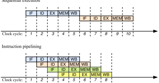
Figure 2.1.: Illustration of sequential execution and instruction pipelining in a five stage RISC processor
Execution in a processor is typically broken into a number of stages, where specialized processor units execute each stage. In the most basic computing model, the processor executes at most one instruction per clock cycle, this way only one execution unit is active at any clock cycle while other execution units
Figure 2.2.: Illustration of a pipeline stall
remain idle. This model is known as the sequential execution model. Modern processors, however, allow for more than a single instruction to be executed concurrently at any given clock cycle in order to increase the throughput. This computation model is known as instruction pipelining, or instruction-level par-allelism.
Execution stages in a processor typically follow the pattern: instruction fetch (IF), instruction decode (ID), instruction execute (EX), memory access (MEM), and write back (WB), i.e., save the results in a register (if necessary). The MEM stage is applicable only when the instruction needs to access the data memory. The difference between a pipelined execution model and the sequential one has been illustrated in Figure 2.1. Note that modern CPUs have more stages than the ones shown in this illustration, e.g., Intel Haswell processor has a 14-stage pipeline and on the other extreme, Intel Prescott processor has a 31-14-stage pipeline.
2.2.2. Branch Misprediction
For a program without conditional statements, the code is simply a sequence of instructions allowing for a pipelined execution as shown in the bottom part of Figure 2.1. If the program, however, contains conditional statements, CPU tries to predict the outcome of the predicate and load into the pipeline in-structions corresponding to the predicted execution path. This happens as the CPU cannot support simultaneously all the possible paths in pipelined execu-tion, therefore it has to guess the execution path. If the guessed execution path turns out to be wrong, then several instruction in the pipeline have to be flushed, thus causing apipeline stall.
Figure 2.2 illustrates the branch misprediction and the resulting pipeline stall. Assume that instruction 2 in the illustration is a conditional statement, and hence at clock cycle 3, the processor speculatively fetches instruction 3 and as a result, it executes the wrong sequence of the instructions 4,5, and 6. When instruction 2 is completely executed at clock cycle 6, the CPU detects that the sequence of the instructions 3-6 are wrongly executed, therefore it flushes the pipeline and in clock 7 starts loading the correct sequence of the instructions
2.2. Computer Architecture 7-10. When the instruction 7 is being fetched (IF), there is no overlapping with earlier instructions due to the pipeline being flushed, and therefore CPU resources are wasted. That is, the branch misprediction has delayed (stalled) the execution of the instruction 7 by 4 cycles, whereas the normal delay between two instructions is only 1 cycle, e.g., see the execution of the instructions 1 and 2 in Figure 2.2.
In real processors, delays due to control hazards like branch misprediction are much longer as there the number of pipeline stages is larger. In Intel i7-4770 Haswell processor the branch misprediction penalty is quite severe— it costs 18-20 cycles2, which makes the optimization of this penalty critical. The optimization algorithms presented in Chapter 5, Chapter 6 and Chapter 7 judicially optimize this penalty in the context of main memory databases.
Branching and Non-branching Conditions
As mentioned in the previous section, the presence of conditional statements in a program can cause control-hazards due to branch misprediction(s). A conditional statement can be composed of multiple predicates connected con-junctively. Consider the following simple expression containing a conjunction p1∧p2 of predicates. This conditional statement in programming languages like C/C++ can be evaluated by expressions either of the form p1&&p2 or of the formp1&p2. The evaluation of&is performed by first evaluating both its argu-ments. Then, thelogical and (∧) is calculated by abitwise and operation. The expression p1&&p2 is evaluated by first evaluating p1. If p1 evaluates to false, this is the result. If p1 evaluates to true, then and only then p2 is evaluated. The result of this evaluation is the result of the whole expression. To that end, the evaluation of the expression p1&&p2 includes a conditional branch, which introduces a possibility for branch misprediction. The evaluation of the expres-sionp1&p2 does not include a conditional branch, although after its evaluation there might be one.
To better understand the branching AND (&&) and non-branching AND (&) logical connections, let us consider the following simple C/C++ code snippet: bool branchingAnd (i n t p1 , i n t p2 ) { i f( p1 > c1 && p2 < c2 ) { return true; } return f a l s e; } bool nonbranchingAnd (i n t p1 , i n t p2 ) { i f( p1 > c1 & p2 < c2 ) { return true; } return f a l s e; } 2 http://www.7-cpu.com/cpu/Haswell.html
The first functionbranchingAnd(int p1, int p2)contains an if condition with the branching AND (&&) connection, whereas the second function contains
the same condition, however, with a non-branching AND (&) connection. In the following, we show the assembly code generated when compiling these two functions using Intel’s C++ compiler (icpc version 16.0.3):
1 branchingAnd ( i n t , i n t ) : 2 cmp e d i , DWORD PTR c1 3 j l e . . B1 . 4 4 cmp e s i , DWORD PTR c2 5 jge . . B1 . 4 6 mov eax , 1 7 r e t 8 . . B1 . 4 :
9 xor eax , eax
10 r e t
11
12 nonbranchingAnd ( i n t , i n t ) :
13 xor eax , eax
14 mov r8d , 1
15 xor edx , edx
16 cmp e d i , DWORD PTR c1
17 cmovg edx , r8d
18 xor ecx , ecx
19 cmp e s i , DWORD PTR c2
20 cmovl ecx , r8d
21 t e s t edx , ecx
22 cmovne eax , r8d
23 r e t
For the branchingAnd(int p1, int p2)function, the compiler has
gener-ated a conditional jump to location ..B1.4 if the condition p1 > c1 is not satisfied, as shown in line 3. In such case, the second condition is bypassed altogether and the function returns a false value. In the generated code, how-ever, there is also a second conditional jump shown in line 5. The second jump corresponds to the second condition (p2 < c2), and is taken only if the first condition succeeds, but the second one fails.
For thenonbranchingAnd(int p1, int p2)function, there are no such con-ditional jumps in the generated assembly code. Both conditions are evaluated, and their results are stored in the registers edx, and ecx. These two registers
will hold binary values (1 or 0) depending on the outcome of the respective con-ditions. In line 21, however, there is a bitwise test instruction, which performs a bitwise-AND over the registers edx, andesx. If the bitwise test yields 1, the
C/C++ code inside the if statement will be executed, otherwise the code control will return to the point outside the if statement, that is, our function will return false. To this end, depending on the predicate selectivities, one should carefully choose either evaluation method in order to minimize the branch misprediction penalty. We present in Chapter 5 an optimization algorithm for conjunctive predicate, which judiciously chooses either logical connection (&&or&)
depend-ing on predicate selectivities in order to minimize the branch misprediction penalty.
2.2. Computer Architecture
Memory Size Latency
registers <1 KB 1-2 cycles L1 cache 64 KB 4 cycles L2 cache 256 KB 12 cycles
L3 cache 8 MB 36 cycles
main memory GB to TB 50 - 200 cycles
Table 2.2.: Memory access times in a Intel i7-4770 Haswell processor
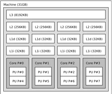
Figure 2.3.: Memory organization in a Intel i7-4770 Haswell processor
2.2.3. Hierarchical Organization of Memory
The gap in performance between processor and main memory started from early 80s to widen deeply in favor of processors. Since the processor speed is much faster than the memory access time, the processor would spend most of the time idle when requesting data from main memory (DRAM). In order to solve this problem, computer architects introduced cache memories between the CPU and the main memory. Caches are small memory pools built using static-RAM (SRAM) technology, thus have very low access times but they are also very expensive.
Since cache memory is expensive it is organized hierarchically. Lower level cache (closer to the CPU) is faster, but smaller and more expensive than the cache(s) situated in higher level(s). The size as well as the latency overhead of the hierarchical memory system in a modern processor is shown in Table 2.2.
Note that L1, L2 caches are typically located on the CPU die while L3 is placed on the system board as it is shared between the CPU cores in a multi-core processor. Further, L1 cache is typically divided for data (L1d) and instructions (L1i). An illustration depicting the hierarchical memory organization in a multi-core processor is shown in Figure 2.3.
Caches work adhering to thetemporal locality principle[27], which means that caches hold the most recently accessed data. The programs are more likely to access again the recently accessed data, and due to the temporal locality principle, the data will be quickly found in the cache and this way resulting in a cache hit. If otherwise, a cache miss occurs and the data item has to be brought-in from the memory (DRAM). More specifically, the CPU will first look-up for a word in the L1 cache, and if not found, it continues searching in the L2 cache, and if not there, it looks it up in the L3 cache and finally in the main memory (DRAM). Each transition of the search from one level to another (deeper) level of memory induces significantly higher look-up costs, as shown in Table 2.2. Programs should therefore be designed with the memory hierarchy in mind in order to minimize the expensive memory traffic between the CPU and DRAM.
For efficiency reasons, the unit of transfer between the cache and the memory is a block or a cache line at the time. The block is typically 64 bytes long (a sequence of words) and in an event of a cache miss, a block of 64 bytes is transfered from memory (or a higher level cache) into the cache. There are three different placement schemes when it comes to placing a block into the cache thus leading to the notion ofcache associativity:
• n-way set associative cache is divided into sets, where set is a group of n blocks of memory (or cache lines). A cache line is first mapped to a set, and then within the set it can be placed anywhere. In order to find a cache line in the cache, the set where the cache line could belong to is first computed, and within the set it is searched for the cache line in parallel. The set is found according to the address of the data [27]:
(cache line address) mod (number of sets in cache),
• direct mapping cache contains sets able to hold only one cache line, there-fore a cache line is always placed in the same location within a set,
• fully associative cache contains only one set, thus a cache line can be placed anywhere within the cache.
2.2.4. Virtual Memory
It is rather inefficient to allocate the entire memory space for each process as many processes use only a portion of their allocated address space. The problem of sharing the physical memory among processes is handled by the operating system by means of the virtual memory.
Virtual memory divides the physical memory intopages and allocates them to each running process. Such an allocation scheme provides protection; each
2.2. Computer Architecture
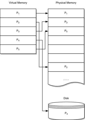
Figure 2.4.: Illustration of the contiguous virtual memory on the left and its mapping into the physical memory and the disk on the right
process can operate only over its allocated space and it cannot access the address space allocated to other processes. Further, by means of the virtual memory, the operating system can assign to processes more virtual memory than the available physical memory. In the sight of the process its assigned (virtual) memory is contiguous, but in reality its (virtual) memory space can be mapped to pages scattered across different locations in the main memory including the disk as well. Figure 2.4 illustrates the mapping of the virtual address space to the physical address. The page size depends on the processor architecture and is typically set to 4 KB, but larger pages are also supported.
Besides managing the physical memory and protection of the address space, virtual memory offers another benefit, it allows loading the same program on any physical memory location by means ofrelocation [27]. That is, the physical memory of a program can be placed anywhere in the main memory or disk and only the mapping of the virtual address space to physical memory need to be updated.
Virtual memory as seen by the process needs to be translated into the physical memory which is used by the hardware. This job is handled by the operating system by utilizing a data structure known as page table. That is, page table allows for translating virtual addresses to physical addresses. Since accessing
the page table for each translation request is an expensive operation, there exists special cache memory dedicated for holding entries of this structure, calledtranslation lookaside buffer (TLB). Details on this structure are given in the following subsection.
2.2.5. Translation Lookaside Buffer
Page tables are typically very large and therefore stored in main memory. A request to translate a virtual memory address to physical memory address takes two memory accesses. The first one is to query the page table (a process called page walk) and the second one to access the actual data. In order to spare the traffic to main memory, most recent address translations are kept in a special cache called translation lookaside buffer (TLB). Just like the regular cache, the TLB is also hierarchical (L1, L2, L3), and divided for data (D-TLB) and instructions (I-TLB).
If the entry for an address translation request cannot be found in the TLB, an event known as TLBmiss occurs. The TLB miss event triggers a page table lookup which is an expensive operation as it amounts to reading a number of memory locations in the page table in order to determine the physical address required by the process. Once the physical address is determined, it is then stored in the TLB, such that future memory translation requests result with a “TLB hit” and this way the expensive page lookups are avoided.
TLB is a very scarce resource, e.g., in Intel Haswell i7-4770 processor, L1 TLB has a capacity of only 64 entries and is 4-way set associative. Further, L1 TLB is split into the TLB for program addresses (I-TLB) and for data addresses (D-TLB). That is, the D-TLB and I-TLB have a capacity of only 32 entries each. Such a small L1 TLB capacity means that the new incoming translation requests if not present in the TLB evict older entries—as in TLB are kept only the most recent entries, according to the temporal locality principle—and this way causing expensive page lookups. Further, equally aligned addresses may also cause expensive page lookups as theymutually evict entries of one another in the TLB, even if the TLB capacity is not exhausted. This is due to the limited associativity typically found in TLBs. We show in Chapter 3 how the mutual eviction of equally aligned addresses affect a column store and how this problem can be alleviated.
2.3. Storage Layouts for a Main Memory Database
System
Conceptually, database tables are two dimensional structures; columns repre-senting the attribute values whereas rows represent the data about each entity individually. The conceptual design, however, differs from the physical design: the two dimensional tables need to be mapped to a one dimensional data struc-tures, which are then stored in the storage medium (e.g., disks, RAM).
In the database world, there exists two major storage layouts: 1) the layout or the n-ary storage model (NSM) which stores the tables in a
row-2.3. Storage Layouts for a Main Memory Database System by-row fashion, and 2) the columnar-layout or the decomposed storage model (DSM) [15], which stores the tables in a column-by-column fashion. Both stor-age layouts are prevalent in commercial databases. In the following subsections, we give more details on each respective storage layout.
2.3.1. Row Stores - NSM Layout
In NSM (N-ary Storage Model) storage layout, relations are stored in a row-by-row fashion, where each row corresponds to a tuple. That is, all attribute values of a tuple are stored closely together.
An example C++ code fragment of our Movie database in the row storage layout is shown below:
s t r u c t m o v i e t { s t d : : s t r i n g movie ; i n t y e a r ; double r a t i n g ; }; s t d : : v e c t o r<movie t> Movies ;
Row stores were designed with the goal of handling OLTP workloads. In such workloads the records are read/updated in an entity granularity, e.g., update a customer’s bank balance, transfer funds from one customer to another, etc. Since the data in a row store are stored in tuple-wise fashion, row stores have a low tuple reconstruction costs due to the co-location of attribute values. On the other hand, sequentially scanning a single attribute (or few attributes) in a row store is an expensive operation as the entire rows have to be fetched from the main memory/disks, thus resulting with a suboptimal utilization of the memory bandwidth. In addition, caches are loaded with unnecessary attribute values. Section 2.3.2 show experimentally that read operations over a single attribute in a row store are much more expensive than in a column store.
2.3.2. Column Stores - DSM Layout
In contrast to row stores, column stores partition relations vertically into bi-nary relations, where each such bibi-nary relation corresponds to an individual attribute. That is, a relation with n attributes is decomposed into n binary relations. Binary relations in turn are composed of two attributes: the sur-rogate, and the attribute. Note that surrogates (i.e., rids) can be left virtual, they do not have to be explicitly materialized. This storage scheme is known as the DSM (Decomposition Storage Model) [15] or vertically partitioned storage layout. MonetDB [5] is a notable system adopting this storage layout.
Figure 2.5 depicts our example of Movies relation and its decomposition into the DSM storage layout. The original relation can be reconstructed by means of joins on rids.
An example C++ code snippet for our example Movie database in the colum-nar storage layout is shown below.
s t r u c t Movie {
Movie Year IMDB rating
The Godfather 1972 9.2
The Dark Knight 2008 8.9 A Beautiful Mind 2001 8.2
rid Movie
1 The Godfather 2 The Dark Knight 3 A Beautiful Mind
rid Year
1 1972
2 2008
3 2001
rid IMDB rating
1 9.2
2 8.9
3 8.2
Figure 2.5.: Vertical partitioning of the Movies relation
s t d : : v e c t o r<int> y e a r ; s t d : : v e c t o r<double> r a t i n g ;
};
Column stores open a possibility for a fine-grained (selective) representation; a column can be stored in multiple sort orders, thus allowing for better com-pression schemes. In general, column stores yield very good comcom-pression ratios (e.g., see [2]) as the data of each attribute are kept close together, and further, they are of the same type, thus reducing the entropy.
Column stores are especially attractive for applications in the Business In-telligence (BI) domain. In contrast to row stores where queries operate on an entity granularity, queries in the BI domain are typically long running queries (known as OLAP queries) producing data summaries over a large set of records but touch only few attributes, e.g., find the average balance of all customers for 2016. Column stores offer an attractive query execution environment for OLAP queries, as they allow fetching from the memory/disk only the columns used in the query (and not entire rows), and this translates to reading less data, thus the better utilization of the memory bandwidth. Column data items are much smaller in width (compared to reading entire rows as it is the case with row stores), therefore they fit nicely into CPU caches and this way allow for a reduced cache miss ratio.
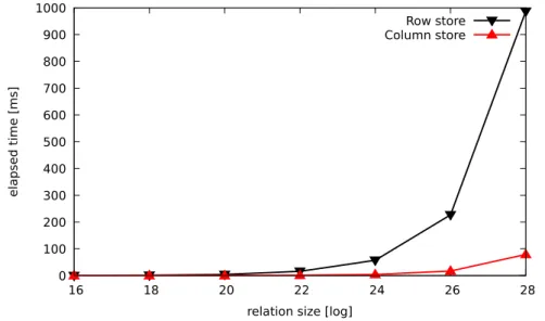
The scan operator is a fundamental operator in a database system as all other operators are built on top of the scan operator. Scan operations over columns in column stores are extremely efficient operations due to the locality of data items in the respective columns. A column scan operation exhibits a sequential access pattern, enabling the CPU prefetcher to bring into CPU cache the column items in advance, and this way minimizing the memory access latency. To show this, we have performed a small experiment showing the time it takes a sequential scan over a single attribute in a row store vs. column store.
2.3. Storage Layouts for a Main Memory Database System 0 100 200 300 400 500 600 700 800 900 1000 16 18 20 22 24 26 28 elapsed time [ms]
relation size [log]
Row store Column store
Figure 2.6.: Scan time in a row store and a column store over a single attribute
data were materialized in main memory in an instance of the movie structure shown in the code snippet in Section 2.3.1 and for the column store, in an instance of the structure shown in the code snippet above.
A number of relations were generated with cardinalities starting from 216and up to 228. The attribute values for the relation Movieswere picked randomly from a pool of movie data collected from IMDb. The query used in this experi-ment projects the values of the attributeyear: πyear(M ovies). The query was hand-coded in C++, and executed over both, the row and column store. The runtime of the scan operations for both, the row store and the column store were measured over all the relation sizes 216−228. The experiment was run in a machine with Intel Xeon E5-2690 v2 3.00GHz processor and 256 GB of main memory. The results of this experiment are shown in Figure 2.6.
As it can be seen in Figure 2.6, the scan operation in the column store is by far more efficient than the same operation over the row store. For example, if we look at the relation cardinality of 228, the scan operation in the column store is a factor of 12 cheaper than the same operation in the row store. Such a large difference in the runtime comes mainly from the fact that only the values of the attribute year were required in the query. In the column store, the scan operator iterates over the items of a single vector; the column items of the attribute year are narrow in width (i.e., 32 bits), therefore they fit nicely
into the CPU cache lines. In contrast to the column store, in the row store the tuples are much wider—they contain the values of all the attributes in the scanned relation—thus causing expensive cache misses. In column stores, the cache lines are filled with consecutive data items from the particular column being scanned, allowing for an optimal utilization of the cache. That is, the cache lines are not polluted with irrelevant data belonging to other attributes which are not required in a query. In row stores, all the attribute values of a tuple have to be brought into the cache lines even if the values of only a single
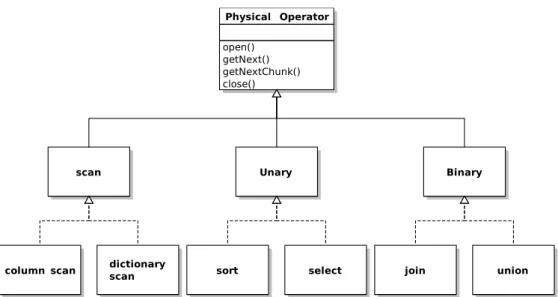
Figure 2.7.: An UML graph of physical operators in SystemTx
attribute are required, therefore, the cache lines are polluted with unnecessary data items. Of course, our experiment was biased towards column stores as the query projected the values from a single attribute only. Nevertheless, our experiment shows the superiority of column stores for applications that require reading large amount of data but from rather few columns, as it is the case with OLAP workloads.
2.4. Iterator Model
Query execution in traditional database systems consist of physical operators that implement an interface consisting of three primitive virtual functions:
open(), getNext(), and close(). This is known as the volcano-style [23] iterator-based query execution, or simply the pull model.
An UML class diagram of operators that implement these virtual functions in SystemTx has been depicted in Fig. 2.7. We separate the operators in three groups: scan operators, which basically scan the source of tuples, the second group consists of operators that consume tuples from a single input. The third and the final group consists of operators that consume tuples from two inputs, e.g., the left and the right input in a join operator.
A volcano-style query execution works by first having the root operator call the function open() on all its children operators all the way to the leaf opera-tors. In response to this call, each operator in the operator tree initializes its resources. A consumer operator, in this case the root operator pulls the tuples from its children operators by means of the function call getNext(). After the entire stream of tuples has been processed, the root operator propagates the function call close()to all its children operators, and as effect, all the operators receiving this call close their resources and release their buffers. This iterator model (pull model) is illustrated in Figure 2.8.
2.4. Iterator Model op1 op3 op5 scan[Ri] getNext() op4 scan[Ri] getNext() getNext() getNext() op2 scan[Ri] getNext() getNext()
Figure 2.8.: Illustration of the pull-based iterator model
from the pull data flow model, in that the stream of tuples are not pulled but rather pushed towards consumer operators by their children operators all the way to the root (top-most) operator. It has been shown in [52] that the push model allows for a better code and exhibits better data locality. We have, therefore, implemented the push model in our system.
In the literature, tuple producing operators are categorized into three groups: operators that produce tuple-at-a-time, operators that produce a block of tu-ples – chunkatatime, and the operators that materialize entire columns -column-at-a-time. In the following subsections, we briefly explain these groups of operators.
Tuple-at-a-time
Tuple-at-a-time is an iterator model used commonly in traditional database systems, whereby operators produce a single tuple for each getNext() function call. In this approach, operators do not materialize tuples, but they route them to their parent operator (consumer operators). This is known in database terminology aspipelining.
On the other hand, pipeline breakers are those operators that materialize their tuples before passing them to the next operator. A good example of a pipeline breaker is the hash-join operator. The tuples from one of its sides (recall that join operators are binary operators) are materialized in a hashmap structure, therefore the pipeline is broken. The tuples from the other side are then probed against the hashmap, and only if they qualify after this step, they flow to the next operator.
The main drawback with the tuple-at-the-time execution paradigm is that it incurs high interpretation overhead. Depending on the operator tree size and the selectivity of predicates, an arbitrary large number of function calls take place before a tuple is produced and has reached the root operator. That is, the functiongetNext()can be called million times or more to process a column, depending on the column size. In addition, each function invocation (e.g.,
getNext()) corresponds to a look-up in the virtual function table, thus adding more costs. As the function callgetNext()is routed from one operator to another,
the CPU cache has to be flushed and reloaded with operator specific instructions as well as operator data. Inadvertently, this leads to high cache miss-ratio, and causes expensive memory stalls.
Ailamaki et. al [3] show that 90 % of memory stalls in database systems are caused by first level (L1) I-Cache and second level (L2) D-Cache misses. First level I-Cache size is relatively small (in range of 4 - 32 KB), hence instruction misses occur often in the tuple-at-a-time iterator model even for a small operator tree size.
Chunk-at-a-time
Chunk-at-a-time is an execution scheme where instead of pipelining a single tuple, operators fill a chunk with tuples and pass an iterator (which is merely a memory reference) to their parent operator. An iterator in this context is a pointer that points to the chunk’s start address. We refer to the chunk as buffer, which has astart position, a size attribute, and anend position.
Chunk-at-a-time scheme has the advantage that only a memory address is routed from one operator to another instead of expensive copies of chunks. However, operators in this approach have to break the pipeline, due to buffer materialization, thus costing additional memory. The advantage of the chunk-at-a-time approach however is that it allows for block-oriented processing of tuples, thus reducing significantly the number of getNext() function calls. The latter is replaced by thegetNextBlock()function call which significantly amortizes the costs of the function callgetNext(), asgetNextBlock()is called on chunk-basis and not on tuple-basis, as it is the case with getNext(). In chunk-at-a-time, the consumer operators iterate over tuples in a chunk in a tight loop, e.g.:
for(Iterator* it = chunk.begin(); it != chunk.end(); ++it) { // do smth with a tuple, e.g., print it
print(*it); }
The processing of tuples in a tight-loop opens doors to the efficientvectorized execution, as such tuple iteration is not interrupted by the function calls get-Next(), i.e., more valuable CPU time is spent on operating over values than on function call overhead [7, 64]. This scheme opens doors for other optimizations such as loop-pipelining, automatic SIMD code generation by the compiler, less data cache misses due to high data locality (cache lines are filled with data from one chunk, thus less memory traffic). A notable system implementing this execution scheme is VectorWise [66].
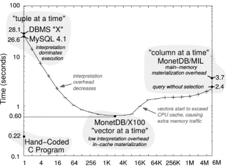
Chunks hold relatively small number of (cache resident) items and are ma-terialized incrementally. Chunks are implemented as an array (vector) in the actual code. The array size is a system parameter and it is set in accordance to the cache size, such that the arrays can fit into the CPUs L2 D-Cache. If arrays do not fit into the CPUs cache, expensive memory traffic between cache and main memory is caused. Such traffic forms a major bottleneck in main memory database systems. This is well illustrated in the Figure 2.9. According to the experiments in [65], as the vector size increases beyond 2K elements, they start
2.4. Iterator Model
Figure 2.9.: Illustration of tuple processing schemes. The x-axis denotes the vector size. Figure taken from [65].
spilling into main memory (they don’t fit any longer into the CPU cache), thus expensive memory traffic is caused.
Column-at-a-time
Systems like MonetDB [6] have taken the other extreme and materialize inter-mediate results - entire columns.
Materializing entire columns leads to the advantage that only one function call is required for processing all the tuples by a single operator. Just as in chunk-at-a-time execution model, this execution scheme opens ways for opti-mizations such as loop-unrolling, automatic SIMD instruction generation by compilers, etc. That is, tuple interpretation overhead is significantly reduced, however, at the price of high memory consumption. When working with large data sets, expensive memory traffic is caused by each operator, as operators will spend significant time writing into memory, and the intermediate results won’t fit into the CPU cache, see Fig. 2.9. This problem is further exacerbated with multi-CPUs which share their memory, as shown in [64].
3. SystemTx
In this chapter, we first present our main memory column oriented database system coined SystemTx. After a brief introduction of SystemTx, a section follows which presents the initial storage layout used in SystemTx. The initial storage layout was then replaced by a new storage layout as it caused high TLB miss rates when scanning multiple columns sequentially. The underpinnings of the new storage layout are the topic of the last section of this chapter.
3.1. Introduction
Although SystemTx is a main memory column store, we use rows/tuples as a representation of intermediate results. This allows for better cache locality during the evaluation of expressions. Second, we implemented thepush-based model, as it allows for better code and exhibits better data locality [52]. In a push-based model, each algebraic operator implements an interface withinit,
step, andclosefunctions. Thestepfunction is the most important. It accepts an input tuple, processes it, and passes it to the consumer operator up the tree via calling the step function of the consumer.
TX_Scan::run() {
for(i=0; i<|R|; ++i) {
t.rid=i; t.ap++; t.bp++; t.cp++ ... consumer.step(t);
} }
The RID variable and the column pointers in tupletare maintained by the scan operator (as depicted in the pseudo code above). This way, they point to the correct column values, and upon request, such column values can be fetched by means of the map operator, as shown in the code snippets below.
In SystemTx, there exist two ways of dereferencing (accessing) column values. The first method accesses column values based on row identifiers (RIDs). In pseudocode, this reads as:
Tx_MAP1::step(t) { t.A = R.A[t.rid]; t.B = R.B[t.rid]; t.C = R.C[t.rid]; ... consumer.step(t); }
The second method accesses column values based on column pointers Tx_MAP2::step(t) { t.A = *(t.ap); t.B = *(t.bp); t.C = *(t.cp); ... consumer.step(t); }
The column values are also stored in the tuple t, which is then passed to the next operator (consumer) in the operator tree.
The selection operator simply pipelines the qualifying tuples to its consumer operator.
Tx_Select::step(t) {
if(p(t)) consumer.step(t); }
3.1.1. Physical operators in SystemTx
In this section, we present physical operators implemented in the SystemTx that are of relevance to this thesis work.
Sequential scan operator scan(R) scans an input relation R by means of a tuple t. The tuple tcontains an attribute named RID, which represents the row identifier and pointers to columns of R; these pointers are offsets to the respective column values. The number of pointers in tupletis query dependent, that is, for each attribute required in a query, there is a pointer to the values of that attribute (i.e., column).
The scan operator iterates over all “tuples” by incrementing the pointers in t and the RID variable. The tuple t is pushed iteratively to the consumer operator via the consumer’s step method call as shown in the pseudo of the previous section.
Before we present the bypass selection operator, let us briefly recall the reg-ular selection operator defined in Section 2.1. The selection operator σp(e) :=
{t|t ∈ e∧p(e)} filters out all the tuples that do not satisfy the predicate p. The tuples that pass the predicate are passed up higher in the tree to the next operator.
Bypass selection operator σ+
p(e) := {t|t ∈ e∧p(e)} and σ−p(e) := e− σ+
p(e) ≡ {t|t∈e∧ ¬p(e)} in contrast to the regular selection operator bifur-cates the input stream into two disjoint streams; the true stream denoted by σ+
p(e), and the false stream denoted by σ−p(e), respectively. To this end, the two output streams are finally merged by the union operator ∪- (without an
expensive duplicate elimination, see Section 6.4), sitting on top of the plan. One should not think of the bypass selection operator as two operators, where one produces the true stream and the other one the false stream of tuples. This operator is implemented as a single operator σ± and produces both streams simultaneously. The benefits of the bypass selection operator are shown in
3.2. A Bad Storage Layout 0 5 10 15 20 25 30 12 14 16 18 20 22 24 26 28 time-per -tuple [ns]
relation size [log]
Intel(R) Xeon(R) CPU E5-2690 v2 3.00GHz 1 2 3 4 5 6 7 8 9
Figure 3.1.: Column access costs over the initial storage layout
Chapter 6. In the following, the pseudocode for bypass selection operator is shown. Tx_BYPSelect::step(t) { if(p(t)) { consumer_true.step(t); } else { consumer_false.step(t); } }
3.2. A Bad Storage Layout
In this section we present our initial storage layout used in our in-memory database system – SystemTx. In this storage layout relations are entirely kept in main memory, and they are vertically partitioned (DSM scheme), that is, attribute values of each attribute are stored in a separate column. Columns in turn are stored in separate vectors (i.e., arrays), just as in the example storage layout given in Section 2.3.2. A relation R may contain a number of such vectors depending on the number of attributes, whereby each vector represents an individual attribute ofR.
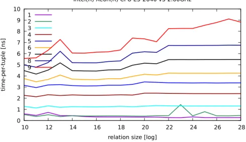
One important cost factor in a main memory column store is the cost of the dereferenciation operator used for column access [1]. The scan time of course is proportional to the cardinality of the column. Thus, several relation sizes must be tested. We were interested in the costs of scanning multiple (i.e., 1,2, . . . ,9) columns simultaneously. The measurements for such scans over our initial storage layout are contained in Figure 3.1. The x-axis is labeled by the base-2 logarithm of the relation’s cardinality. The y-axis presents the access
0 1 2 3 4 5 6 7 8 9 10 10 12 14 16 18 20 22 24 26 28 time-per -tuple [ns]
relation size [log]
Intel(R) Xeon(R) CPU E5-2640 v3 2.60GHz 1 2 3 4 5 6 7 8 9
Figure 3.2.: The effect of DTLB misses on a column store
time per column and row in nanoseconds. Each of the curves 1-9 corresponds to 1-9 simultaneous column scans.
From the cost function point of view, these curves are sub-optimal. They give the impression that they cannot be easily approximated with a high precision, i.e., an approximation yielding a small q-error (cf. Chapter 4). And indeed, the visual impression turned out to be true. Further, note the steep increase from relation size 221 to 222. To accurately model this steep ascent, additional relation sizes between these two points (221−222) would have to be generated and scan costs on these would have to be measured. Clearly, this would have a profound negative impact on the calibration time of the cost model. Last but not least, we were not satisfied with the high latency in column accesses, which as shown in Figure 3.1 are in order of 30 ns for 9 columns. To this end, our initial storage layout proved to be a bad basis for a query execution engine.
An analysis of the cause of this bad behavior revealed the following. The reason for the steep increase in the latency times is the high rate of L1 DTLB misses (details are given in Sec. 2.2.5). To understand why this effect only shows for more than 4 simultaneously scanned columns, it is important to know that the processor used is an Intel Xeon E5-2690 v2 3.00GHz processor. This processor has four prefetchers, explaining that there is virtually no difference in time between scanning 1 column and scanning 4 columns simultaneously. The second important piece of information is that the processor has a 4-way associative L1 DTLB. This explains why the curves go higher and higher for more than 4 simultaneous column scans. That is, the fixed stride in such column accesses operations lead to the eviction of DTLB entries. The last point is that the steep increase occurs only for relations with cardinalities larger than 221. This is explained by the small L1 DTLB size.
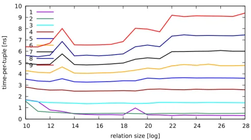
We have repeated the same experiment using newer hardware (Haswell and Skylake XEON processors). The results of this experiment are shown in
Fig-3.3. Storage Layout in SystemTx 0 1 2 3 4 5 6 7 8 9 10 10 12 14 16 18 20 22 24 26 28 time-per -tuple [ns]
relation size [log]
Intel(R) Xeon(R) CPU E5-2620 v4 2.10GHz 1 2 3 4 5 6 7 8 9
Figure 3.3.: The effect of DTLB misses on a column store
ures 3.2-3.3. In the new experiment with the new hardware, we see that the effects of the DTLB misses are not as severe as in the previous experiment. Nevertheless, in the next subsection we present a new storage layout which al-leviates the negative effect of DTLB misses regardless of the hardware (new or old), and in addition, the scan operations become cheaper.
3.3. Storage Layout in SystemTx
Having found the reason for the steep ascend in access time, we were looking for the cause within the initial storage layout. In the initial storage layout, during bulk load and during restart, system allocates huge chunks of memory, holding, whenever possible, a whole column of a given relation. This results in scan strides which suffer badly from L1 DTLB misses. Thus, we decided to implement a new storage layout. In the new storage layout, we changed (among other things we did not like either) the memory allocation strategy. Instead of allocating huge chunks for each column, we allocate multiple smaller chunks of memory for each column. These chunks are not of fixed size but instead are able to contain a fixed number of attribute values. Further, the allocation strategy goes round robin on the columns. This is illustrated in Figure 3.4. The green rounded rectangles represent the logical columns, and the white rectangles represent the column chunks, which in the figure are accidentally all of the same size. The line with the arrows demonstrates the timeline of the chunk allocation process. Each column maintains offset pointers (in an array) to the beginning of each of its constituent chunks. Using these pointers we can iterate over items belonging to a column as if they were stored contiguously in the memory. Since the chunk’s cardinality is known (is a global parameter), we do not risk overflowing the chunks when scanning columns. Upon scanning all the items belonging to a single chunk, we jump to the next chunk (belonging to
Figure 3.4.: Illustration of the chunk-wise storage layout in SystemTx the column that we are currently iterating) by following the next chunk pointer. Technical details on the allocator are presented in Appendix A.1.
The benefits of the new storage layout for the old and new hardware can be seen in Figures 3.5–3.7. The curves are now more streamlined, therefore allowing for better approximation by cost functions (cf. Chapter 4), and further, the absolute column scan costs have also dropped as a side-effect, which we warmly welcomed.
3.3. Storage Layout in SystemTx 0 0.5 1 1.5 2 2.5 3 3.5 4 4.5 5 12 14 16 18 20 22 24 26 28 time-per -tuple [ns]
relation size [log]
Intel(R) Xeon(R) CPU E5-2690 v2 3.00GHz 1 2 3 4 5 6 7 8 9
Figure 3.5.: Reduced DTLB miss effect using the new storage layout
0 1 2 3 4 5 6 12 14 16 18 20 22 24 26 28 time-per -tuple [ns]
relation size [log]
Intel(R) Xeon(R) CPU E5-2640 v3 2.60GHz 1 2 3 4 5 6 7 8 9
0 1 2 3 4 5 6 7 12 14 16 18 20 22 24 26 28 time-per -tuple [ns]
relation size [log]
Intel(R) Xeon(R) CPU E5-2620 v4 2.10GHz 1 2 3 4 5 6 7 8 9
4. Cost Estimation and Approximation
In this chapter, we present the cost model derived from our column store – SystemTx. Cost model presented in this chapter is used by the optimization algorithms presented later in Chapter 5 to Chapter 7.
The contents of this chapter were published in [33].
4.1. Introduction
The goal of the query optimizer is to find the optimal (i.e., the cheapest) plan from the space of all possible plans. Query optimizers discriminate the enu-merated plans based on their costs. Since the cost metric plays a decisive role in finding the “cheapest” plan, it is important that our cost model closely re-sembles the true costs of a plan, i.e., the cost of an actual execution of the plan. The cheapest plan doesn’t necessarily have to be the plan with lowest running time, it could be the one that minimizes the energy consumption (e.g., for databases running on handheld devices), or the time until the first tuple is produced. Nevertheless, in this chapter we assume that the cheapest plan is the one with the lowest total execution time.
In the new era of emerging main memory databases, the role of I/O costs has diminished, whereas the CPU costs have taken the dominating role. In main memory databases, CPU architectural characteristics such as the branch misprediction penalty can outweigh by far the costs of simple comparisons, therefore they should be well estimated by a cost model. Further, costs such as accessing column values, incrementing iterators, tuple pipelining etc., play an equally important role in a main memory database system.
In this chapter, we tackle two subproblems related to the cost model. First, we establish the cost functions, and second, we show how to obtain the param-eters for the cost functions.
Cost functions cannot model 100% error-free the true costs of a plan due to the speculative nature of modern CPUs, hierarchical memory etc. However, we should strive to minimize the error if the goal is to find the best plan, i.e., the plan with the lowest execution costs. The majority of the cost function in the literature minimize the`2 error. Since`2 does not provide bounds on error, it is not suited for query optimization. In this thesis, we approximate the cost functions under the q-error. Approximation under the q-error, it turn, provides us bounds on the quality of the approximation. In the light of q-error, we present two important findings: (1) we show that if our cost function is precise up to a factor q, then the plan picked by our optimizer under this (erroneous) cost function is atmost a factor of q2 far from the optimal plan. That is, we show a direct link between the error of the cost functions and the plan quality.
Although a direct link between the error of the cardinality estimation and the plan quality has been shown in [48], we show for the first time that there is also a direct link between the error of the cost function and the plan quality. (2) We show that if the q-error is bounded by a small q, then the best plan picked by the optimizer is still the optimal plan.
Cost functions depend on cardinalities. In Chapter 8, we present an efficient method based on sampling which can be used to find the selectivities for all the subsets of predicates given in a query.
The rest of the chapter is organized as follows. Related work is described in Section 4.2. In Section 4.3 we define the q-error, whereas in Section 4.4 we show its theoretical implications for our cost model. In Section 4.5 we state the cost functions for the physical operators scan, selection (σ), and the map (χ) operator. Additionally, we provide cost functions for th