Mixture Modeling and Outlier Detection in Microarray Data Analysis

(1)

A Dissertation by

NYSIA I. GEORGE

Submitted to the Office of Graduate Studies of Texas A&M University

in partial fulfillment of the requirements for the degree of DOCTOR OF PHILOSOPHY

August 2008

(2)

A Dissertation by

NYSIA I. GEORGE

Submitted to the Office of Graduate Studies of Texas A&M University

in partial fulfillment of the requirements for the degree of DOCTOR OF PHILOSOPHY

Approved by:

Chair of Committee, Naisyin Wang Committee Members, Raymond J. Carroll

Robert Chapkin Erning Li

F. Michael Speed Head of Department, Simon J. Sheather

August 2008

(3)

ABSTRACT

Mixture Modeling and Outlier Detection in Microarray Data Analysis. (August 2008)

Nysia I. George, B.S., Texas A&M University; M.S., Texas A&M University

Chair of Advisory Committee: Dr. Naisyin Wang

Microarray technology has become a dynamic tool in gene expression analysis because it allows for the simultaneous measurement of thousands of gene expressions. Uniqueness in experimental units and microarray data platforms, coupled with how gene expressions are obtained, make the field open for interesting research questions. In this dissertation, we present our investigations of two independent studies related to microarray data analysis.

First, we study a recent platform in biology and bioinformatics that compares the quality of genetic information from exfoliated colonocytes in fecal matter with genetic material from mucosa cells within the colon. Using the intraclass correlation coefficient (ICC) as a measure of reproducibility, we assess the reliability of density estimation obtained from preliminary analysis of fecal and mucosa data sets. Nu-merical findings clearly show that the distribution is comprised of two components. For measurements between 0 and 1, it is natural to assume that the data points are from a beta-mixture distribution. We explore whether ICC values should be modeled with a beta mixture or transformed first and fit with a normal mixture. We find that the use of mixture of normals in the inverse-probit transformed scale is less sensitive

(4)

toward model mis-specification; otherwise a biased conclusion could be reached. By using the normal mixture approach to compare the ICC distributions of fecal and mucosa samples, we observe the quality of reproducible genes in fecal array data to be comparable with that in mucosa arrays.

For microarray data, within-gene variance estimation is often challenging due to the high frequency of low replication studies. Several methodologies have been developed to strengthen variance terms by borrowing information across genes. How-ever, even with such accommodations, variance may be inflated by the presence of outliers. For our second study, we propose a robust modification of optimal shrink-age variance estimation to improve outlier detection. In order to increase power, we suggest grouping standardized data so that information shared across genes is similar in distribution. Simulation studies and analysis of real colon cancer microarray data reveal that our methodology provides a technique which is insensitive to outliers, free of distributional assumptions, effective for small sample size, and data adaptive.

(5)

(6)

ACKNOWLEDGEMENTS

I have tremendous and unreserved appreciation for my advisor, Dr. Naisyin Wang. Finite words cannot express how blessed I am by her mentorship in my life. Dr. Wang is a very special person and many times went above and beyond the call of duty. She saw qualities in me that I never saw in myself and fully committed herself to investing in me as a future colleague. Through her guidance, I have gained confidence to explore and develop my statistical ideas and intuition. I learned a lot through our talks, which always complimented her insight, expertise, and passion for professional growth.

I also salute Drs. Michael Speed and Raymond Carroll for the special role each played during my graduate studies. I thank both of them for being a resource and reaching out to me in ways that stretched far beyond academia. Along with Dr. Speed and Dr. Carroll, I would like to thank the other members of my committee -Dr. Robert Chapkin and -Dr. Erning Li. I could not have asked for a more supportive committee.

Praise God for my family who is probably most excited to celebrate with me - I am no longer a professional student! My family has shown me unconditional love and has forever supported my education and career aspirations. I am thankful to have them rooting me on. Undeniably, my mom is the best cheerleader anyone could hope for.

Additionally, I extend a heartfelt thanks to my spiritual family. I could not imagine completing this journey without them. The endless prayer, words of en-couragement, and sound advice were my anchor. They were always available when I needed support and most importantly, continuously reminded of the love, grace, and

(7)

power of God. I offer special thanks to Danielle and Ra’sheedah, my roommates and spiritual sisters, for their love, friendship, and comic relief.

Finally, I thank God for imparting in me all that He is. He truly opened my eyes to new heights that I can reach through Him. Through this process, He taught me about endurance and standing firmly on the promises He has spoken to me. I am honored that He entrusted me with such an amazing accomplishment.

(8)

IV VARIANCE ESTIMATION AND OUTLIER DETECTION METHODOLOGY . . . . 27

(9)

4.3 Variance Estimation Methodologies . . . 30

4.4 An Overview of Outlier Detection . . . 38

4.5 Outlier Detection Methodology . . . 40

V ANALYSIS OF OUTLIER DETECTION FOR SIMULATED MICROARRAY DATA . . . . 43

5.2 Simulation I: Independent Gene Variance-Intensity Re-lationship . . . 43

5.3 Simulation II: Gene Variance-Intensity Dependency . . . . 49

VI ANALYSIS OF OUTLIER DETECTION FOR REAL DATA . . 55

6.2 Data Description . . . 56

6.3 Data Normalization . . . 57

6.4 Colon Cancer Microarray Data Analysis . . . 60

VII CONCLUSION . . . . 72

REFERENCES . . . . 76

APPENDIX A ADDITIONAL ANALYSIS OF SIMULATED STUDIES PRESENTED IN CHAPTER V . . . . 83

APPENDIX B ADDITIONAL ANALYSIS OF REAL DATA PRESENTED IN CHAPTER VI . . . . 86

(10)

LIST OF TABLES

TABLE Page

1 Monte Carlo mean, bias, standard deviation, and square-root MSE (RMSE) of estimates from simulation study ”Data Generated from

Beta-mixtures, Fit with Normal-mixtures.” . . . 23 2 Monte Carlo mean, bias, standard deviation, and square-root MSE

(RMSE) of estimates from simulation study ”Data Generated from

Normal-mixtures, Fit with Beta-mixtures.” . . . 24 3 P(X2 _{> χ}2

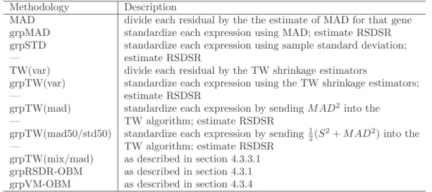
0.05,k−1) for fecal (mucosa) data using 5, 8, and 12 bins. . . 25 4 Descriptive procedures for ten methodologies of estimating

gene-specific variance. . . 45 5 The average number of detected outliers for simulated data with

no outliers. . . 46 6 Positive Predictive Value (PPV) and False Negative Rate (FNR)

of outlier detection methodologies for simulated data perturbed

by outliers. . . 47 7 Positive Predictive Value (PPV) and False Negative Rate (FNR)

of outlier detection methodologies for simulated data with

mean-variance relationship perturbed by outliers. . . 53 8 The number of outliers detected at Q=0.01 in real data when using

grpRSDR-OBM, grpTW(mix/mad)-OBM, and grpVM-OBM to

estimate within-gene variance. . . 61 9 Average BEED-MAD ratio for detected outliers when using

grpRSDR-OBM and grpTW(mix/mad)-grpRSDR-OBM to estimate gene variability. . . . 63 10 Number of detected outliers (average BEED-MAD ratio) for

de-tected outliers when using grpRSDR-OBM and

(11)

11 Positive Predictive Value (PPV) and False Negative Rate (FNR) of outlier detection methodologies for simulated data perturbed

by outliers added to every 10th _{gene. . . .} ₈₃

12 Positive Predictive Value (PPV) and False Negative Rate (FNR) of outlier detection methodologies for simulated data perturbed

by outliers added to every 20th _{gene. . . .} ₈₄

13 Positive Predictive Value (PPV) and False Negative Rate (FNR) of outlier detection methodologies for simulated data with mean-variance relationship perturbed by outliers added to every 10th

gene. . . 85 14 Positive Predictive Value (PPV) and False Negative Rate (FNR)

of outlier detection methodologies for simulated data with mean-variance relationship perturbed by outliers added to every 20th

gene. . . 85 15 Number of detected outliers (average BEED-MAD ratio) for

de-tected outliers when using grpTW(mad50/std50)-OBM to esti-mate gene variability for genes with complete data and those with

(12)

LIST OF FIGURES

FIGURE Page

1 Histogram of ICC values. . . 19 2 Histogram of IPT-ICC values. . . 20 3 Plot of the IPT-ICC values, fitted mixture of normal distribution,

and pdf of transformed beta random variables for the (a) fecal and

(b) mucosa data. . . 21 4 Density plots of the difference between estimated variances and

the true variance for simulated N(0,1) gene expression data. . . 36 5 The number of false negatives classified by two methods using one

gene expression data set simulated to have no relationship between

gene center and spread. . . 50 6 The number of false positives classified by two methods using one

gene expression data set simulated to have no relationship between

gene center and spread. . . 50 7 A report of false negatives and false positives for gene expression

data simulated to have no relationship between gene center and spread. 51 8 Two methods of reducing systematic bias in gene expression data.

Data are taken from treatment Acp. . . 59 9 Scatterplot of residual values for genes with outlier expressions for

Acp data. . . 65 10 Scatterplot of residual values for genes with outlier expressions for

(13)

CHAPTER I

INTRODUCTION

Microarray technologies simultaneously measure the expression levels of thousands of genes and are widely used in biomedical research. Because these high-throughput instruments facilitate large-scale experiments and advanced research, microarray data analysis is constantly progressing. New statistical methodologies for analyzing gene expression data are emerging in order to gain biological insights. This dissertation presents two independent studies of microarray data analysis. The methods that we develop for both topics are very applicable and their considerations are necessary to accurately analyze microarray data sets.

Our first work is motivated by the need to evaluate fecal mRNA microarray reproducibility. We study a recent platform in biology and bioinformatics that com-pares the quality of genetic information from exfoliated colonocytes in fecal matter with genetic material from mucosa cells within the colon. Colon cancer is a leading cause of cancer death and it believed that attitudes towards the colonoscopy are a deterrent for colorectal cancer screening. The goal is to offer patients an alternative so that those who are at-risk for cancer are diagnosed and treated at an early stage. To address the issue of gene reproducibility between the two platforms, we use the intraclass correlation coefficient (ICC) as a measure of reproducibility. For measure-ments between 0 and 1, it is natural to assume that the data points are from a beta distribution. As an alternative, consider the fact that a uniform random variable after

(14)

being transformed by the inverse-probit function will be normally distributed, where the probit function is the cumulative distribution function (CDF) of the standard normal distribution. This suggests that a plausible distributional assumption for the inverse-probit transformed ICC values is the normal distribution. Both are consid-ered to be acceptable approaches. However, will both lead to comparable results? If not, then under what circumstances does one model fail? These are the questions we wish to address.

Chapters II and III of this dissertation are devoted to our first study. In Chap-ter II we give a complete description of the problem and discuss the details of each methodology used in the data analysis. In Chapter III we explore whether ICC values should be modeled with a beta mixture or transformed first and fit with a normal mixture. We carry out a simulation study and use the chi-square goodness of fit test to determine the accuracy of each model. We are particularly interested in the effect of transformation under model mis-specification.

Secondly, we introduce statistical tools to improve variance estimation and out-lier identification in microarray data. A core goal of microarray analysis is to identify an informative subset of differentially expressed genes under different experimental conditions. Typically, this is done through hypothesis testing, which relies on test statistics that properly summarize and evaluate information in the sample(s). A reliable variance estimator that is applicable to all genes is important for analysis. In microarray analysis we often find that genome-scale expression analysis generates large data sets with a small number of replicates for each gene. The widespread statistical limitations due to low replication make it necessary to devise adaptive methods for estimating gene-specific variance. Further complicating variance esti-mation is the frequent presence of outliers in microarray data. Not only is outlier identification critical for reliable estimation of variance, but we also require accurate

(15)

variance estimation in order to successfully identify outliers.

In Chapter IV, we introduce several variance estimation methodologies and out-lier identification procedures. We propose a robust modification of optimal shrinkage variance estimation (Tong and Wang, 2007). Our variance estimator is uninfluenced by outliers and allows for gene-specific, rather than pooled, estimates of variance. Additionally, we stabilize estimators by allowing each variance estimate to be the product of a gene-specific and common variance estimate. In order to increase power, we estimate the common variance term by grouping standardized data so that in-formation shared by genes post-standardization can be more efficiently utilized. For outlier detection we adopt a technique which is based on the false discovery rate approach.

Chapter V describes the setup of two simulation studies. The first setup does not assume any relationship between gene variability and location center, while the second is structured such that variance is modeled as a quadratic function of mean. These studies are used to compare the performances of numerous variance estimators and adaptive methodology.

In Chapter VI, we investigate the performance of variance estimation and outlier identification on colon cancer microarray data. We introduce the between extreme expression deviation to MAD (BEED-MAD) ratio statistic as an assessment tool for outlier classification when the truth is unknown.

(16)

CHAPTER II

MIXTURE MODELING OF THE INTRACLASS CORRELATION COEFFICIENT

2.1 Introduction

Microarrays, which measure gene expressions at the transcription level where RNA is made from DNA, take us from the days of detecting messenger RNA (mRNA) expression of a single gene to the current stage in which scientists can simultaneously measure the expression of thousands of genes. Daily improvement in this technology frequents the production of new assays and new microarray data platforms. Among them, and of particular interest, is a recent development that enables the collection of genomic information from exfoliated colonocytes in fecal matter. It is known that an early detection of cancerous colon cells results in high cure and survival rates among colon cancer patients. However, people tend to shy away from invasive procedures such as the colonoscopy. Consequently, it is of great interest to develop non-invasive early detection instruments.

Although evidences exist in the fecal platform that partially degraded mRNA in fecal samples can produce meaningful measurements (Schoor et al., 2003), and the conclusions by Davidson et al. (2003) and Kanaoka et al. (2004) suggest that it is possible to isolate intact fecal eukaryotic mRNA, it is unknown whether one can expect the same quality from the large amount of fecal microarray data. The current study, to the best of our knowledge, is the first one that investigates and reports the reproducibility of fecal microarray data.

Biological variation in gene expression data can be assessed with subject to sub-ject replication. In order to determine if one can successfully obtain the same findings

(17)

from the same biological sample when the experiment is repeated, it is necessary to determine whether the gene expression levels of a gene from the same subject behave more similarly to each other compared to those of the same gene from different sub-jects. One can observe this type of similarity even when the biological samples from the same subject are processed through two independent bioassays, as is done for samples using different biological materials. Precisely, under the best scenario that the same biological sample is used, we evaluate the similarity between independent results produced by the same bioassay in a lab. While we focus only on subject to subject variation, we acknowledge that there are other types of replication in gene expression data (Nguyen et al., 2002).

In order to assess the agreement between measurements from microarray data collected from the same subject we use the intraclass correlation coefficient as a reliability index (Carrasco and Jover, 2002). Intraclass correlation (ICC), defined in simplest terms as a measure of reproducibility, is used as a statistical measure to assess methodological and biological variation in DNA microarray analysis. The larger the intraclass correlation coefficient, the more differentiation among gene readings collected from different biological samples relative to that among readings using the same biological material. Thus, an ICC value near 1 signifies a strong indication of reproducibility and agreement between experiments. On the other hand, if the ICC is near 0, then within-subject variance is relatively large compared to between-subject variance and it is likely that one can not obtain the same expression level in a repeated experiment.

Considering how replicative arrays are produced, it may be harder to recognize the phenomenon commonly associated with ”reproducibility” when a gene is neither up nor down regulated. Although the same biological materials are produced, the dominating variation could be caused by the two different bioassay processes. If this

(18)

is true, then we expect to observe at least a small proportion of genes to always have low reproducibility, thus resulting in a mixture model for the distribution of ICC val-ues. The use of mixture-modeling in bioinformatic research is not new. Researchers have devoted much attention to methodology that can appropriately separate gene expressions into meaningful groups. Allison et al. (2002) and Ji et al. (2005) use beta-mixture modeling to describe distributional properties of different genes’ corre-lation coefficients. Like measurements of ICC, the values of correcorre-lation coefficients are between 0 and 1. On the other hand, He et al. (2006) and McLachlan et al. (2006) prefer the use of normal mixture distributions which eliminate the (0,1)-range constraint.

In a study comparing the fecal and mucosa bioarray platform we obtained con-flicting results when modeling inverse-probit transformed ICC (IPT-ICC) values with a component normal distribution and when modeling ICC values with a two-component beta distribution. It is our conjecture that, considering the boundary problem of the beta distribution, normal mixture modeling might be less sensitive to-ward model mis-specification. We have observed components of the beta mixture to be strictly decreasing with the density f(y|α, β) approaching infinity. This phenomenon causes the maximum likelihood estimate (MLE) of β parameters to be unstable. In order to address which of the two mixture models more accurately analyzes ICC val-ues of gene expression levels, we conduct a simulation study. Our ultimate goal is to select the better of the two systems to ascertain whether the fecal array samples share similar reproducibility as the mucosa array samples.

2.2 Methods

In order to carry out this analysis, we rely on numerous statistical methods. These methodologies are described in detail in the following subsections.

(19)

2.2.1 The Intraclass Correlation Coefficient

As with most measurements, measuring gene expression levels even from the same biological materials involves measurement error. In order to assess the agreement between measurements, we look to intraclass correlation coefficients whose use in genomic study was promoted by Carrasco and Jover (Carrasco and Jover, 2003). In-traclass correlation, in its simplest term, is defined as a measure of reproducibility. Consider the following simple model where the response Yij =ai+eij is thejth

mea-surement collected from theith subject. Further, variablesai andeij are independent

with means 0 and variance σ2

a and σe2, respectively. ICC is the ratio of the variance

between subjects to the total variance and is given by the following equation: ICC = σa2

σ2

a+σe2

, (2.1)

where σ2

a represents the between-subject variation, σe2 is the within-subject variance,

and 0 ≤ ICC ≤ 1. In the situation that samples from the same subject give an identical reading, then σ2

e = 0 and ICC = 1. We have perfect reproducibility. On

the other hand, if all the ai are close to zero such that the different measurements

corresponding to the same subject give the dominating variation, then we expect the ICC to be small.

Here, we use the ICC as a statistical measure to assess methodological and bi-ological variation in DNA microarray analysis. The larger the intraclass correlation coefficient, the more differentiation among gene readings collected from different bi-ological samples relative to that among readings using the same bibi-ological material. Thus, an ICC value near 1 signifies a strong indication of reproducibility and agree-ment between experiagree-ments. On the other hand, if the ICC is near 0, then within-subject variance is relatively large compared to between-within-subject variance and it is likely that the actual gene expression is irreproducible.

(20)

Shrout and Fleiss (1979) give guidelines for choosing among six different forms of the ICC, where each form is specifically defined by the experimental design and intent of the study. Since our design has each subject under different treatments measured by 1-2 randomly selected microarrays, we let the measurements from the same subject share the same random intercept and let the different treatments be the fixed effect. We then use this mixed-effects model to obtain the overall and random intercept variation and set them to be the denominator and numerator of the ICC value.

Classifying the ICC as a measure of reproducibility has long been in debate. Lin (1989) discusses two drawbacks that discredits the ICC as a reliable reproducibility index. First, it allows duplicate readings to be interchangeable in the sense that dupli-cate readings are considered as replidupli-cates rather than two distinct readings. Secondly, it is faulted for assessing uncorrelated paired readings with negative values. However, Carrasco and Jover (2003) argue that the ICC is a valid measure of agreement among microarrays and identify it as one of the most popular aggregate procedures used in measuring the agreement of continuous-scaled data. An aggregate procedure is characterized by its use of a single measure to assess agreement, whereas a disaggre-gate approach calculates agreement for each component of the measurement model separately (Carrasco and Jover, 2003).

2.2.1.1 Obtaining ICC Values for Genes on a Microarray Chip

We define a data observation Y_ijk[g] as being the gene expression g for subject i, treat-ment j, and array k. The observations are modeled by

Y_ijk[g] =µ[_jg]+a[_ig]+e[_ijkg], (2.2) for

(21)

i= 1,2, . . . , I, j = 1,2, . . . , J, and k = 1,2, . . . , Kij

This describes a microarray experiment where we consider I subjects, J treatments, and Kij arrays for subject i under treatment j. Also, µj is the overall mean for the

jth _treatment, _a

i ∼ N(0, σ2a) is the random effect due to the different subjects, and

eijk ∼ N(0, σe2) is the random effect due to array to array replication. We assume

that the error terms, eijk, are iid.

After having formulated the model for the data observations taken from the microarray, we can easily characterize the ICC for each gene. The following expression for ICC allows us to quantify the reproducibility index of gene g.

ICCg = σ2 a,g σ2 a,g+σe,g2 , g = 1,2, . . . , G, (2.3) where G is the number of genes.

2.2.2 Two-Component Mixture Models

The numerical findings of ICC and IPT-ICC values clearly show that the data comes from a mixture of two populations. Thus, we analyze the data as clusters to minimize within-group variance and maximize between-group variance.

When data is modeled by a mixture of two distributions we suppose that an observation comes from distribution 1 with probability π or from distribution 2 with probability 1−π. SupposeZi is a random indicator variable such that

Zi =      1, with prob =π 0, with prob = 1−π

Let Wi be the actual outcome observed through the process. Then Wi is distributed

as follows: Wi ∼      f1(w), Zi = 1 f2(w), Zi = 0,

(22)

where f1 and f2 are the probability density functions of distributions 1 and 2, respec-tively. If we consider the joint distribution of (W,Z), then

f(w, z) = f(w|z)f(z). Thus,

f(w) =P_zf(w|z)f(z)

and the resulting probability distribution function is given by

f(w) = πf1(w) + (1−π)f2(w) (2.4)

Furthermore, if we observe W =W1, . . . , Wn, the likelihood function is n

Y

i=1

[πf1(wi) + (1−π)f2(wi)]. (2.5)

2.2.3 Parameter Estimation using Expectation-Maximization Algorithm

We use the expectation-maximization (EM) algorithm (Dempster et al., 1977) to obtain parameter estimates of the mixture distributions. The EM algorithm is an iterative approach for estimation of incomplete data problems. Given starting values of the model parameters, the EM algorithm iteratively updates the estimates until a specified convergence is reached. In Sections 2.2.3.1 and 2.2.3.2 we describe pro-cedures for estimating the two-component mixture of beta and normal distributions, respectively.

2.2.3.1 Mixture of Beta Distributions

Suppose y1, . . . yn are n independent observations from fY(y|θB), where fY is the

density of a beta distribution and θB = (π, α1, α2, β1, β2). Let the random vector X = (Z, Y) = {zi, yi}, wherezi is an indicator variable which assumes the value 1 (0)

(23)

In the algorithm, we iteratively perform the “E” and “M” steps with the ’com-plete’ data likelihood function, L(θB|yi), for θB being

L(θB|yi) = n

Y

i=1

πf(yi|α1, β1) + (1−π)f(yi|α2, β2) (2.6) and the corresponding log-likelihood being

`(θB|yi) = n X i=1 log[πf(yi|α1, β1) + (1−π)f(yi|α2, β2)]. (2.7) In the E-step, z is updated with its conditional expectation given the observed data y. Consequently, z_i(k) = E[zi|yi,πˆ(k),αˆ1(k),αˆ (k) 2 ,βˆ (k) 1 ,βˆ (k) 2 ] = ˆπ(k)f(yi|α (k) 1 , β (k) 1 ) ˆ π(k)_f(y i|α(1k), β1(k)) + (1−πˆ(k))f(yi|α(2k), β2(k)) , (2.8) where the super index, k, denotes an estimate at the kth _iteration.

In the M-step of the EM algorithm we usez_i(k)to estimate the mixing proportion, where ˆ π(k+1) ₌ P_n i=1z (k) i n , (2.9)

and obtain maximum likelihood estimates of ˆα1, ˆα2, ˆβ1, and ˆβ2 numerically. The E-and M-steps are iterated until the convergence criteria is met.

The starting values forα1,α2,β1, andβ2 were set to 0.01 and{zi}was initialized

by setting one half of the indicator variables equal to 0 and the other half equal to 1 so that ˆπ(0)_{=0.50. We utilize the ’optim’ function in R to obtain parameter estimates} for the two beta density functions. The procedure was repeated until we observed a negligible change in the value of the log-likelihood given in (2.7).

(24)

2.2.3.2 Mixture of Normal Distributions

Let x1, . . . , xn be n iid observations from fX(x|θN), where fX is the density of a

normal distribution and θN = (π, µ1, µ2, σ12, σ22). In order to estimate the parameters for a two-component normal mixture, we use the MCLUST software package for R (Fraley and Raftery, 1999). MCLUST implements the EM algorithm (Section 2.2.3.1) to carry out the computations of a maximum likelihood approach for normal mixture modeling. For model selection, Mclust determines the number of clusters and the clustering model by maximizing the Bayesian Information Criterion (BIC) (Schwartz, 1978).

See Fraley and Raftery (1999) and Fraley and Raftery (2002) for more details regarding the MCLUST software package.

2.2.4 Distribution of Transformed Random Variables

In our simulation study of mixture model mis-specification, it is necessary to define the distribution of transformed random variables. In Section 2.2.4.2, we describe the distribution of probit transformed normal random variables (Normal → Beta). Likewise, in Section 2.2.4.1 we describe the distribution of inverse-probit transformed beta random variables (Beta →Normal).

2.2.4.1 Normal → Beta

Let X be a random variable from a two-component normal mixture model with prob-ability density function (pdf) fN given by

fN(x) =π φ(x;µ1, σ21) + (1−π) φ(x;µ2, σ22), (2.10) where 0 < π < 1 and φ(x;µi, σi2) is the pdf of a normal random variable with mean

(25)

Furthermore, consider transforming the data via the probit transformation given by Y = Φ(X). Then the density function of Y is given by

fB(y) = fN(g−1(y)) ¯ ¯ ¯ ¯_dyd g−1(y) ¯ ¯ ¯ ¯ = fN(g−1(y)) ¯ ¯ ¯ ¯_g0_{_g−11_(y)_} ¯ ¯ ¯ ¯ = fN(Φ−1(y)) ¯ ¯ ¯ ¯_φ_{_Φ−11_(y)_} ¯ ¯ ¯ ¯. (2.11) 2.2.4.2 Beta → Normal

Let Y be a random observation from a two-component beta mixture model with pdf fB given by fB(y) =π f(y|α1, β1) + (1−π) f(y|α2, β2), (2.12) where 0 < π <1 and f(y|αi, βi) = yαi−1₍₁₋_y)βi−1 R₁ 0 tαi−1(1−t)βi−1dt f(y|αi, βi) = yαi−1₍₁₋_y)βi−1 B(αi, βi) (2.13) is the pdf of a beta random variable with shape parameters αi, βi, for i= 1,2

We consider transforming the observations using the inverse-probit transforma-tion by letting X = g(Y) and g(·) = Φ−1₍_·_{). Then the range of} _X _{becomes (}_−∞_,_∞₎ and its density function is expressed as

fN(x) = fB(g−1(x)) ¯ ¯ ¯ ¯_dxd g−1(x) ¯ ¯ ¯ ¯ = fB(Φ(x))|φ(x)|. (2.14)

2.2.5 Chi-square Goodness of Fit

Let X1, . . . , Xn be an observed dataset. Suppose we divide the range of the data

(26)

the expected number of observations for that bin, we are able to use the Pearson’s chi-square (χ2_{) goodness of fit test to assess how well the proposed distribution fits} the observed data. The χ2 _{statistic for testing the null hypothesis} _H

0 : The data follow the specified distribution, is

X2 ₌ k X i=1 (Oi −Ei)2 Ei , (2.15)

where Oi and Ei are the observed and expected, respectively, frequencies for bin i.

To ensure that the expected frequency count is never zero, data is binned according to the following quantiles of observed data: 0, k−1 equally spaced values between 0.025 and 0.975, and 1. This results in k disjoint bins.

If a dataset is fit with a mixture of normal distributions, then the density function defined in (2.10) is used to determine the expected frequencies. Likewise, we use (2.14) to calculate expected frequencies when a dataset is fit with a mixture of betas. The cdf of (2.14) does not have a closed form solution. Thus, for both distributions, the area of a given bin is approximated with the trapezoidal rule for computing a Riemann sum. The trapezoid approximation of R_abf(x)dxassociated with a partition a =x0 < x1 < . . . < xn=b is

T = 1

2[f(x0) + 2f(x1) +. . .+ 2f(xn−1) +f(xn)] ∆x. (2.16) Each of the k intervals is divided into 4 equal parts so that n = 4 and ∆x= b−a

4 . 2.2.6 Likelihood Ratio Test

We use the likelihood ratio test in order to test for distributional differences in the reproducibility of fecal and mucosa samples. Let L1 be the maximum value of the likelihood without placing any assumptions on the model parameters. L1 is evalu-ated by substituting the maximum likelihood estimates for the unknown unrestricted

(27)

parameters. Let L0 be the maximum value of the likelihood function when the pa-rameters are restricted by assumptions placed on the model. We can then define the likelihood ratio statistic by

λ= L1 L0 .

Furthermore, let us assume that k parameters were lost by moving from the unre-stricted to the reunre-stricted setting. Under the reunre-stricted model, asn→ ∞, 2 logλ→χ2

k

in distribution. The likelihood ratio test rejects the testing assumption if 2 log λ > χ2

(28)

CHAPTER III

DATA ANALYSIS AND SIMULATION STUDY OF ICC VALUES

3.1 Introduction

We begin this chapter with a description of the fecal and mucosa data used in the study. In Section 3.3 we present the nature of the problem by showing discrepancies in the beta mixture fit of ICC values and the normal mixture fit of IPT-ICC values. Section 3.4 discusses a simulation study that was carried out to analyze sensitivity to model mis-specification. Finally, in Section 3.5 we compare the ICC distributions of fecal and mucosa samples in order to evaluate the quality of reproducible genes between the two platforms.

3.2 Fecal and Mucosa Data Description

Gene expression levels from the colon mucosa and fecal data samples were collected using the CodeLink System. From the thousands of genes included in both data sets, our working data set of statistically significant genes consisted of 2171 genes for the fecal data and 2241 genes for the mucosa data. The bioassays that were used to extract fecal mRNA were developed much later than the mucosa data used in this study, which was collected earlier in a different experiment. Although we did not have access to the original dataset, the available summary statistics were sufficient for us to produce ICC measurements.

3.2.1 Fecal Data

The fecal array data were collected from rat fecal samples in a study designed to explore the affect that diet has on genes being differentially expressed after exposure

(29)

to carcinogen/radiation (Liu et al., 2005). Rats in the study were exposed to carcino-gen azoxymethane (AOM) and randomly assigned to one of four different treatments resulting from a 2×2 factorial design. The two experimental factors were diet - fish oil/pectin (D1) and corn oil/ cellulose (D2), and radiation - with radiation exposure (IRT) and without radiation exposure (RCT). Fecal samples were collected 14 weeks after the last exposure to carcinogen AOM. There are respectively 7, 6, 8, and 7 bioar-rays collected under IRT-D1, IRT-D2, RCT-D1, and RCT-D2, respectively. Genes which were not disqualified and which had at least 3 usable replicates were kept. 3.2.2 Mucosa Data

Spraque Dawley rats used in the study to obtain mucosa array data were randomly assigned in a 3×2×2 factorial experiment to a treatment with diet, exposure, and time points as factors (Davidson et al., 2004). Corn oil/n-6 polyunsaturated fatty acid (PUFA) or fish oil/n-3 PUFA or olive oil/n-9 monounsaturated fatty acid (MUFA) was used as the dietary fat source; carcinogen AOM was used as the exposure source; time points were either 12 hours or 10 weeks after the first injection. The units were terminated at the appropriate time point in order to remove the mucosal layer from each colon so that RNA could be extracted from the mucosal samples.

3.3 Preliminary Data Application

The original ICC values were fit with a two-component beta mixture using the EM algorithm, producing the following density estimation for the fecal and mucosa data, f_Bf and fm

B respectively,

f_Bf(.; ˆθB) = 0.50Beta(0.30,0.64) + 0.50 Beta(0.27,0.63)

fm

(30)

After transforming the original ICC values via the inverse-probit transformation, we estimate the following two-component normal mixture densities for the fecal and mucosa data, f_Nf and fm

N respectively,

f_Nf(.; ˆθN) = 0.72 N(0.04,0.84) + 0.28N(−3.50,0.07)

f_Nm(.; ˆθN) = 0.81 N(−0.29,0.64) + 0.19N(−3.35,0.12).

A simple observation of the difference in proportion estimates for fecal and mu-cosa data leads us to question the accuracy of the two fits. It is unclear what the proportion of reproducible genes (upper component of the two mixtures) for fecal samples should be, 0.50 or 0.72? Unfortunately, the answer to this question depends on the mixture model we use to fit the data.

It is well known that when α < 1 (β < 1), the beta distribution increases to infinity at the lower (upper) endpoint, respectively. We find this to be the case with components of the beta mixture for both data sets. This phenomenon is easily seen in the graphs displayed in Figure 1, where we plot the fitted beta mixture superimposed on the histogram of ICC values for the fecal and mucosa data. Because the beta distribution has such a boundary issue, we suspect that a simple violation of distributional assumption near the boundary could have profound effects on maximum likelihood estimates. In comparisons, the fitted normal mixture superimposed on the histogram of IPT-ICC values is plotted in Figure 2. It is worth noting that the visual evaluation of Figures 1 and 2 might not be helpful to the comparisons of these two modeling approaches. We investigate the veracity of the comparisons with numerical studies.

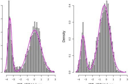
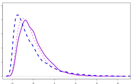
In light of the numerical outcomes from our Monte Carlo investigation, we plot three estimated density functions in Figure 3. The solid curves in each plot of Fig-ure 3 provide the kernel estimated density functions of the fecal and mucosal IPT-ICC

(31)

0.0 0.2 0.4 0.6 0.8 1.0 0 5 10 15 20 25 Density ICC Values (a) 0.0 0.2 0.4 0.6 0.8 1.0 0 5 10 15 20 Density ICC Values (b)

Figure 1: Histogram of ICC values. The density of the fitted two-component beta mixture to the (a) fecal data and (b) mucosa data is superimposed.

values, respectively. The estimated density functions based on the normal-mixture models are given by the dashed lines. Finally, the estimated density function calcu-lated using the transformation theory give the estimated density functions of IPT-ICC values in the dotted lines, when the ICC values were fitted with beta-mixtures. Even though not perfectly, the kernel density estimates and the normal-mixture based estimates correspond roughly well with each other. However, the transformed beta-mixture based density estimates misfit the lower beta-mixture component for the mucosa data. For fecal data, this approach almost concluded that there was a single compo-nent – a feature which could not be clearly seen in Figure 1.

(32)

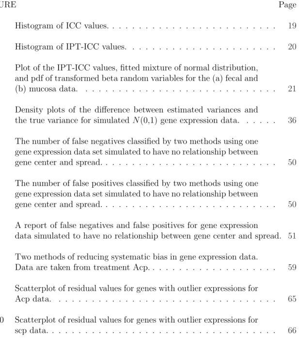
−4 −3 −2 −1 0 1 2 3 0.0 0.1 0.2 0.3 0.4 0.5 Density IPT−ICC Values (a) −4 −3 −2 −1 0 1 2 3 0.0 0.1 0.2 0.3 0.4 Density IPT−ICC Values (b)

Figure 2: Histogram of IPT-ICC values. The density of the fitted two-component normal mixture to the (a) fecal data and (b) mucosa data is superimposed.

3.4 Simulation Study

To investigate the fit of a beta mixture to probit transformed normal random variables and the fit of a normal mixture to inverse-probit transformed beta random variables, we conduct a Monte Carlo simulation study for each of the fecal and mucosa data sets. Our goal is to determine how well the densities fit data under model mis-specification. In other words, we want to assess the loss in accuracy if data is really normal but we transform and fit with beta or otherwise, if data is truly beta but we transform and fit with normal. Simulation for the fecal data is described as follows:

Simulation 1: Data Generated from Beta-mixtures, Fit with Normal-mixtures (1) Generate Y1, . . . , Yn from ˜fBf = 0.7 Beta(2.6,1.7) + 0.3 Beta(0.2,0.8).

(33)

−4 −2 0 2 0.0 0.1 0.2 0.3 0.4 Density Normal Beta Density IPT−ICC Values (a) −4 −2 0 2 0.0 0.1 0.2 0.3 0.4 Density Normal Beta Density IPT−ICC Values (b)

Figure 3: Plot of the IPT-ICC values, fitted mixture of normal distribution, and pdf of transformed beta random variables for the (a) fecal and (b) mucosa data.

(2) Transform Y1, . . . , Yn using the inverse-probit transformation and fit the

trans-formed data with a two-component normal mixture.

Simulation 2: Data Generated from Normal-mixtures, Fit with Beta-mixtures (1) Generate X1, . . . , Xn from ˜fNf = 0.7 N(0.04,0.80) + 0.3N(−3.5,0.07).

(2) Transform X1, . . . , Xn using the probit transformation and fit the transformed

data with a two-component beta mixture.

We repeat each simulation s=250 times for sample size n=1600 and use the EM algorithm to obtain estimates ˆθB and ˆθN. The steps above are repeated for

the mucosa dataset where the beta random variables are generated from ˜fm

B =

(34)

gener-ated from ˜fm

N = 0.8N(−0.30,0.60) + 0.2N(−3.3,0.10).

We could not compare the outcomes of Simulations 1 and 2 directly when the estimated parameters are for normal-mixtures and beta-mixtures, respectively. To ease the comparisons, we transform the resulting estimates in Simulation 2 so that the outcomes correspond to means and variances of distributions that would give observations on the whole real line.

Consider the following approach:

1. Retrieve (ˆαL,βˆL) and (ˆαU,βˆU) from the EM algorithm.

2. Generate 10,000 random variables from ZL ∼Beta(ˆαL,βˆL) and 10,000 random

variables from ZU ∼Beta(ˆα,β).ˆ

3. Transform ZL and ZU using the inverse-probit transform.

4. Calculate the mean and variance of the transformed random variables.

Steps 1-4 are repeated for each simulation.

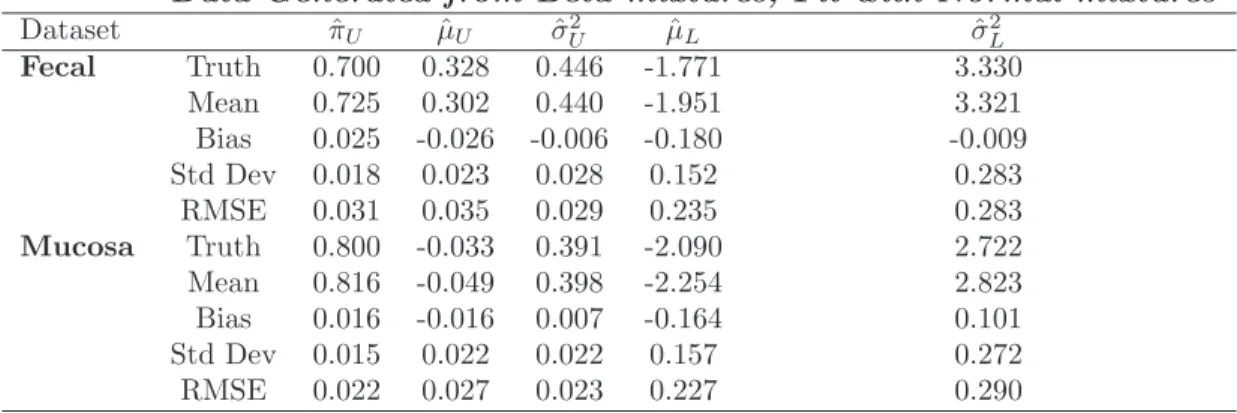
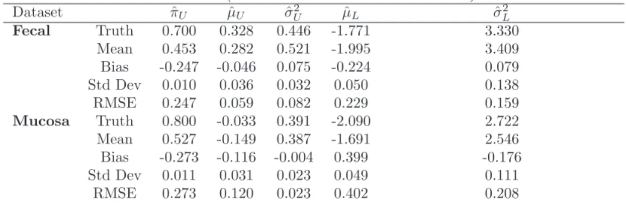
We present Monte Carlo statistics corresponding to the two components of the mixture distribution. Summary statistics for both simulation scenarios are presented in Table 1 and Table 2. We identify the target estimate of a scenario as ”Truth” and report Monte Carlo estimates of mean, bias, standard deviation, and the square root of mean squared error (RMSE).

When comparing the true estimates to those obtained from the fitted distribu-tion, we find that summary statistics from fitting transformed normal random vari-ables with a beta mixture closely resemble the phenomenon observed when analyzing the fecal and mucosa data. Namely, it is the case that although the true proportions for the upper components of the fecal and mucosa data are 0.7 and 0.8, respectively, estimates of πU resulting from the fit of a two-component beta distribution average

(35)

0.5. Moreover, the measure of bias in parameter estimation for fitting transformed normal random variables with a beta mixture is at least twice the bias in fitting transformed beta random variables with a normal mixture. This is true for almost every parameter estimation. These results lead us to believe that the two-component normal mixture is more robust to model mis-specification. Naturally, the normal mix-ture model fits normal data well. However, we also find that even if the data is truly beta distributed, we still retain significant accuracy if we alternatively transform the data into z-scores and fit with a normal distribution. On the other hand, assuming that the data is beta distributed could be costly if, in fact, it is not. We find that a biased conclusion could be reach if we model the two sets of ICC values using the mixture of betas.

Table 1: Monte Carlo mean, bias, standard deviation, and square-root MSE (RMSE) of estimates from simulation study ”Data Generated from Beta-mixtures, Fit with Normal-mixtures.”

Data Generated from Beta-mixtures, Fit with Normal-mixtures

Dataset πˆU µˆU σˆ2U µˆL σˆ2L Fecal Truth 0.700 0.328 0.446 -1.771 3.330 Mean 0.725 0.302 0.440 -1.951 3.321 Bias 0.025 -0.026 -0.006 -0.180 -0.009 Std Dev 0.018 0.023 0.028 0.152 0.283 RMSE 0.031 0.035 0.029 0.235 0.283 Mucosa Truth 0.800 -0.033 0.391 -2.090 2.722 Mean 0.816 -0.049 0.398 -2.254 2.823 Bias 0.016 -0.016 0.007 -0.164 0.101 Std Dev 0.015 0.022 0.022 0.157 0.272 RMSE 0.022 0.027 0.023 0.227 0.290

We further analyze the simulated outcomes and compare the sensitivity of each modeling approach toward distributional mis-specification through performing good-ness of fit tests against assumed models. Analysis of goodgood-ness of fit (Section 2.2.5) test statistics resulting from the simulation study are given in Table 3. Precisely, for each simulated data set, we let the null hypothesis, H0, be that the observed ICC (or

(36)

Table 2: Monte Carlo mean, bias, standard deviation, and square-root MSE (RMSE) of estimates from simulation study ”Data Generated from Normal-mixtures, Fit with Beta-mixtures.”

Data Generated from Normal-mixtures, Fit with Beta-mixtures

(beta estimates valued on real line)

Dataset πˆU µˆU σˆ2U µˆL σˆL2 Fecal Truth 0.700 0.328 0.446 -1.771 3.330 Mean 0.453 0.282 0.521 -1.995 3.409 Bias -0.247 -0.046 0.075 -0.224 0.079 Std Dev 0.010 0.036 0.032 0.050 0.138 RMSE 0.247 0.059 0.082 0.229 0.159 Mucosa Truth 0.800 -0.033 0.391 -2.090 2.722 Mean 0.527 -0.149 0.387 -1.691 2.546 Bias -0.273 -0.116 -0.004 0.399 -0.176 Std Dev 0.011 0.031 0.023 0.049 0.111 RMSE 0.273 0.120 0.023 0.402 0.208

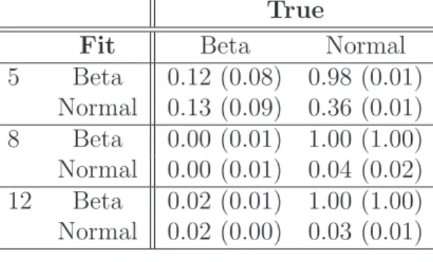
IPT-ICC) values are from the assumed model. We then compare the observed and the expected counts of observations within k bins, where k = 5, 8, 12, respectively, using Pearson’s chi-square goodness of fit tests with significance level α=0.05 and k−1 degrees of freedom. For large values of the test statistic, namelyX2 _{> χ}2

0.05,k−1, we reject the null hypothesis that the data comes from the assumed distribution.

Ideally, if the H0 is true, there should be no more than 5% chance to reject the H0 when α=0.05. Except for when k = 5, the proportion of tests that reject H0 with normal-mixture modeling are all less than nominal level of 0.05. Further, in all cases, the outcomes obtained by normal-mixture modeling are comparable to those obtained when the true underlying distributions are assumed. The same does not hold for beta-mixture modeling. When the data are not generated according to the beta-mixture scheme, the goodness of fits tests are rejected close to or equal to 100% throughout. That is, the best fits of beta-mixtures still could not provide sufficiently close approximations that could pass the goodness of fit tests under Simulation 1.

(37)

Table 3: P(X2 _{> χ}2

0.05,k−1) for fecal (mucosa) data using 5, 8, and 12 bins.

True

Fit Beta Normal

5 Beta 0.12 (0.08) 0.98 (0.01) Normal 0.13 (0.09) 0.36 (0.01) 8 Beta 0.00 (0.01) 1.00 (1.00) Normal 0.00 (0.01) 0.04 (0.02) 12 Beta 0.02 (0.01) 1.00 (1.00) Normal 0.02 (0.00) 0.03 (0.01)

3.5 ICC Comparisons of Fecal and Mucosa Data

Since our findings from the simulation study suggest that we use a two-component normal distribution to fit the probit transformed ICC values, we can accurately com-pare the fecal and mucosa array platform. In order to measure the quality of fecal array data, we first test for a distributional difference between ICC values from colon fecal and mucosa samples. With a p-value equating to 0, the likelihood ratio test (Section 2.2.6) rejects the null hypothesis. Thus, as expected, we deduce that the ICC values of genes obtained from the mucosa data are differentially expressed from those obtained from the fecal array data.

We further explore the extent of these distributional differences using bootstrap-ping for hypothesis testing. The first bootstrap analysis is designed to test for a differ-ence in the proportion of irreproducible genes contained in each data set. Specifically, we testHa:πF−πM 6= 0, whereπF andπM are the proportion of irreproducible genes

(genes with lower ICC values) in the fecal and mucosa data, respectively. Secondly, we determine whether there is a difference in the quality of information for reproducible genes. We test the hypothesis Ha:µF −µM 6= 0, whereµF and µM are means of the

upper mixture components for the fecal and mucosa data, respectively. Bootstrapped confidence intervals for the two respective tests are calculated to be (0.06,0.10) and

(38)

(0.27,0.40). As a result, we find that while the fecal array has a higher proportion of irreproducible genes, it averages ICC values for reproducible genes that are no worse than those obtained from the mucosa platform.

(39)

CHAPTER IV

VARIANCE ESTIMATION AND OUTLIER DETECTION METHODOLOGY

4.1 Introduction

Chapter IV is divided into two major components. First, we review variance esti-mation and introduce competing methodologies. Special focus is given to techniques which group genes in order to strengthen estimation. We discuss grouping G=50 genes to estimate variance. However, we also considered grouping 25 and 75 genes. While G=25 led to suboptimal power in detecting true outliers, there was no added benefit in G=75. Secondly, we give an overview of outlier detection algorithms.

4.2 An Overview of Variance Estimation

Microarray experiments are generally large in scale because a single array hybridiza-tion can generate thousands of data. However, since microarrays are costly and RNA samples are limited, replication of experiments is typically low in number. An issue of major concern in data analysis is the ability to estimate gene-specific variances from a small number of samples. Statistical tests such as the traditional t-test, which rely heavily on the sample variance, will have low power to detect differentially expressed genes if tests are carried out gene by gene. For example, a gene with small estimated variance could, by chance, have a large test statistic and be classified as differentially expressed even when the fold-change is small. This hinders the ability to draw reli-able biological conclusions. Previous work (Arfin et al., 2000) suggested estimating a global variance by pooling information across all genes. If variances are homogeneous across genes, then this is a suitable approach. However, this assumption is likely to be untrue since variation of expression levels are known to vary from gene to gene.

(40)

Various methods have been devised to stabilize gene-specific variances by bor-rowing information across genes. Alternative variance-stabilization approaches, such as the statistical analysis of microarrays (SAM) t-test (Tusher et al., 2001), adjust gene-specific variances by adding a small constant to each variance estimate. The methodology proposed by Baldi and Long (2001) assumes a dependent relationship between mean and standard deviation in array data and models the statistics jointly using a conjugate normal-inverse gamma prior distribution. Each estimate of variance is a weighted contribution of gene-specific and global variation. Lonnstedt and Speed (2002) formulate the B-statistic by using an empirical Bayes approach and combining information across many genes. Kendziorski et al. (2003) also use Bayesian techniques in their consideration of a hierarchical gamma-gamma model.

Using the idea that there are strengths in numbers, various approaches seek to im-prove variance estimation by grouping genes according to intensity values and apply-ing nonparametric smoothapply-ing techniques. Kamb and Ramaswami (2001) group genes by increasing average intensity and use regression to estimate gene-by-gene variance. Huang and Pan (2002) compare variance estimation obtained by (1) regression using equal weights, (2) loess regression giving less weight to more distant observations, and (3) nonparametric smoothing of the sample variance. Jain et al. (2003) propose local-pooled-error (LPE) estimation of within-gene expression error by pooling vari-ance estimates for genes with similar expression intensities as other gene expressions under the same experimental condition. Lin et al. (2003) use smoothed medians and smoothed MAD’s to estimate center and spread, respectively and construct stan-dardized test statistics. Comander et al. (2004) consider a different intensity-variation relationship and pool together variance estimates of genes with similar minimum in-tensity in hopes of pooling together genes that are likely to have similar variances.

(41)

dependency that has been observed in some microarray data. Rocke and Durbin (2001) assert that the variance of raw spot intensities increases with their mean and model intensities with a two-component model. Durbin et al. (2002) also develop an error model to quantify variance as a function of mean intensity. Based on the as-sumption of a quadratic relationship between center and spread, Huber et al. (2002) propose variance stabilizing methodology in order to stabilize variance at low inten-sities.

Two recent methodologies by Cui et al. (2005) and Tong and Wang (2007) make no presumptions about a variance-intensity relationship for microarray data and es-timate gene-specific variance components using shrinkage estimators. The method proposed by Cui et al. (2005) (referred to as the CHQBC estimator) presents esti-mates based on the James-Stein estimator (Lindley, 1962). Tong and Wang (2007) extend the shrinkage estimator methodology and suggest an optimal shrinkage pa-rameter to replace the James-Stein shrinkage factor. Throughout, we refer to this technique as the TW estimator.

We propose gene-specific variance estimates based on shrinkage estimation of ro-bust variance estimates. In the presence of outliers, performances of the CHQBC and TW methods deteriorate because each depend on the sample variance. To overcome this drawback, our approach replaces the sample variance by a robust variance estima-tor. In order to present a baseline comparison, we compare our proposed methodology to one which uses grouped estimation of variance determined by robust standard de-viation of residuals (Motulsky and Brown, 2006). Both methods borrow information across genes in order to increase power. They are described in detail in sections 4.3.1 and 4.3.2.

It is our belief that grouping genes by similar intensities does not guarantee that data pooled together share similar variability. If this is true and grouped estimates

(42)

of variation are inaccurate representations of the observed variation for genes within that group, then any conclusions drawn will be misleading. Furthermore, we are likely to underestimate (overestimate) gene-specific variances for genes with high (low) variation. Our goal is to stabilize variance estimates in order to detect outliers, so that we can better quantify gene-specific variation in microarray data.

4.3 Variance Estimation Methodologies

We describe leading variance estimation techniques, and variants thereof, in the sub-sections to follow.

4.3.1 Grouped Estimation of the Robust Standard Deviation of the Residuals

Motulsky and Brown (2006) consider a robust non-linear regression setting and use residuals of the curve fitting to estimate variance. Since it is expected that 68.27% of the values in a Gaussian distribution fall within one standard deviation of the mean, Motulsky and Brown quantify variation in the residuals by calculating the 68.27 percentile of the absolute values of the residuals. The robust standard deviation of the residuals (RSDR) has a breakdown point of 32%.

Rather than use all the data in a large-scale microarray expression data set, we propose an alternative method based on local grouped estimation of the RSDR (gr-pRSDR). Under an ideal setup we should have that each gene expression is scattered around its median expression value. Thus, residuals are computed from subtracting a gene’s median from its expression value. The steps for computing grpRSDR are:

1. Pool data by grouping 50 genes together and let I be the number of groups; I = G/50.

2. RSDRi = the 68.27th percentile of absolute residuals obtained from gene

(43)

Thus, the grpRSDR estimation of variance for genes g in groupi is given byRSDRi.

4.3.2 Tong & Wang’s Optimal Shrinkage Estimation of Variance

In order to estimate variance, we adopt Tong and Wang’s procedure for optimal shrinkage variation estimation (Tong and Wang, 2007). They propose a shrinkage estimator for gene-specific variance components which borrows information across variances.

4.3.2.1 Gene-specific Variance Estimation

Let Xg be the residual sum of squared errors (SSE) and σg2 be the true variance of

gene g. It is assumed that Xg/σg2 are independent and Chi-square distributed with ν

degrees of freedom, for g = 1, . . . , G genes. Thus, Xg ∼σ2gχ2ν.

After natural logarithmic transformation on Xg, the above expression is equivalent

to the following location model:

X_g0 =ln σ_g2+²0_g, (4.1) where X0

g =ln(Xg/ν)−m, ²0g =ln(χ2ν/ν)−m , and m=E(ln(χ2ν/ν)).

Cui et al. (2005) extend Stein’s theory for estimation of multiple means to mul-tiple variances and use the James-Stein shrinkage estimator to shrink the variance component of each gene towards the bias corrected geometric mean of variances. The James-Stein shrinkage estimator of ln σ2

g is given by ¯ X0 ₊ Ã 1− P(G−3)V (X0 g−X¯0)2 ! + (X0 g−X¯0), (4.2)

with shrinkage factor ¡1−(G−3)V /P(X0

g−X¯0)2

¢

+. The estimator is proven to have uniformly smaller mean square error than the maximum likelihood estimator. It

(44)

also requires no assumptions about the distribution of variances across genes. How-ever, the authors do note that the sampling distribution of the logarithm of variance estimates is assumed to be normal.

The CHQBC estimate of σ2

g that Cui et al. (2005) propose emerges upon

trans-forming (4.2) back to the original scale. We have that, ˜ σ2 g = ( G Y g=1 (Xg/ν)1/G) B×exp "µ 1− P (G−3)∗V (ln Xg −ln Xg)2 ¶ + ×(ln Xg−ln Xg) # , (4.3) whereV =var(²0 g),ln Xg = P_G

g=1ln(Xg)/GandB =exp(−m). If we letZg =Xg/ν, Zpool = Q_G g=1Z 1/G g , and ˆα0 = 1−(1−(G−3)V / P (ln Xg−ln Xg)2)+. Withα = ˆα0,

the CHQBC estimator may be written as ˜

σ2

g(α) =B(Zpool)α(Zg)1−α. (4.4)

Tong and Wang revise (4.4) by combining two unbiased estimators of σ2

g. If

variance homogeneity holds, then σ2

g =σ2 for all g, E(Zpool) = σ2/B, and BZpool is

an unbiased estimator of σ2

g. It is also the case thatZg is an unbiased estimate of σg2.

Hence, they present the following modification ˆ

σ2

g(α) = (BZpool)α(Zg)1−α, 0≤α≤1. (4.5)

The estimator ˆσ2

g is referred to as the TW estimator.

4.3.2.2 Estimation of the Shrinkage Parameter

In lieu of the shrinkage factor given in (4.2), Tong and Wang (2007) derive optimal estimation of the shrinkage estimator α. We implement the authors’ adaptation of optimization under the Stein loss function. The Stein Loss function,

(45)

converges to infinity as ˆσ2 _{approaches zero and as ˆ}_σ2 _{approaches infinity. Thus, gross} overestimation and underestimation of the true variance are equally penalized.

The authors present a family of shrinkage estimators for (σ2

g)t given by ˆ σ2_gt(α) = (hG(t)Zpoolt )α (h1(t)Zgt)1−α, 0≤α ≤1, (4.7) where hn(t) = ( ν 2) t µ Γ(ν 2) Γ(ν 2 + nt) ¶n (4.8) and Γ(·) is the gamma function. It is the case that whent = 1 and G is large, (4.7) reduces to (4.5).

The optimalαunder Stein loss function minimizes the average risk for each gene, which is given by R(σ2t_,_σ_ˆ2t_{) =} 1 G G X g=1 E(L(σ2t g ,σˆg2t)) = h α G(t)h1−1 α(t) hG−1 1 (αtG)h1((1−α+Gα)t) (σ_pool2 )αt1 G G X g=1 (σ_g2)−αt −ln (hα G(t)h1−1 α(t))−tΨ( ν 2) +tln ( ν 2)−1, (4.9) where t > ν/2, Ψ(t) = Γ0_{(t)/Γ(t) is the digamma function. The optimal estimator is} denoted as ˆσ2

Z,g(α∗1), where α∗1 = argmin

αε[0,1]

R(σ2t_,_σ_ˆ2t_).

4.3.2.3 Some Important Algorithm Details

In order to obtain an estimate of the optimal shrinkage parameter, it is necessary to assume that Zg → σg2 a.s. Let b(σ2) = (σpool2 )αtG1

P_G

g=1(σg2)−αt. Then we can

estimate b(σ2_{) with}_b(_Z_{) in (4.9). For small}_{ν, we also find it necessary to implement} an alternative two-step procedure:

1. Estimate b(σ2_{) with} _b(_Z_{) in (4.9) and compute a temporary optimal shrinkage} parameter and resulting temporary optimal shrinkage estimators, ˆσ2

(46)

2. Substitute b(σˆ2

∗) for b(σ2) in (4.9) in order to find the final optimal shrinkage parameter and estimators.

As the authors suggest, we truncate the smallest 1% of Zg’s in the procedure so that

estimation ofαremains stable. We use the built-in optimization code ’nlminb’ within the R computing environment to estimate α.

4.3.3 Proposed New Methodology: TW(mix/mad)

When outliers are present in the data, the gene-specific estimator of variance that Tong and Wang propose is prone to inaccurate estimation. The estimator relies heavily on the sample variance, which overestimates variance when the data is con-taminated by outliers. Alternatively, we propose to replace Zg in (4.7) with a vector

of robust variance estimates. The square of the median absolute deviation (MAD) would be a natural consideration for robust estimation of variance, but this statistic alone is insufficient. MAD has a tendency to underestimate standard deviation even when no outliers are present and could potentially create a problem with high counts of false positives. Our alternative uses information in the MAD and sample standard deviation to find the best variance estimate for a given gene.

To estimate the likelihood of an outlier in each gene’s expression data, we assess the relative change in standard deviation between an estimate robust to outliers and one influenced by outliers. Let

rg =

Sg −MADg

MADg

, (4.10)

where Sg and MADg are the sample standard deviation and MAD, respectively, of

gene g. The MAD is defined to be

(47)

where k ≈ 1.4826 for normally distributed data, unless otherwise stated. We will observe small values of rg when there is little deviation between MAD and sample

standard deviation, which suggests that the gene data may be free of outliers. On the other hand, we expect to observe large values ofrg for genes with significant outlying

expressions.

We consider shrinking the following vector of variance estimates: Vg =      1 2(Sg2+MAD2g) ifrg <= R MAD2 g if rg > R. (4.12) In order to specify the cutoff for the piecewise function, and also to justify why we choose to send Vg into Tong and Wang’s optimal shrinkage algorithm, we use the

following illustration: Simulate n=6 random observations from aN(0,1) distribution for G = 10,000 genes. Possible values of R were determined by percentiles of rg

ratios obtained from the simulated data. We ultimately chooseR=3.6, which was the approximated 99th _{percentile of}_r

g ratios. For all genesg withrg values exceeding 3.6,

we avoid any sensitivity to outlier observations since the relative change in variation is large. Instead, we quantify variation solely using the square of the MAD statistic. On the other hand, for all genes g withrg values at most 3.6, we send into the algorithm

the average of sample variance and the square of the MAD statistic.

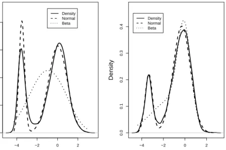
Ideally, we want to shrink estimates of variance which are not already believed to be distorted. In Figure 4, we plot the distribution of deviance from the true variance when using the square of the MAD statistic, the sample variance, and also, the average of the two to estimate variance. When there are no outliers in the data, the sample variance is most centered at zero deviation. We retain most of the same accuracy even when using the average of the sample variance and the square of the MAD statistic. However, the square of the MAD statistic is shown to consistently underestimate the true variance. For this reason, we choose not to rely solely on

(48)

the square of the MAD statistic in computing optimal shrinkage variance estimators. Certainly the sample variance will overestimate variance in the presence of outliers; however, the MAD statistic underestimates variance even when the data is free of outliers. By using the average of the two, we are able to protect against extreme overestimation and underestimation of the true variance. Thus, we derive Vg as the

population of variance estimates we wish to shrink.

−1 0 1 2 3 4 0.0 0.2 0.4 0.6 0.8 1.0

Deviance from True Variance

Density

Figure 4: Density plots of the difference between estimated variances and the true variance for simulatedN(0,1) gene expression data. Variance is estimated using three statistics - (1) square of the MAD statistic (dashed line), (2) sample variance (solid line), and (3) the average of sample variance and the square of the MAD statistic (dotted line).

The optimal shrinkage estimators based on our proposed methodology arise natu-rally after substituting b(V) forb(Z) in estimatingb(σ2_{) (section 4.3.2.3). We denote} these optimal shrinkage estimators as ˆσ2

(49)

estimate.

4.3.3.1 Grouped Estimation of TW(mix/mad) Methodolgy

As an extension of the previous section, we suggest further stabilizing variance es-timation by grouping together residuals that are standardized with robust optimal shrinkage variance estimators, ˆσ2

V,g (Section 4.3.3). The estimate of common variance

measures grouped estimation of the robust standard deviation of the standardized residuals (RSDSR). Because standardized residuals follow an approximately stan