Filippone, M., and Sanguinetti, G. (2011)
Approximate inference of the
bandwidth in multivariate kernel density estimation.
Computational
Statistics and Data Analysis, 55 (12). pp. 3104-3122. ISSN 0167-9473
http://eprints.gla.ac.uk/56330
Approximate Inference of the Bandwidth in
Multivariate Kernel Density Estimation
Maurizio Filipponea, Guido Sanguinettib a
University College London - Department of Statistical Science, 1-19 Torrington Place, London, WC1E 7HB.
b
University of Edinburgh - School of Informatics, Informatics Forum 10, Crichton Street, Edinburgh, EH8 9AB.
Abstract
Kernel density estimation is a popular and widely used non-parametric method for data-driven density estimation. Its appeal lies in its simplicity and ease of implementation, as well as its strong asymptotic results regarding its con-vergence to the true data distribution. However, a major difficulty is the setting of the bandwidth, particularly in high dimensions and with limited amount of data. An approximate Bayesian method is proposed, based on the Expectation-Propagation algorithm with a likelihood obtained from a leave-one-out cross validation approach. The proposed method yields an it-erative procedure to approximate the posterior distribution of the inverse bandwidth. The approximate posterior can be used to estimate the model evidence for selecting the structure of the bandwidth and approach online learning. Extensive experimental validation shows that the proposed method is competitive in terms of performance with state-of-the-art plug-in methods.
Keywords: kernel density estimation, Bayesian inference, expectation
propagation, multivariate analysis
1. Introduction
The estimation of a probability density function from a data set is an important statistical problem as it can provide useful insights on the prop-erties of the system from which data are observed, and can form the basis
Email addresses: [email protected](Maurizio Filippone),
for supervised and unsupervised learning steps. Non-parametric approaches make no assumption about the form of the density to be estimated, and the aim is to obtain an empirical estimate from the data which can provably con-verge (in a suitable sense) to the true data generating density in the limit of infinite sample size. A popular and widely used technique for non-parametric density estimation is Kernel Density Estimation (KDE) (Silverman, 1986). In KDE a base (also known as kernel) function K(x|λ) parametrized by a shape parameterλis selected, and the density is estimated as a superposition of kernel functions centered at the data points:
ˆ p(x) = 1 n n X j=1 K(x−xj|λ), (1)
where X = {x1, . . . ,xn} is a set of observed data points in Rd. The kernel function is a proper density function, thus guaranteeing that the estimate is an acceptable probability density. A common choice for the kernel function is the Gaussian kernel,
K(x|λ) = λ 2π d/2 exp −λ 2kxk 2 .
In this case, the parameterλis the precision of the Gaussian kernel and is the inverse of the square of the so calledbandwidthσ, namelyλ= 1/σ2. It can be shown that the KDE estimate of a probability density function converges, in terms of integrated squared error, to the true density in the limit of infinite data, while simultaneously shrinking the bandwidth (Silverman, 1986).
In practical situations, when the amount of data is finite, the bandwidth is a parameter that needs to be properly tuned to guarantee a good performance (Jones, 1991; Hazelton and Turlach, 2007). Several approaches have been proposed to estimate it (Cao et al., 1994; Jones et al., 1996; Silverman, 1986). The quality of a bandwidth selector is usually evaluated on the basis of the Integrated Square Error (ISE)
ISE =
Z
Rd
[p(x)−pˆ(x)]2dx (2) or its expectation (MISE). The direct optimization of any of these functions, or an asymptotic expansion of the MISE, requires some knowledge about the true density, that is usually unknown. Many bandwidth selectors are there-fore designed to optimize them by plugging in some estimates of the missing
characteristics of the true density (Loader, 1999; Sheather and Jones, 1991; Terrell, 1990; Duong and Hazelton, 2005; Chiu, 1991; Hall, 1982; Jones and Henderson, 2009). Some probabilistic approaches based on a maximum like-lihood (ML) approach have been proposed, where the probability of the data itself under the KDE estimate (1) is used as the likelihood. To deal with the unbounded likelihood when σ approaches zero, cross-validated or penal-ized forms of the likelihood have been considered (Silverman, 1986; Zhang et al., 2006). In Zhang et al. (2006, 2009), the cross-validated likelihood is used along with a prior on the bandwidth to sample from its posterior dis-tribution using Markov chain Monte Carlo (MCMC) methods. It is worth noting that this approach allows to deal with multivariate data in the same way it does with univariate data, as it is a likelihood-based approach. Other Bayesian approaches can be found in Brewer (2000), where an approach to Bayesian local smoothing for univariate data is considered; in particular, the bandwidth is locally adjusted to reflect the local density of the data. Also, Gangopadhyay and Cheung (2002) and de Lima and Atuncar (2011) provide closed form expressions for posterior densities over the bandwidth for uni-variate and multiuni-variate data respectively, but the likelihood used in these approaches is not the probability of the observed data given the bandwidth. Note that in the particular case of censored data the inference of the band-width can be done in closed form (Kulasekera and Padgett, 2006). Also, recent advances in multivariate KDE can be found in Tran et al. (2006); Duong et al. (2008).
In this paper, we propose an approximate Bayesian approach to the esti-mation of the bandwidth for KDE, where the kernel function is the Gaussian density. We place a prior distribution on the kernel precision (inverse band-width), and obtain a joint likelihood by combining the prior with an approx-imate likelihood obtained from leave-one-out cross-validation (van der Laan et al., 2004; Zhang et al., 2006). This yields a posterior distribution over the inverse bandwidth up to a proportionality constant. We propose a method to approximate the posterior that directly interprets the joint likelihood as
a cavity distribution, leading to a simple application of the
Expectation-Propagation (EP) algorithm (Minka, 2001; Opper and Winther, 2000). The motivation for a Bayesian approach is that it has many useful prop-erties. In particular, obtaining a posterior distribution over the bandwidth allows to quantify the uncertainty on the estimate of the bandwidth, thus allowing to consider different scenarios when analyzing data. If KDE is em-ployed as the first step of a supervised/unsupervised learning problem, such
as, e.g., Filippone et al. (2010); Rinaldo and Wasserman (2010), then a dis-tribution of decision functions can be obtained. Also, online learning can be approached quite naturally, as the posterior can be used as a prior when new data are observed. Finally, this provides a principled way to select the covariance structure for the bandwidth, namely full, diagonal, or isotropic, as the model evidence can be used to estimate Bayes factors (Kass and Raftery, 1995).
Although these are main reasons why one would consider a Bayesian ap-proach, most of these aspects have been overlooked in previous studies on KDE (Zhang et al., 2006, 2009). One of the contributions of this paper is to study, through extensive experiments, how the Bayesian approach can be used to select the structure of the bandwidth in multivariate KDE and per-form online learning. The main contribution is to present an approximate method to infer the bandwidth. In general, it can be argued that approxi-mate methods could lead to very poor approximations of the posterior distri-bution, especially in cases of multimodalities or inadequate assumptions on the approximating distribution. MCMC methods would therefore seem to be more flexible. However, especially in multivariate cases, the application of MCMC methods can be rather challenging. Designing efficient MCMC methods for sampling multivariate variables, ensuring good independence between samples and with a reasonable computational cost requires some fine tuning. For example, in the Metropolis-Hastings method (Metropolis et al., 1953; Hastings, 1970) it is required to specify the parameters of a proposal distribution, or in Hamiltonian-based Monte Carlo methods (Neal, 1993) the mass matrix. Also, assessing the convergence of MCMC methods or deal with multimodal posterior densities usually involves the running of multiple chains, as discussed, e.g., in Gelman and Rubin (1992); Kass et al. (1998); Calderhead and Girolami (2009). Clearly, these considerations imply a computational overhead that has to be accounted for in the design of an inference method. In the inference of the bandwidth in KDE, we found that the proposed approximate method yields a posterior density that is very close to the true one. Given the speed of the deterministic approximation scheme compared to MCMC methods, we propose it as an efficient alternative to in-fer the bandwidth in multivariate KDE. The advantages of the deterministic approximation through EP are that convergence can be monitored during the optimization and that the model evidence is readily available at the end of the algorithm. MCMC estimates of the model evidence, instead, could be rather challenging as discussed e.g., in Friel and Pettitt (2008) and Skilling
(2006).
The paper is organized as follows. In Section 2 we introduce the ideas underlying the Bayesian approach to multivariate KDE with a full preci-sion matrix, and in Section 3 we present the approximation of the posterior based on EP. In Section 4 we illustrate how to extend our method to online learning scenarios, while in Section 5 we give some details of implementation along with a discussion on the use of simpler structure for the precision ma-trix. Section 6 reports an extensive experimental comparison showing the performance of the proposed method, and Section 7 concludes the paper. In Appendix A, we detail the derivation of the special cases of diagonal and isotropic precision matrices.
2. Bayesian KDE
We consider multivariate Gaussian kernels
K(x|Λ) = |Λ| 1/2 (2π)d/2 exp −1 2x TΛx ,
where Λ is the precision matrix (inverse bandwidth) capturing the correla-tions among dimensions. The estimated pdf in x∈Rd is therefore
ˆ p(x) = 1 n n X j=1 K(x−xj|Λ) = 1 n n X j=1 N(x|xj,Λ), (3)
whereN (x|xj,Λ) denotes a normal distribution with mean xj and precision matrix Λ. Assuming i.i.d. data, one can define the log-likelihood:
L = log[p(X|Λ,MX)] = n X i=1 log " n X j=1 N (xi|xj,Λ) # + const.,
whereMX denotes the fact that the model is based on placing kernels at the data points in X. It can be easily seen, however, thatL is unbounded in Λ, achieving infinite value when the determinant of Λ goes to infinity.
In order to overcome this limitation, while retaining a ML approach, it has been proposed to maximize a cross-validated type of likelihood (Silverman, 1986) Lcv = log[p(X|Λ,MX)] = n X i=1 log " n X j6=i,j=1 N(xi|xj,Λ) # + const.. (4)
Provided xj 6=xi∀i, j, Lcv is a well behaved function of Λ and will be used in the remainder of this paper as the likelihood in the inference problem. Note that the definition in (4) does not define a proper joint probability distribution over X, as it is a mixture of degenerate distributions. In the case of ties instead, namely when xj = xi for some i 6= j, it is possible to use ideas from ˙Zychaluk and Patil (2008), where theoretical studies are reported on the asymptotics of estimates of the bandwidth based on the cross-validation method for minimizing the ISE (Hall, 1982).
To cast the problem in a Bayesian framework, we need to place a prior over the precision matrix Λ. To exploit conjugacy with the Gaussian kernel, we will use a Wishart prior
p(Λ) =W(Λ|Λ0, ν0) ∝|Λ|ν20− d+1 2 exp −1 2Tr(Λ −1 0 Λ) . (5)
In absence of prior knowledge about the bandwidth to use, we can use an uninformative improper Wishart prior p(Λ) = |Λ|−d+12 or a reasonably flat
Wishart prior, for instance, by setting ν0 =d+ 1 and Λ0 =βI with largeβ. The posterior is then
p(Λ|X,MX)∝p(X|Λ,MX)p(Λ), and the so called model evidence is
p(X|MX) =
Z
p(X|Λ,MX)p(Λ)dΛ.
The model evidence gives the probability of the observed data given the model assumption only, as the parameters are integrated out, and can there-fore be used for model selection. Given the complex analytical form of the likelihood, exact inference of Λ is intractable. In the next section we will show an approximation method based on EP.
The approximate inference process leads to a deterministic approximation of the posterior distribution over Λ and therefore allows to estimate the model evidence. Model comparison can be done using the so called Bayes factor
(Kass and Raftery, 1995) that is computed as the ratio between the evidence for the two models to compare. In Bayesian KDE, we can use this idea to compare different multivariate structures of the bandwidth, thus having a principled way of choosing whether simpler structures can be used in place of more complicated ones.
3. Expectation Propagation Estimation of the Bandwidth 3.1. Expectation Propagation
We briefly review here the EP algorithm (Minka, 2001; Opper and Winther, 2000); for more details see e.g. Bishop (2007). Consider a data modeling problem, where the observed data is denoted by X and the set of model parameters is θ ∈ Θ. EP aims at finding an approximation q(θ) to the pos-terior p(θ|X) by minimizing of the Kullback-Leibler divergence between the posterior and the approximating distribution:
KL[p(θ|X)||q(θ)] = Z Θ log p(θ|X) q(θ) p(θ|X)dθ.
It can be easily shown that this is equivalent to matching the moments be-tween the two distributions.
Generally, the direct computation of the moments of the posterior is in-tractable, and an iterative procedure for matching the moments is necessary. In the case of i.i.d. data, the posterior distribution over the parameters factorizes as p(θ|X) = 1 Z n Y i=0 fi(θ),
where f0(θ) is the prior and fi(θ) is the likelihood of the i-th observation. Let the approximating distribution q(θ) factorize as a product of tractable distributions: q(θ) = 1 ˜ Z n Y i=0 ˜ fi(θ). The goal is to optimize
KL " 1 Z n Y i=0 fi(θ) 1 ˜ Z n Y i=0 ˜ fi(θ) #
with respect to the approximating distributions ˜fi. In order to do that, we start from the so called cavity distribution, where we remove the j-th factor from q(θ) q\j(θ)∝ n Y i6=j,i=0 ˜ fi(θ),
and match the moments of the normalized version of fj(θ)q\j(θ) andqnew(θ). Once we have a revised version ofqnew(θ), we can obtain the updated version of ˜fj(θ) as
˜
fj′(θ)∝ qnew(θ)
q\j(θ) .
Starting from an initialization of the factors ˜fi(θ), we can update them in turn until convergence (Minka, 2001). In many occasions, EP has been used to ap-proximate the posterior using a Gaussian distribution (Opper and Winther, 2000). In our problem, since the bandwidth is constrained to be positive definite, such an approximation would not be acceptable. Therefore, we will model the factors as Wishart distributions.
Matching the moments of Wishart distributions would require matching the normalization constant, the mean, and the expectation of log|Λ|. The resulting equation for log|Λ|, however, cannot be solved analytically and requires an iterative optimization method. For simplicity, we will therefore pursue an approximation of the moment of second order (variance) based on the squared Frobenius norm
kΛk2
F = Tr(ΛΛT) =
X
ij
(Λij)2.
3.2. EP approximation of the posterior of the bandwidth of the kernel
In this section, we present the application of the EP framework for the ap-proximation of the posterior distribution over the precision. In order to keep the notation uncluttered, we define the unnormalized Wishart distribution as ˜ W(Λ|Λi, νi) = |Λ| νi 2− d+1 2 exp −1 2Tr(Λ −1 i Λ) .
The normalized Wishart distribution, instead, is defined as
W(Λ|Λi, νi) =BW(Λi, νi) ˜W(Λ|Λi, νi), with BW(Λi, νi)−1 = 2 νid 2 |Λ i| νi 2 π d(d−1) 4 d Y i=1 Γ νi+ 1−i 2 .
The true posterior is
p(Λ|X,MX)∝ n
Y
i=0
where f0(Λ) = W(Λ|Λ0, ν0) denotes the prior, and the components fj(Λ) read: fj(Λ) =p(xj|Λ,MX) = 1 n−1 n X r6=j,r=1 N(xj|xr,Λ).
We propose to approximate the posterior over Λ as
q(Λ) = n Y i=0 ˜ fi(Λ).
We consider an approximating form in which the factors are proportional to an unnormalized Wishart distribution
˜
fi(Λ) =γiW˜(Λ|Λi, νi),
with ˜f0(Λ) =f0(Λ). With this choice, it can be easily verified that
q(Λ) = n Y i=0 γi ! ˜ W Λ ( n X i=0 Λ−i 1)−1, n X i=0 νi−(d+ 1)n ! .
The cavity distribution, when we remove the j-th component fromq(Λ) is
q\j(Λ) = n Y i6=j,i=0 ˜ fi(Λ) = n Y i6=j,i=0 γi ! ˜ W Λ ( n X i6=j,i=0 Λ−i 1)−1, n X i6=j,i=0 νi−(d+ 1)(n−1) ! . (6)
Let’s define the following quantities: (Ur)−1 = n X i6=j,i=0 Λ−i1+ (xr−xj)(xr−xj)T, (7) α= n X i6=j,i=0 νi−(d+ 1)(n−1) + 1, (8) ψ = n Y i6=j,i=0 γi ! 1 (n−1)(2π)d/2, (9)
zr =BW(Ur, α)−1. (10) With the above definitions, we see that
fj(Λ)q\j(Λ) =ψ n
X
r6=j,r=1
zrW(Λ|Ur, α). (11)
Now we have to match the moments of
q(Λ|Λnew, νnew) = γnewBW(Λnew, νnew)−1W(Λ|Λnew, νnew)
with those of fj(Λ)q\j(Λ). The normalization constant of (11) is
E0 = Z fj(Λ)q\j(Λ)dΛ =ψ n X r6=j,r=1 zr. (12)
The mean and the variance of fj(Λ)q\j(Λ) can be computed noticing that the resulting density is a weighted sum of Wishart
fj(Λ)q\j(Λ)∝ n
X
r6=j,r=1
wrW˜(Λ|Ur, α),
where the weights are
wr =
zr
Pn
s6=r,s=1zs .
Therefore, the expectation results in
E1 = Efj(Λ)q\j(Λ)[Λ] =α n
X
r6=j,r=1
wrUr. (13)
The variance of Λ can be easily computed, given that Efj(Λ)q\j(Λ)[Λ2lk] = n X r6=j,r=1 wr (α+α2)(Ur)2lk+α(Ur)ll(Ur)kk . Therefore, E2 = var(Λ) = n X r6=j,r=1 wr (α+α2)kUrk2F+α[Tr(Ur)]2 − kE1k2F. (14)
Matching the moments results in:
γnewBW(Λnew, νnew)−1 =E0,
νnewΛnew =E1,
νnewkΛnewk2F+νnew[Tr(Λnew)]2 =E2,
that can be solved with respect to νnew, Λnew, and γnew, obtaining:
νnew = kE1k2F+ [Tr(E1)]2 E2 , (15) Λnew= E1 νnew , (16)
γnew=E0BW(Λnew, νnew). (17)
The updated version of ˜fj(Λ) is the ratio betweenq(Λ|Λnew, νnew) andq\j(Λ), resulting in ˜ fj′(Λ) =γj′W˜(Λ|Λ′j, νj′), where γj′ = Qnγnew i6=j,i=0γi , (18) Λ′j−1 = Λ−new1 −( n X i6=j,i=0 Λ−i 1)−1, (19) νj′ =νnew− n X i6=j,i=0 νi+n(d+ 1). (20) When the moment matching procedure satisfies a predefined convergence criterion, the resulting approximating posterior is
q(Λ) = γW˜(Λ|Λ, ν),
that allows to obtain the approximate model evidence as evidence =γ BW(Λ, ν)−1.
4. Online Bayesian KDE
Online learning arises quite naturally in Bayesian inference. In our case, let’s assume that the posterior over the precision, after having observed a data set X = {x1, . . . ,xn}, has been approximated using EP. This means that we have an approximation top(Λ|X,MX) based on a model MX where X is the set of centers of the kernels. When we observe new data, and we want to include them in the inference of the bandwidth, we need to extend the model to account for the new centers of the kernels. In particular, the final goal will be to approximate p(Λ|X, Y,MX∪Y) starting from p(Λ|X,MX).
Let’s analyze the following expression of the posterior:
p(Λ|X, Y,MX∪Y)∝p(Y|Λ,MX∪Y)p(X|Λ,MX∪Y)p(Λ).
We immediately see that this expression is based on a different model with respect to
p(Λ|X,MX)∝p(X|Λ,MX)p(Λ).
Therefore, the posterior p(Λ|X,MX) cannot be used directly as a prior for the second stage of inference. This problem, however, can be easily solved in the following way. First we need to extend the model from MX to MX∪Y. This can be done by approximating again p(Λ|MX∪Y) as a product ofn+ 1 factors p(X|Λ,MX∪Y)p(Λ)≃ n Y i=0 ˜ gi(Λ), where each factor is approximated by
˜ gj(Λ) = 1 n+m−1 (n−1) ˜fj(Λ) + n X r=1 N(xj|yr,Λ) ! ,
and ˜g0(Λ) is the prior. This approximation does not require operations among vectors in X, that were used to obtain the factors ˜fj(Λ). In practice, the first approximation stage yields
(n−1) ˜fj(Λ)≃ n
X
r6=j,r=1
N(xj|xr,Λ).
At the end of this stage, we have p(X|Λ,MX∪Y)p(Λ) as an unnormalized Wishart. Now we just need to include p(Y|Λ,MX∪Y) to obtain the updated
posterior. Given that p(Y|Λ,MX∪Y) = 1 n+m−1 n X r=1 N(yj|xr,Λ) + n X r6=j,r=1 N(yj|yr,Λ) ! ,
again we do not need to perform operations among vectors in X. Now the approximation to p(Λ|MX∪Y) will be a product of n+m+ 1 factors:
q(Λ|MX∪Y) = n+m Y i=0 ˜ fi(Λ) = n Y i=0 ˜ gi(Λ) m Y i=1 ˜ hi(Λ).
The first product is the Wishart obtained when we extended the model, so the final posterior is a product of m+ 1 factors. Again, we can employ an EP scheme to iteratively update the factors, obtaining an approximation to the posterior p(Λ|X, Y,MX∪Y).
5. Simpler structures of precision matrix and implementation de-tails
In this section we provide more details on how to implement the proposed method and we discuss how to reduce its complexity by considering simpler structures of precision matrix, namely diagonal and isotropic. The detailed derivation of these two special cases can be found in the appendix.
5.1. Implementation Notes
The presented method involves several matrix inversions. We can avoid them by working with the covariances Σi rather than the precisions Λi. In particular the computation of the matricesUr can be now simplified by using the Sherman-Morrison formula:
(Ur)−1 = n X i6=j,i=0 Σi+ (xr−xj)(xr−xj)T. Defining Q= n X i6=j,i=0 Σi !−1 , a=xr−xj, we obtain Ur =Q− QaaTQ 1 +aTQa. (21)
We report the pseudo-code of the proposed algorithm in Tab. 2; note that we actually work with the logarithm of the normalization constants of the Wishart distributions and the evidence by using standard log-sum and log-diff operations in order to avoid numerical underflows.
5.2. Reduced forms for precision matrix and complexity analysis
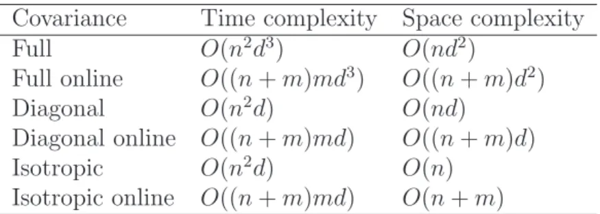
The inference of the full precision matrix can be computationally inten-sive. The reason is that each main iteration involves a loop ofniterations (for the refinement of thenfactors) each of which has time complexity inO(nd3). This complexity is dominated by the the computation of the normalization constants of the Wishart distributions with scale matrices Ur that involves the computation of |Ur| that has time complexity in O(d3). We notice that the complexity does not change even if we precompute and store the vectors
a in (21). In terms of spatial complexity, the dominant part is related to storing the matrices Λi and Ur that requires O(nd2).
As we have discussed in Section 4, the online version wherem new data point have to be included in the inference of the precision, does not require operations among the n data points used in the first part of the inference stage. We recall that the online version comprises two steps. In the first step we need to extend the model to include the new m data points; one main iteration of this step, involves a loop over n factors and requires the computation of m determinants |Ur|. Therefore, a whole iteration of the first step has time complexity O(nmd3). One main iteration of the second step, contains a loop of m factors only (as the other n are merged in one unnormalized Wishart), and again will be dominated by the computation of the determinants of |Ur|, yielding a time complexity in O(m2d3). For the space complexity, we can repeat the same considerations as in the offline case, accounting for the fact that we need to store the updated version of the
n matrices Λi computed in the first stage, leading to O((n+m)d2).
Due to the cubic scaling of the time complexity with respect tod, it might be useful to consider simpler forms of precision matrices, such as diagonal or isotropic. In particular, their respective forms are Λ = Iλ with λ =
(λ1, . . . , λd), and Λ = λI. In these cases, we place a Gamma prior over the precisions for each component λk for the diagonal precision, or a Gamma prior over the precision λ.
In the diagonal case, the time complexity of one iteration of the main loop is linear in the number of dimensions d, and is quadratic in n, leading to O(n2d). The size of the largest objects is in O(nd), as they are n ×d
Table 1: Time and Space complexity for one iteration (main loop) of the three versions of the approximate Bayesian KDE.
Covariance Time complexity Space complexity Full O(n2d3) O(nd2) Full online O((n+m)md3) O((n+m)d2) Diagonal O(n2d) O(nd) Diagonal online O((n+m)md) O((n+m)d) Isotropic O(n2d) O(n) Isotropic online O((n+m)md) O(n+m)
matrices. With the same considerations as in the full case, the online version has time complexity in O((n+m)md) and space complexity inO((n+m)d). In the isotropic case, in each iteration of the main loop we have to com-pute the distances between a data point and all the other n; this has time complexity in O(nd). Therefore, one of the main iterations will have a time complexity in O(n2d). The space complexity will be inO(n), as we will only need to allocate the vectors of sizen. It is interesting to notice that precom-puting the distances (time complexity inO(n2d), space complexity inO(n2)) will reduce the computational complexity in each main iteration to O(n2). Time and space complexities for the online versions follow straightforwardly as O((n+m)md) and O(n+m) respectively.
The complexity of one iteration for the three versions of the algorithm are summarized in Tab. 1. After extensive trials and evaluations, we noticed that a number of iterations in the order of tenths or sometimes less are needed for the proposed method to converge.
5.3. Initialization and Convergence
Denoting the parameters of the initializing posterior over Λ with γpost, Λpost, andνpost, in the case when we want to assign the same initial value to the Λi as well as to theνi, we get
n X i=0 Λ−i 1 = (Λpost)−1 ⇒Λ−i 1 = Λ−post1 n − Λ−01 n , n X i=0 νi−(d+ 1)n =νpost ⇒νi = νpost n − ν0 n +d+ 1,
n
X
i=0
log(γi) = log(γpost)⇒log(γi) =
log(γpost)
n −
log(γ0)
n .
In the experiments, we noticed that the initialization is usually not critical, in the sense that many different strategies lead to the same approximation. The former equations can be straightforwardly extended in the cases of diagonal and isotropic matrices.
As far as the convergence is concerned, we can monitor the change in the parameters of the approximating distribution. When these parameters change less than a threshold, we stop the iterations. In our experiments, we monitored the number of degrees of freedom, leading to the following convergence criterion:
|νnew−νold|< ε, with ε= 10−3.
We note here that Q in (21) is not positive semidefinite in general. In this case, the matrices Ur can have negative determinant and the whole procedure would fail to converge. This happens when few data are provided with respect to the dimensionality of the problem; in practice this means that the approximation using a unimodal Wishart is not suitable. We can fix this issue by increasing the diagonal elements of Q. In practice, we compute the smallest eigenvalue ofQ, and if it is negative, we subtract it to the diagonal of
Q. Given the form assumed by Q, we can view this operation as an increase in the prior covariance Σ0. When this happens, usually the model evidence penalizes the choice of this model.
6. Experimental Validation
In this section we present an extensive validation of our method. First we show the quality of the approximation of the posterior over the precision, and how the model evidence can be used to select the structure of precision matrix in multivariate cases. We then report a study on sampling techniques, comparing their running time with the proposed method. We also study the quality of the approximation in online and offline learning scenarios by comparing their approximate posteriors against the true one in a univariate problem. Finally, we show the performance in terms of ISE when we select the inverse of the expectation of the precision as the bandwidth, comparing it with state of the art methods for selecting the bandwidth, to demonstrate that the proposed method is competitive with the advantage of allowing
Table 2: Pseudo-code of the approximate Bayesian KDE algorithm.
1. set the maximum number of iterations maxit and the convergence pa-rameter ε
2. set the parameters ν0 and Λ0 of the prior
3. initialize the values of log(γi),νi, and Σi as explained in Section 5 4. for iin 1 : maxit
(a) for j in 1 :n
i. compute Ur for r = 1, . . . , n using (21)
ii. compute α, log(ψ), log(zr) for r = 1, . . . , n, using (8), (9), and (10)
iii. compute log(E0), E1, E2, using (12), (13), and (14) iv. compute log(γnew), νnew, Σnew, using (15), (16), and (17)
v. compute log(γ′
j), νj′, Σ′j, using (18), (19), and (20) (b) ifconvergence criterion is satisfied then exit the loop
online learning and model selection. All the algorithms have been run on a quad-core 2.66GHz Intel workstation with 8GB of RAM.
6.1. Quality of the posterior approximation
In this section, we report two illustrative examples to show the approxi-mation of the posterior over the precision in two synthetic cases; the first is a univariate problem, and the second one is bivariate.
6.1.1. Illustrative examples - Univariate and bivariate cases
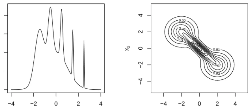
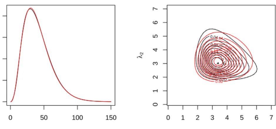
We considered a data set of 50 data points sampled from the univariate distribution in the left panel of Fig. 1. This problem has been studied in Marron and Wand (1992) where it is referred to the “asymmetric claw”. We numerically computed the actual posterior distribution as the multiplication of the prior (we chose a rather flat prior with a0 = 1, b0 = 0.01) and the likelihood, normalized to integrate to one (black curve in the left panel of Fig. 2). In the same figure, we show the approximation obtained by EP in red. The approximation of the posterior is quite accurate in capturing its expectation, variance, and log evidence. In the left panel of Fig. 3 we show in red the pdf when we selected the expectation of the precision, and in black
−4 −2 0 2 4 0.0 0.1 0.2 0.3 0.4 x p(x) x1 x2 0.01 0.02 0.03 0.04 0.05 0.06 0.07 0.08 −4 −2 0 2 4 −4 −2 0 2 4
Figure 1: Left: the “asymmetric claw” density function - Right: a bivariate pdf.
dashed lines the 5th and 95th percentiles of the pdfs values when sampling the precision from the posterior.
We considered the synthetic distribution in the right panel of Fig. 1, that is a mixture of three Gaussians (Duong and Hazelton, 2005). We sampled 200 data points from it and we ran our method to approximate the precision. We chose a diagonal structure for the precision matrix as it is easy to visualize the resulting posterior, and we chose a rather flat prior with parameters
a0k = 1,b0k = 0.01. Again, we numerically computed the actual posterior as the multiplication of the likelihood and the prior, normalized to integrate to one (black curve in the right panel of Fig. 2). In the same figure, we show the posterior approximation in red. As in the multivariate case, we see that the approximation captures the main characteristics of the posterior. In Fig. 3 we show in red the pdf when we selected the expectation of the approximate posterior over the precision in the two synthetic cases.
6.1.2. Model selection for choosing the structure of the precision matrix
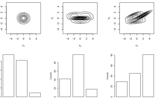
We considered the bivariate pdfs in the first row of Fig. 4, so that it is easier to interpret the results. We ran the approximate version of Bayesian KDE using the three forms of precision matrix, we computed their respective model evidence, and we used them to compute the Bayes factors to compare the models. When models M1 and M2 were compared, we chose model
0 50 100 150 0.000 0.010 0.020 λ p( λ |X ) λ1 λ2 0.02 0.04 0.06 0.08 0.1 0.12 0.14 0.18 0 1 2 3 4 5 6 7 0 1 2 3 4 5 6 7 0.02 0.04 0.06 0.08 0.1 0.12 0.14 0.18
Figure 2: Approximation of the posterior distribution over the precision. Left: univariate case - Right: bivariate case
−4 −2 0 2 4 0.0 0.1 0.2 0.3 0.4 0.5 0.6 x p(x) x1 x2 0.02 0.04 0.06 0.08 −4 −2 0 2 4 −4 −2 0 2 4 0.02 0.04 0.04 0.06
Figure 3: KDE densities when we select the precision as the expectation of the approxi-mated posterior. Left: univariate case, where the dashed lines represent the 5th and 95th percentiles of the values taken by the pdfs when sampling the precision from the posterior - Right: bivariate case
x1 x2 0.02 0.04 0.06 0.08 −4 −2 0 2 4 −4 −2 0 2 4 x1 x2 0.01 0.02 0.03 0.04 0.05 0.06 −4 −2 0 2 4 −4 −2 0 2 4 x1 x2 0.01 0.02 0.03 0.04 0.05 0.06 0.08 −4 −2 0 2 4 −4 −2 0 2 4
Iso Diag Full
Counts 0 20 40 60 80
Iso Diag Full
Counts 0 20 40 60 80
Iso Diag Full
Counts 0 20 40 60 80
Figure 4: First row: Three bivariate densities - Second row: Counts of how many times the three different models were selected in the three cases above.
3, that is a common rule for preferring a model over another (Kass and Raftery, 1995). We report a study of model selection for the distributions shown in Fig. 4, where we sampled 100 times a set of n = 100 data points from them. We ran the three algorithms considering the same flat prior, that is ν0 =d+ 1, Σ0 = 2I/10 for the Wishart, and a0 = 1, b0 = 0.1 for the Gamma. We counted the model with the largest evidence as well as those whose evidence is within a factor of 1/3 with respect to it. The results are reported in the second row of Fig. 4.
We can see that for the first pdf, on average, the isotropic precision is preferred as the problem is isotropic. In the second case, instead, the pdf is elongated along one of the axes, so a diagonal precision is selected more ofter than the isotropic and the full ones. Finally, the third case shows that a full covariance matrix is preferred by the Bayes factor when data have correlations between dimensions.
6.1.3. Comparison with sampling techniques
We compare our method with the one proposed in (Zhang et al., 2006), where Metropolis-Hastings sampling is used to sample from the posterior. In the case of a full precision matrix, the Authors consider the Cholesky decomposition
Λ =LLT,
where L is lower triangular. Using this factorization, the prior used in their experiment for the nonzero elements of L was
p(lij) = 1 1 +ρl2
ij ,
with ρ controlling the flatness of the prior. The likelihood is the cross-validated one in (4). As in Zhang et al. (2006), in all our experiments, we set ρ = 1, the number of burn-in samples to 5000, and the total number of samples to 25000. The parameters of the proposal were selected to keep the acceptance rate between 20% and 30%; this, of course, required few trials run that we have not accounted for in the comparison of running time, although they represent a cost in the whole inference process.
We studied the running time of EP and sampling methods in two cases. The first was the bivariate density in Fig. 1, and the second was a mixture of two Gaussians in 4 dimensions centered at (0,0,0,0) and (1,1,1,1) with identity covariance matrices. The ratio of running times for EP against sam-pling is reported in Tab. 3, where the algorithms have been run 10 times for each value of n. To ensure fair comparison, all the algorithms have been implemented in R (R Development Core Team, 2006). We can see how the
approximation is considerably faster than sampling. As a check, we also compared the performance in terms of likelihood of unseen data, finding that they were comparable (results not shown). In the case of a full covariance, in high dimensions and with a limited amount of data, we noticed that sampling techniques were superior in terms of performance, given that the approxima-tion of the posterior is not adequate. In these cases, a simpler covariance structure was favoured by Bayes factors. For the sake of brevity, we do not report comparisons in the case of simpler covariance structures; we just point out that the approximation is again considerably faster than sampling.
6.1.4. Online vs offline
We now show the quality of the approximation in an online scenario. We considered the univariate density in Fig. 1, from which we sampled 500 data
n = 200 n= 500 n = 1000
d= 2 0.10 0.15 0.16
d= 4 0.20 0.19 0.31
Table 3: Ratio between running times of the approximation method vs sampling. As a frame of reference, sampling in the case of d = 4 andn = 1000 took a couple of hours, and ford= 2 andn= 500 about 6 minutes.
20 40 60 80 20 40 60 80 True Expectation Expectation Offline 5 10 15 20 5 10 15 20 True St dev St de v Offline −770 −750 −730 −710 −770 −740 −710
True Log Evidence
Log Evidence Offline
20 40 60 80 20 40 60 80 True Expectation Expectation Online m=5 5 10 15 20 5 10 15 20 True St dev St de v Online m=5 −770 −750 −730 −710 −770 −740 −710
Log Evidence Online
Log Evidence Online m=5
20 40 60 80 20 40 60 80 True Expectation Expectation Online m=50 5 10 15 20 5 10 15 20 True St dev St de v Online m=50 −770 −750 −730 −710 −770 −740 −710
Log Evidence Online
Log Evidence Online m=50
Figure 5: Expectation and standard deviation of the posterior over the precision and log evidence of the model First row: offline vs true Second row: online (m = 5) vs true -Third row: online (m = 50) vs true.
points that we used to run the offline version of our method. In order to compare the inference results with online learning, we ran the offline version on half data only and then we ran two online versions adding m = 5 and
m = 50 data points at a time respectively. We compared the mean, variance, and log evidence of the true posterior against those of the approximations obtained by the offline and online versions (Fig. 5). We can see that the offline version is extremely accurate in capturing the moments of the posterior. The online versions do not differ very much from each other, and show an underestimation of the standard deviation; this is reasonable, given that the online version builds the solution upon an approximate form of the posterior obtained over the first batch of data. The evidence is still captured extremely well, while the expectation of the posterior is slightly underestimated on average.
6.2. Performance comparison 6.2.1. Synthetic data sets
50 100 200 500 1000 −5.5 −4.5 −3.5 −2.5 n log(ISE) n EP RT hpi hlscv hscv 100 200 500 1000 −7.5 −6.5 −5.5 −4.5 n log(ISE) n EP RT Hpi Hlscv Hscv
Figure 6: log(ISE) vsnover 100 repetitions for the univariate and bivariate data sets
In order to evaluate the performance of the proposed method, we carried out a study of the ISE in (2) with respect to the size of the data sampled from the true distribution. In particular, we sampled n data points from the true distribution and we estimated/inferred the bandwidth using several methods. Then, we computed the ISE score corresponding to the different
estimates of the density functions. We repeated this procedure for different values of n and 100 times for each value of n.
We compared EP with the following methods for bandwidth estimation: Silverman (1986) rule of thumb (RT), which is 1.06 min(sd(x),IQR/1.34)n−1/5
with IQR denoting the interquartile range; the plug-in (hpi) method of Wand and Jones (1994); least-squares cross-validation (hlscv) of Bowman (1984); and smoothed cross-validation (hscv) of Jones et al. (1991). In the
multi-variate case, RT corresponds to selecting a bandwidth for each covariate to be σi
h
4 (d+2)n
i1/(d+4)
, whereσi is the estimated standard deviation of thei-th covariate. The multivariate versions of hpi,hlscv, andhscvwill be denoted
asHpi,Hlscv, andHscv; Duong and Hazelton (2005) presented descriptions
of these methods and implementations can be found in the R packageks. We considered the synthetic distributions in Fig. 1. The results are shown in the plots in Fig. 6. We can see that the performance of the proposed method in terms of ISE is comparable to the best among the comparing methods. Note also that none of the considered bandwidth selectors is su-perior to the others in general, while the proposed method achieves an ISE that is often comparable to the best among the methods considered in the comparison.
6.2.2. Real data sets
We applied the proposed methods to three real data set(s): Old Faithful, Unicef, and Earthquake. In cases of ties, we simply added a uniform random contribution of the order of the least significant digits to resolve them.
Old Faithful data set. This is a one dimensional data set containing 107
eruption lengths of Old Faithful geyser in Yellowstone National Park.
Unicef data set. The Unicef data set has two covariates: the number of
deaths of children under 5 years of age per 1000 live births, and the average life expectancy (in years) at birth for 73 countries having gross national income less than $1000 per annum per capita.
Earthquake data set. This data set contains 510 measurements of three
co-variates of an earthquake beneath the Mt. St. Helens volcano. The three covariates are respectively: longitude (in degrees), latitude, and depth (in km). We centered these data and scaled each covariate to have unit vari-ance.
40 50 60 70 −2.0 −1.5 −1.0 n T
est log lik
elihood n EP RT hpi hlscv hscv 30 40 50 −12 −10 −9 n T
est log lik
elihood n EP RT Hpi Hlscv Hscv
Figure 7: Average test log-likelihood on real data sets - Left: Old Faithful - Right: Unicef
100 200 300 400 −25 −15 −5 n T
est log lik
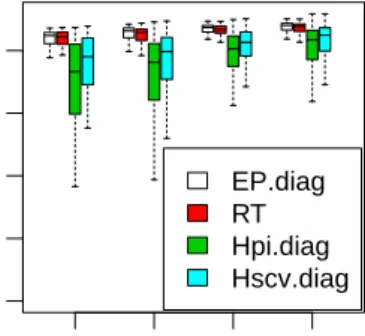
elihood n EP.diag RT Hpi.diag Hscv.diag
Figure 8: Average test log-likelihood on the Earthquake data sets
In order to evaluate the performance of the proposed method in real scenarios, we report a comparative study on its generalization capabilities. In particular, we sampled a subset of size n from the data set and we used it to estimate the density function. We used such an estimate to compute the average log-likelihood of the remaining data; this is a reasonable measure of the generalization capabilities of the procedure, as it provides an estimate of the goodness of the fit to unseen data. We repeated this procedure for
different values ofn and 100 times for each value ofn. The results are shown in Figs. 7 and 8. We selected a full precision in the Unicef data and a diagonal precision for the Earthquake data. In fact, we could have used the estimated Bayes factors to select the most likely covariance structure at each iteration; since the comparing methods do not provide this feature, we preferred to choose one particular structure only and report the corresponding results. In the case of the earthquake data, Hlscv was not converging to any solution
in some cases, and we do not report it in the plot.
The proposed method performs quite well in terms of generalization. Es-pecially in the earthquake data set, the method is significantly better than the plug-in ones. Interestingly, the rule of thumb works quite well too. In the other two data sets, the performance is comparable to the other methods.
In general, considering all the experimentations presented in the last two sections, we see that the performance is at least as good as that of the comparing methods. We remark, however, that the proposed method is not based on the optimization of any sort of performance measure, but simply on the Bayesian principle.
7. Conclusions
We presented an approximate Bayesian approach to the selection of the bandwidth in KDE. The method is based on a cross-validated likelihood, and computes an approximation to the intractable posterior over the band-width. The approximation is carried out by the EP algorithm, which is based on matching the moments with appropriate approximating distributions. In our case we selected the Wishart distribution for the approximations, given its suitability for modeling distributions over positive definite matrices. We demonstrate that the proposed method is competitive in terms of accuracy with existing approaches and we extensively studied the results of the in-ference process. In particular, we showed how it is possible to choose the structure of covariance to use, and how to infer the bandwidth by updating the posterior distribution inferred from a former batch of data. Our approach is closely related to the sampling-based approach of Zhang et al. (2006), but exploits the typical speed of deterministic approximate methods, while still retaining an excellent approximation to the posterior distribution.
On a more general note, it is interesting to notice the similarity between KDE and non-parametric Bayesian approaches to density estimation. In par-ticular, Dirichlet Process Mixture Models (DPMMs) (Ferguson, 1973) have
received considerable attention in the machine learning community as they present a flexible method for clustering and density estimation. In DPMMs, the marginal data density (i.e. having marginalized the latent cluster mem-bership variables) is also represented as a mixture of a (potentially infinite) number of Gaussians. However, unlike KDE, the number of Gaussian com-ponents inferred from a finite sample is in general not equal to the number of data points; also, we are not aware of L2 convergence properties for DP-MMs. In terms of inference, although an EP approach has been proposed for DPMMs (Minka and Ghahramani, 2003), block Gibbs sampling remains the most widely adopted choice within this context.
Appendix A. Special Cases for Expectation Propagation Appendix A.1. Diagonal Precision Matrix
The unnormalized Gamma distribution is defined as ˜
G(λ|a, b) =λa−1exp(−bλ),
and the Gamma distribution
G(λ|a, b) = BG(a, b) ˜G(λ|a, b),
where
BG(a, b) =
ba Γ(a).
We consider a diagonal form for the precision Λ, where diag(Λ) =λ. The
fac-tors for the approximation of the posterior factorize between the covariates, and are defined as
˜ fi(λ) = γi d Y k=1 ˜ G(λk|aik, bik), which gives q(λ) = n Y i=0 γi ! d Y k=1 ˜ G λk n X i=0 aik−n, n X i=0 bik ! .
The true posterior is
p(λ|X)∝
n
Y
i=0
where f0(λ) = Qd
k=1G(λk|a0k, b0k) denotes the prior, and the components
fj(λ) are fj(λ) =p(xj|λ,MX) = 1 n−1 n X r6=j,r=1 N(xj|xr,Λ),
with Λ diagonal and diag(Λ) = λ.
When we remove the j-th component from q(λ), we obtain
q\j(λ) = n Y i6=j,i=0 ˜ fi(λ) = n Y i6=j,i=0 γi ! d Y k=1 ˜ G λk n X i6=j,i=0 aik−n+ 1, n X i6=j,i=0 bik ! . Let’s define: αk = n X i6=j,i=0 aik−n+ 1 + 1 2, βrk = n X i6=j,i=0 bik+ 1 2(xrk−xjk) 2, ψ = n Y i6=j,i=0 γi ! 1 (n−1)(2π)d/2, zr = d Y k=1 BG(αk, βrk)−1. With the definitions above, we see that
fj(λ)q\j(λ) = ψ n X r6=j,r=1 zr d Y k=1 G(λk|αk, βkr)
Now we have to match the moments of
q(Λ|anew, bnew) =γnew d
Y
k=1
BG((ak)new,(bk)new)−1G(λk|(ak)new,(bk)new)
with those of fj(Λ)q\j(λ). The normalization constant is: E0 = Z fj(λ)q\j(λ)dλ=ψ n X r6=j,r=1 zr
For the mean and the variance we notice that the resulting density is a weighted sum of products of Gamma across the covariates
fj(λ)q\j(λ)∝ n X r6=j,r=1 wr d Y k=1 G(λk|αk, βkr),
where the weights are
wr =
zr
Pn
s6=r,s=1zs .
Therefore, the expected value and the variance are
E1k= Efj(λ)q\j(λ)[λk] = n X r6=j,r=1 wr αk βrk , E2k = Efj(λ)q\j(λ)[λ 2 k]−E12k= n X r6=j,r=1 wr " αk (βrk)2 + αk βrk 2# −E12k.
For the updated version qnew(λ) we have
E0 = Z qnew(λ)dλ=γnew d Y k=1 BG((ak)new,(bk)new)−1, E1k = Eqnew(λ)[λk] = (ak)new (bk)new , E2k = varqnew(λ)[λk] = (ak)new ((bk)new)2 .
This allows to compute γnew, (ak)new, and (bk)new
(ak)new = E2 1k vk , (bk)new = E1k vk , γnew =E0 d Y k=1 BG((ak)new,(bk)new).
The updated version of ˜fj(Λ) is the ratio betweenqnew(λ) andq\j(λ), result-ing in ˜ fj′(λ) =γ′ j d Y k=1 ˜ G(λ|a′ jk, b′jk),
with γjk′ = Qnγnew i6=j,i=0γi , a′jk = (ak)new+n− n X i6=j,i=0 aik, b′jk = (bk)new− n X i6=j,i=0 bik.
After the convergence criterion is satisfied, the resulting approximating posterior is q(λ) =γ d Y k=1 ˜ G(λk|ak, bk),
that allows to obtain the approximate model evidence as evidence =γ
d
Y
k=1
BG(ak, bk)−1.
Appendix A.2. Isotropic Precision Matrix
The proposed approximation of the posterior over the precision λ, in the case of a precision matrix Λ =λI is
q(λ) = n Y i=0 ˜ fi(λ),
where the factors in the approximation are defined as ˜ fi(λ) = γiG˜(λ|ai, bi) and therefore q(λ) = n Y i=0 γi ! ˜ G λ n X i=0 ai−n, n X i=0 bi ! .
The true posterior is
p(λ|X)∝
n
Y
i=0
where f0(λ) =G(λ|a0, b0) denotes the prior, and the components fj(λ) are fj(λ) = p(xj|λ,MX) = 1 n−1 n X r6=j,r=1 N(xj|xr, λI).
When we remove the j-th component fromq(λ), we obtain
q\j(λ) = n Y i6=j,i=0 ˜ fi(λ) = n Y i6=j,i=0 γi ! ˜ G λ n X i6=j,i=0 ai−n+ 1, n X i6=j,i=0 bi ! .
Let’s define the following quantities:
α= n X i6=j,i=0 ai−n+ 1 + d 2, βr = n X i6=j,i=0 bi+ 1 2kxr−xjk 2, ψ = n Y i6=j,i=0 γi ! 1 (n−1)(2π)d/2, zr=BG(α, βr)−1. With the definitions above, we see that
fj(λ)q\j(λ) =ψ n
X
r6=j,r=1
zrG(λ|α, βr).
Now we have to match the moments of
q(λ|anew, bnew) =γnewBG(anew, bnew)−1G(λ|anew, bnew)
with those of fj(λ)q\j(λ). The normalization constant offj(λ)q\j(λ) is
E0 = Z fj(λ)q\j(λ)dλ=ψ n X r6=j,r=1 zr
For the mean and the variance, we notice that the resulting density is a weighted sum of Gamma
fj(λ)q\j(λ)∝ n X r6=j,r=1 wrG(λ|α, βr) with weights wr = zr Pn s6=r,s=1zs . Therefore E1 = Efj(λ)q\j(λ)[λ] = n X r6=j,r=1 wr α βr , E2 = Efj(λ)q\j(λ)[λ 2]−E2 1 = n X r6=j,r=1 wr " α (βr)2 + α βr 2# −E12.
For the updated version qnew(λ) we have
E0 =
Z
qnew(λ)dλ=γnewBG(anew, bnew)−1,
E1 = Eqnew(λ)[λ] = anew bnew , E2 = varqnew(λ)[λ] = anew (bnew)2. This allows to compute γnew, anew, and bnew as
anew = E2 1 E2 , bnew = E1 E2
, γnew =E0BG(anew, bnew).
The updated version of ˜fj(λ) is the ratio betweenqnew(λ) andq\j(λ), resulting in ˜ fj′(λ) = γj′G˜(λ|a′j, b′j), where γj′ = Qnγnew i6=j,i=0γi , a′j =anew+n− n X i6=j,i=0 ai,
b′j =bnew−
n
X
i6=j,i=0
bi.
After the convergence criterion is satisfied, the resulting approximating posterior is
q(λ) =γG˜(λ|a, b),
that allows to obtain the approximate model evidence as evidence =γ BG(a, b)−1.
References
Bishop, C. M., 2007. Pattern Recognition and Machine Learning (Informa-tion Science and Statistics), 1st Edi(Informa-tion. Springer.
Bowman, A. W., 1984. An alternative method of cross-validation for the smoothing of density estimates. Biometrika 71 (2), 353–360.
Brewer, M. J., 2000. A Bayesian model for local smoothing in kernel density estimation. Statistics and Computing 10 (4), 299–309.
Calderhead, B., Girolami, M., 2009. Estimating Bayes factors via thermo-dynamic integration and population MCMC. Computational Statistics & Data Analysis 53 (12), 4028–4045.
Cao, R., Cuevas, A., Manteiga, W. G., 1994. A comparative study of sev-eral smoothing methods in density estimation. Computational Statistics & Data Analysis 17 (2), 153–176.
Chiu, S. T., 1991. Bandwidth selection for kernel density estimation. The Annals of Statistics 19 (4), 1883–1905.
de Lima, M. S., Atuncar, G. S., 2011. A Bayesian method to estimate the optimal bandwidth for multivariate kernel estimator. Journal of Nonpara-metric Statistics, 137–148.
Duong, T., Cowling, A., Koch, I., Wand, M. P., 2008. Feature significance for multivariate kernel density estimation. Computational Statistics & Data Analysis 52 (9), 4225–4242.
Duong, T., Hazelton, M. L., 2005. Cross-validation bandwidth matrices for multivariate kernel density estimation. Scandinavian Journal of Statistics Theory and Applications 32 (3), 485–506.
Ferguson, T. S., 1973. A Bayesian analysis of some nonparametric problems. The Annals of Statistics 1 (2), 209–230.
Filippone, M., Masulli, F., Rovetta, S., 2010. Applying the possibilistic c-means algorithm in kernel-induced spaces. IEEE Transactions on Fuzzy Systems 18 (3), 572–584.
Friel, N., Pettitt, A. N., 2008. Marginal likelihood estimation via power posteriors. Journal of the Royal Statistical Society: Series B (Statistical Methodology) 70 (3), 589–607.
Gangopadhyay, A., Cheung, K., 2002. Bayesian approach to the choice of smoothing parameter in kernel density estimation. Journal of Nonpara-metric Statistics 14 (6), 655–664.
Gelman, A., Rubin, D. B., 1992. Inference from iterative simulation using multiple sequences. Statistical Science 7 (4), 457–472.
Hall, P., 1982. Cross-validation in density estimation. Biometrika 69 (2), 383–390.
Hastings, W. K., 1970. Monte Carlo sampling methods using Markov chains and their applications. Biometrika 57 (1), 97–109.
Hazelton, M. L., Turlach, B. A., 2007. Reweighted kernel density estimation. Computational Statistics & Data Analysis 51 (6), 3057–3069.
Jones, M. C., 1991. On correcting for variance inflation in kernel density estimation. Computational Statistics & Data Analysis 11 (1), 3–15. Jones, M. C., Henderson, D. A., 2009. Maximum likelihood kernel density
es-timation: On the potential of convolution sieves. Computational Statistics & Data Analysis 53 (10), 3726–3733.
Jones, M. C., Marron, J. S., Park, B. U., 1991. A simple root n bandwidth selector. The Annals of Statistics 19 (4), 1919–1932.
Jones, M. C., Marron, J. S., Sheather, S. J., 1996. A brief survey of band-width selection for density estimation. Journal of the American Statistical Association 91 (433), 401–407.
Kass, R. E., Carlin, B. P., Gelman, A., Neal, R. M., 1998. Markov chain Monte Carlo in practice: A roundtable discussion. The American Statisti-cian 52 (2), 93–100.
Kass, R. E., Raftery, A. E., 1995. Bayes factors. Journal of the American Statistical Association 90 (430), 773–795.
Kulasekera, K. B., Padgett, W. J., 2006. Bayes bandwidth selection in kernel density estimation with censored data. Journal of Nonparametric Statistics 18 (2), 129–143.
Loader, C. R., 1999. Bandwidth selection: classical or plug-in? The Annals of Statistics 27 (2), 415–438.
Marron, J. S., Wand, M. P., 1992. Exact mean integrated squared error. The Annals of Statistics 20 (2), 712–736.
Metropolis, N., Rosenbluth, A. W., Rosenbluth, M. N., Teller, A. H., Teller, E., 1953. Equation of state calculations by fast computing machines. The Journal of Chemical Physics 21 (6), 1087–1092.
Minka, T. P., 2001. Expectation propagation for approximate Bayesian in-ference. In: Uncertainty in artificial intelligence: proceedings of the sev-enteenth conference (2001), August 2-5, 2001, University of Washington, Seattle, Washington. Morgan Kaufmann, p. 362.
Minka, T. P., Ghahramani, Z., 2003. Expectation propagation for infi-nite mixtures. Tech. rep., NIPS’03 Workshop on Nonparametric Bayesian Methods and Infinite Models, 13, Whistler, BC Canada.
Neal, R. M., 1993. Probabilistic inference using Markov chain Monte Carlo methods. Tech. Rep. CRG-TR-93-1, Dept. of Computer Science, University of Toronto.
Opper, M., Winther, O., 2000. Gaussian processes for classification: Mean-field algorithms. Neural Computation 12 (11), 2655–2684.
R Development Core Team, 2006. R: A Language and Environment for Sta-tistical Computing. R Foundation for StaSta-tistical Computing, Vienna, Aus-tria.
Rinaldo, A., Wasserman, L., 2010. Generalized density clustering. Annals of Statistics 38 (5), 2678–2722.
Sheather, S. J., Jones, M. C., 1991. A reliable data-based bandwidth selec-tion method for kernel density estimaselec-tion. Journal of the Royal Statistical Society. Series B (Methodological) 53 (3), 683–690.
Silverman, B. W., 1986. Density Estimation for Statistics and Data Analysis (Chapman & Hall/CRC Monographs on Statistics & Applied Probability), 1st Edition. Chapman and Hall/CRC.
Skilling, J., 2006. Nested sampling for general Bayesian computation. Bayesian Analysis 1 (4), 833–860.
Terrell, G. R., 1990. The maximal smoothing principle in density estimation. Journal of the American Statistical Association 85 (410), 470–477.
Tran, T. N., Wehrens, R., Buydens, L. M. C., 2006. KNN-kernel density-based clustering for high-dimensional multivariate data. Computational Statistics & Data Analysis 51 (2), 513–525.
van der Laan, M. J., Dudoit, S., Keles, S., 2004. Asymptotic optimality of likelihood-based cross-validation. Statistical Applications in Genetics and Molecular Biology 3 (1).
Wand, M. P., Jones, M. C., 1994. Multivariate plug-in bandwidth selection. Computational Statistics 9, 97–116.
Zhang, X., Brooks, R. D., King, M. L., 2009. A Bayesian approach to band-width selection for multivariate kernel regression with an application to state-price density estimation. Journal of Econometrics 153 (1), 21–32. Zhang, X., King, M. L., Hyndman, R. J., 2006. A Bayesian approach to
band-width selection for multivariate kernel density estimation. Computational Statistics and Data Analysis 50 (11), 3009–3031.
˙Zychaluk, K., Patil, P., 2008. A cross-validation method for data with ties in kernel density estimation. Annals of the Institute of Statistical Mathe-matics 60 (1), 21–44.