Future Realized Return, Firm-Specific Risk and the Implied Expected Return

(1)

1

Future Realized Return, Firm-Specific Risk and the Implied Expected Return

Pengguo Wang1

Xfi Centre for Finance and Investment Exeter University Business School

Exeter EX4 4ST, UK

1_{I thank David Ashton, Mark Clatworthy, Daniela Acker, Alan Gregory, Mike Jones, Stuart McLeay (EAA}

discussant), Peter Pope, Mark Tippett and seminar participants at University of Birmingham, University of Bristol, Warwick University, University of Swansea, Nottingham University (Ningbo), Beijing University, Wuhan University, Fuzhou University and EAA2014 for helpful comments and suggestions. I would like to express my thanks to an anonymous referee as well as the editor Stewart Jones and associate editor David Johnstone for their helpful comments. Finally, I am gratefully acknowledge the financial support of the Economic and Social Research council under award # ES/J023914/1.

(2)

2

Abstract

In this paper, we propose a novel approach to derive a firm-specific measure of expected

return. It builds on recent accounting-based valuation models developed by Clubb (2013) and

Ashton and Wang (2013). The measure is intrinsically linked to commonly used financial

ratios including book-to-market, (forward) earnings yield, dividend-to-price as well as growth

and past returns. The empirical evidence shows that it is significantly positively associated

with future realized stock returns and also significantly correlates with commonly used risk

characteristics in a theoretically predictable manner. The results are likely to be of interest to

practitioners and managers in making capital allocation decisions and to academics in need of

proxies for firms’ discount rates and expected returns.

Keywords: Implied risk premium; Firm risk characteristics; Earnings forecasts JEL: G12, G32, M41

(3)

3

1. Introduction

A growing number of studies in finance and accounting employ the implied cost of equity

capital or the internal rate of return as a proxy for expected stock returns.2 However, the proxy

often fails to reliably predict future stock returns (Pastor et al. (2008)). Moreover, the

cross-sectional relationship between the proxy and firm-specific risk characteristics is inconclusive

(Botosan and Plumlee (2005)).3 In this paper, we develop a novel approach to estimate

expected one-period ahead stock returns by projecting future returns onto a set of accounting

fundamentals and market variables embedded in recent accounting-based valuation models.

We show that our proxy for expected stock returns is significantly positively associated with

future realized stock returns and also significantly correlates with commonly used risk

characteristics in a theoretically predictable manner.

By extending Clubb (2013) and Ashton and Wang (2013), we demonstrate that firm-specific

one-period ahead returns are intrinsically linked to the commonly used financial ratios

including book-to-market, (forward) earnings yield, dividend-to-price, as well as growth and

past returns. Since the linkage is built on the established accounting-based valuation models,

expected one-period ahead return is labeled as the implied expected return (IER). Our

expression identifies firm characteristics that are associated with risky future growth as

explaining the IER. It provides an explanation for why book-to-market (B/P) may be useful for

2_{Pastor et al. (2008) apply the implied cost of equity capital (ICC) approach to test the Intertemporal CAPM,} while Lee et al. (2009) use the ICC to test international asset pricing models. The ICC methodology has been used to examine whether cross-listing reduces foreign firms’ cost of capital and the effectiveness of a country’s legal institutions and securities regulation (Hail and Leuz (2006, 2009)). The ICC approach has also been employed to investigate default risk (Chava and Purnanadam (2009)) and executive pay disparity (Chen et al. (2013)).

3_{The correlations between many expected return proxies and realized returns are often not statistically different} from zero. Some studies find a positive relation between the ICC and market beta (Kaplan and Ruback (1995), Gode and Mohanram (2003)), and some find a negative relation (Hou et al. (2012) ), while others find this relation to be mostly insignificant (Gebhardt et al. (2001), Lee et al. (2009)).

(4)

4

explaining expected stock returns.4 It shows that neither should book-to-market be viewed as

a risk factor, nor does market-to-book (P/B) itself represent growth as commonly interpreted.

However, B/P interacts with the growth of future investments, so investors may rationally take

it into account in pricing equity shares. It also shows that the IER is associated with forward

earnings yield that is related to uncertainty about future earnings. This is consistent with

Penman and Zhu (2014) and Penman (2016), who express expected returns in terms of

expectations of earnings and earnings growth.5_{Furthermore, it shows that accounting}

conservatism can cause time-serial correlation in stock returns.

The coefficients of the financial ratios in the IER expression are functions of five valuation

parameters including expected long term growth of the NPV of future investments and long

term cost of capital based on currently available information. Following Ashton and Wang

(2013), we use one-year ahead forecasts of earnings and estimate simultaneously the five

valuation parameters according to a long-standing industry practice of using benchmark

industry averages in the valuation of an individual firm (Damodaran (2002), Liu et al. (2002),

Penman (2010)).6

The existing literature evaluates the usefulness of a proxy for expected stock return mainly by

testing whether it can predict realized returns. We show that the implied expected return is

significantly positively associated with future realized stock returns for a sample of I/B/E/S

U.S. firms over the period 1980-2011. The measure remains significantly positively related to

4_{Liew and Vassalou (2000) find that book-to-market and size portfolios are related to future growth in the real} economy. Book-to-market has been explained as growth options (Berk et al. (1999)) and investment and asset growth (Cooper et al. (2008)). Vassalou (2003) argues that news related to future GDP growth can explain the cross-section of equity returns as well as the Fama-French model can.

5_{Penman and Zhu (2014) document that variables that forecasts earnings and earnings growth also forecasts} expected returns. Penman et al. (2014) also identify forward earnings yield as an omitted factor from a

characteristic model. However, in contrast to our model, the expression in Penman et al. is a tautology (Penman (2016, p.110)). The return decomposition developed by Easton and Monahan (2005) is also based on two tautologies (Easton and Monahan (2016 p.45)).

6_{The main advantages of Ashton and Wang (2013) method are that it does not explicitly assume dividend}

payout policy and requires only one-year-ahead forecasts of earnings. However, it only allows one to estimate the average implied cost of capital and growth rate for a given portfolio of firms.

(5)

5

future realized stock returns, even after controlling for commonly used risk proxies (the CAPM

beta, size and leverage) and cash flow and discount rate news (Campbell (1991), Vuolteenaho

(2002)), as well as term spread and default spread (Fama and French (1989)). We also

document the IER’s out-of-sample predictive ability with respect to future stock returns by

sorting firms into quintiles of IER distribution each year. For each portfolio, the mean

buy-and-hold returns for the next 12- and 60-month are calculated. We find that the IER measure

exhibits a monotonic relation with future realized returns. Hedge return, the difference in the

cumulative 60-month realized returns between the top and bottom quintiles of the IER, is equal

to 46.6%. Prior literature that assesses the validity or reliability of firm-specific estimates of

expected return has also been motivated on correlations with commonly used risk proxies. In

this respect, our measure is associated with conventional risk characteristics in a theoretically

predictable manner. Specifically, it shows a significant positive relation between expected risk

premium and market beta, leverage, default spread, and negative association between implied

risk premium and firm size.

The rest of the paper is organized as follows. Section 2 introduces an accounting-based

valuation model and discusses the intrinsic relationship between the implied one-period ahead

return and various fundamental characteristics of a firm. Section 3 describes the sample and

empirical implementation in estimating of the implied expected return. Section 4 provides the

estimation results and assesses the validity of the estimates. Section 5 concludes.

2. The Implied One-Period Ahead Return and Firm Characteristics

Assuming information dynamics on abnormal earnings, book values, dividends, the

no-arbitrage condition and clean surplus accounting, Clubb (2013) extends the Ohlson (1995)

(6)

6

dividend ( d_t ), and abnormal earnings ( x_ta ) as7:

P

_t

= +

(1

β

₁

)

b

_t

+

β

₁

d

_t

+

β

₂

x

_ta , where

1

( 1)

a

t t t

x = −x R− b₋ , x is earnings, R is one plus the long term average cost of equity capital _t

based on time t information. While this expression demonstrates that dividends displace both

book value and market value on a dollar-for-dollar basis, it does not consider explicitly the

present value of all future investments. In related research, Ashton and Wang (2013) introduce

a growth variable that describes the net present value of all future investments (

ϑ

_t). Naturally, we merge these two models as below:

1 1 2 (1 ) a t t t t t P = +

β

b +

β

d +

β

x +

ϑ

(1) 1 (1 ) ( 1 ) 1 t g t Pt dt Pt xt t

ϑ

+ = +

ϑ λ

+ + − − − +

ε

+ (2)

where g (< R-1) is the long term average growth rate of the net present value of future ex ante

investments based on time t information. The second term on the right hand side of equation

(2) adjusts for the potential impact of accounting conservatism since conservatism in reporting

may influence beliefs about future profitability when the expectation of growth is formed.8

Here λ_{is labeled as a conservatism parameter and conservatism is measured by the difference}

between economic earnings,

(

P

_t

−

P

_t₋₁

+

d

_t

)

, and accounting earnings. Valuation multiples satisfy

β

₁≥(R−1)

β

₂ >0.9

ε

_t₊₁ is an error term with mean zero.

7_{This model is also consistent with Collins et al. (1999) and Pope and Wang (2005).}

8_{Claus and Thomas (2001) argue that expected growth is affected by both the expectation of future economic}

rents and the conservative nature of accounting. Conservative accounting implies ‘something about the future payoff’ (Johnstone (2016, p.2)).

9_{Note that equation (1) can be rewritten as}

1 2 1 2 2

[1 ( 1) ] [ ( 1) ]

t t t t t

P = + −β R− β b + β − R− β d +Rβ x +ϑ . Equity

value is expected to increase in the firm’s (abnormal) earnings in general (β₂ >0). For a majority of firms book values are understated under conservative accounting. For example, physical assets are recorded at historical costs; inflation and associated asset holding gains are ignored; R&D is sometimes viewed as an expense rather than an investment; and many intangible assets are not recognized. We would expect the coefficient of book value is greater than 1, or β₁≥(R−1)β₂>0.

(7)

7

Assuming the clean surplus accounting (i.e.,

b

_t₊₁

+

d

_t₊₁

=

x

_t₊₁

+

b

_t), equations (1) and (2) imply the one-period ahead total return:

1 1 1 1 1 2 1 2 [1 ( 1) ] [1 ] t t t t t t t t t P d b x R P P P P

ϑ

β

β β

+ + + _{= + −} ₋ _{+ + +} + ₊ + _. ₍₃₎

All proofs can be found in the appendix. The positive association between book-to-market ratio

(B/P) and equity return becomes apparent when we control for forward earnings yield and ratio

of one-period ahead NPV of future investments to price. When regressing expected return on

book-to-market, and either reasonable proxies for t[ t 1]

t E P

ϑ

₊ and t[ t 1] t E e P

+ _{, or both forward ratios}

are missing, one would observe that B/P is positively related to expected returns. This is

consistent with findings in Fama and French (1988, 1992, 1993, 2006) and others.

In parallel with the standard dividend growth model, equation (3) can be written in terms of

growth, dividend yield, abnormal growth in book value and abnormal growth in forward

earnings as: 1 1 1 1 2 1 1 1 1 2 (1 ) 1 (1 ) (1 ( 1) ) (1 ) ( ) (1 ) [ ] . t t t t t t t t t t t t t t t t t t P d d b g b g g R P P P x g x P d P x P P P

β

ε

β β

λ

+ + − + − + + _{= + + +} _{+ + −} ₋ − + − + + − − + + + + + (4)

It is clear that equity returns and growth are interlinked (Penman (2016)). In particular, if we

set

β β

₁ = ₂ =0, and

λ

=

0

, equation (4) reduces to

1 1 1 1 1 t t t t t t t t t P d x b g g P P P P

ε

+ + + _{− = +} + ₋ ₊ + _. ₍₅₎

Equation (5) shows that B/P is negatively related to the one-period ahead return and B/P

amplifies the growth after controlling for growth and forward earnings yield.10 This is in

(8)

8

contrast to a large body of empirical asset pricing literature. If there is no growth (g=0), then

B/P should not have explanatory power to expected returns. This parsimonious model suggests

that neither should book-to-market be viewed as a risk factor, nor does market-to-book (P/B)

itself represent growth as commonly interpreted. Although the forward earnings yield has long

been used in equity valuation by financial analysts, it appears until recently that not enough

attention has been paid to forward earnings in the empirical asset pricing literature (Fame and

French (2006), Lyle et al. (2013), Penman (2016)).

It is also interesting to note that equation (4) provides an alternative explanation as to why

current returns may be associated with future returns. It shows that accounting conservatism

can cause time-serial correlation in stock returns. Accounting conservatism understates ‘true’

current incomes, or only recognizes a portion of economic earnings. The unrecognized portion

will be recognized at a later stage and may be reflected in future returns. 11 The conservative

nature of reporting may influence investors’ beliefs about future profitability when

expectations of growth and future earnings are formed.

Since dividends in equation (4) are dividends net of new capital contributions, for our purpose

we replace dividends by lagged book value via the clean surplus accounting,

d

_t

= +

x

_t

b

_t₋₁

−

b

_t. It follows from (4) that12

1 1 1 1 2 1 2 1 2 1 1 1 1 2 (1 )[1 ( ( 1) ) ( ) ] (1 ( 1) ) ( ) (1 ) [ ] . t t t t t t t t t t t t t t t t t t t t P d b b x b g R R P P P P P x P d P x P P P

β

β β

β

ε

β β

λ

+ + − + − + + _{= +} _{− −} ₋ ₋ ₋ ₊ _{+ + −} ₋ + − − + + + + + (6) the B/P increases for a fixed earnings yield.

11_{If an asset is over depreciated, for instance, then it will be under depreciated at some future date as there exists} a reversing process.

12_{This expression shows explicitly what ‘added accounting variables’ in the return model in Penman and Zhu}

(9)

9

Therefore, the implied one-period ahead equity returns are intrinsically linked to the commonly

used financial ratios including book-to-market and (forward) earnings yield, as well as growth

and past returns.13

In order to estimate the expected one-period ahead return based on equation (6), we need to

estimate valuation parameters (

β β λ

₁, ₂, , ,R g ), for given firm-specific information or accounting ratios and forecasted one-period ahead earnings. While an individual firm’s

valuation parameters in equations (1) and (2) may be estimated according to a long-standing

industry practice of using benchmark industry averages (Damodaran (2002), Liu et al. (2002),

Penman (2010)), it is still a challenge to estimate simultaneously R and g. The terminal growth

rate used to truncate infinite future cash flows in a valuation model is often assumed by

researchers.14 Fortunately, recent advances in the implied cost of capital literature provide us

with techniques to estimate simultaneously all valuation parameters including R and g for a

given portfolio of firms.15 Therefore, we do not have to assume the same growth rate for all

firms as in the existing implied cost of capital literature. Instead, we differentiate growth rates

across portfolios (industries) to distinguish different growth opportunities and different risk

(Penman (2016)). The approach developed in Ashton and Wang (2013) among others has some

other notable advantages in terms of information requirements since it does not explicitly

assume dividend payout policy and requires only one-period ahead forecasts of earnings.16

13_{This is also consistent with Lyle et al. (2013) and Callen (2016), who show that expected return can be written} in terms of book-to-price, (forward) earnings-to-price and dividend-to-price when abnormal earnings dynamic follows a mean-reverting process. Recently, Christodoulou et al. (2016) also show that the ICC can be estimated using only reported accounting information and without reference to stock price.

14_{For example, Claus and Thomas (2001) assume that residual incomes grow at the same rate (i.e. an estimate} of the expected inflation rate) across all firms. Dargenidou et al.(2006) also use the government bond yield (the risk free rate ) as a proxy for long term growth.

15_{Penman argues that ‘the joint estimation of ER (the implied cost of capital) and g in Easton et al. (2002) as if} they were independent inputs to a valuation is suspect if growth is risk’(Penman (2016, p.119)). Equation (11) in the appendix shows that estimating the implied cost of capital and growth rate simultaneously does not mean that they are independent inputs. One can first estimate g, then the implied cost of capital as a function of g and other parameters.

16_{Dividend payout policy is usually supposed over a forecast period, and multiperiod forecasts of earnings or} price targets are normally required in the existing literature. For instance, Gebhardt et al. (2001) rely on up to

(10)

10

The key step to the Ashton and Wang approach is to express the expected one-period ahead

earnings in terms of accounting fundamentals and stock prices. In our model setup, equations

(1) and (2), together with the no-arbitrage condition and clean surplus accounting imply that

the expected one-period ahead earnings can be written as:

1 2 1 2 1 1 2 1 2 1 2 1 2 1 1 1 2 1 2 (1 )( ) ( 1) (1 ) [ ] (1 ) (1 ) (1 ) (1 )( ( 1) ) . (1 ) (1 ) t t t t t t t g g R R g E x P x b g R b P

β β

β

β λ

λ

β β

β

λ

β β

+ − − + + − + − + − + − = + + + + + + + + + − − − + + + + + + (7)

Given a proxy of expected earnings, cross-sectional regressions will give the estimates for

coefficients attached to price, earnings and book value in equation (7). From the corresponding

five coefficients, we can estimate simultaneously the implied cost of equity capital (R-1),

growth rate (g) and valuation parameters,

β β

₁, ₂ and

λ

, for a given portfolio of firms, or an industry.

3. Describing Sample and Empirical Implementation

3.1 Sample Description

The sample includes all NYSE, Amex and Nasdaq listed securities. Data are extracted from the

CRSP monthly returns file from January 1975 to June 2011, and the Compustat industrial

annual file from 1978 to 2010 and forecasts of earnings from the Institutional Brokers Estimate

System (I/B/E/S) between 1979 and 2010. The adjusted number of shares outstanding and

adjusted price at the end of the fiscal year, and adjusted price of equity three months after the

fiscal year-end are collected from CRSP.17 Stock price three months after the fiscal year-end is

three years of earnings forecasts and assume that firms have a 100% dividend payout ratio beyond the forecast horizon. Claus and Thomas (2001) assume that 50% of earnings are retained each period. Easton et al. (2002) are based on up to four years of earnings forecasts and assume that the expected dividends in the subsequent four years are equal to the current dividends paid.

(11)

11

used to ensure that information about the prior year financials has been incorporated in the

analysts’ forecasts of earnings. Accordingly, 12-month buy-and-hold returns for each firm from

April to March each year are calculated.18 This is also consistent with the fact that a majority

of firms have fiscal year end in December.19 Relevant accounting data are collected from

Compustat. Firms with negative book values (CEQ) are deleted. Earnings are measured as net

income before extraordinary items (IB). The median consensus forecasts of earnings per share

at the first month after the corresponding I/B/E/S-reported prior-year earnings announcements

are used. All total variables used in the estimation are divided by the adjusted number of shares

outstanding to reduce heteroskedasticity and increase comparability across time. Size is

measured as the logarithm of a firm’s market capitalization, leverage as the total debt divided

by the firm’s market capitalization as of 3-months after the fiscal year end. Total debt is the

sum of long-term debt (DLTT) and short-term debt (DLC). Market beta is estimated via the

market model using the value weighted NYSE/Amex market index return using at least 18 and

up to 60 months of lagged monthly returns. The standard deviations of monthly returns are also

computed using at least 18 months of data over the prior 60 months as a measure of total risk.

In constructing the data set in this analysis, 1% at the top and bottom of book value, earnings,

stock price, number of shares outstanding, and analysts’ consensus forecasts of earnings are

deleted to avoid the influence of extreme observations.

Table 1, Panel A presents the descriptive statistics of the sample firms and analysts’ consensus

forecasts of earnings. We observe that the median of analysts’ forecasts is about 28% higher

calculate the adjusted number of shares outstanding and the adjusted price.

18_{This is in contrast with returns calculated from July to June in Fama and French (1992, 1993, 1995) and} others. Company financials become public information much more quickly compared with two decades ago due to technological advances. In addition, companies are now required by law to publish their accounts in 2-3 months after their fiscal year-end.

(12)

12

than that of actual reported earnings,reflecting the over-optimism of analysts’ forecasts. While

the mean (median) book-to-market is about 0.84 (0.56), the mean of earnings-to-price and the

mean of one-year ahead forward earnings-to-price are 4.8% and 6.7% respectively.

Table 1, Panel B shows the annual cross-sectional correlations for 60,170 observations over

the 31 year period from 1980 to 2010. The upper (lower) right triangle of the matrix presents

Spearman (Pearson) correlations. These correlations show that contemporary price and current

earnings are the variables with the largest correlation coefficients with forecasts of earnings.

3.2 Empirical Implementation

Based on equation (7), the analysis needs only one-year ahead expected earnings and other

contemporary variables. We use one-year ahead analysts’ forecasts of earnings as a proxy of

expected earnings. Given the one-year ahead forecasts of earnings (x_t₊₁) for all the firms within a given portfolio or grouping of firms, we can run the following cross-sectional regressions for

all firms within the portfolio in each year:

1 1 2 3 4 1 5 1 , 1

t t t t t t x t

x₊ =

δ

P +

δ

x +

δ

b +

δ

b₋ +

δ

P₋ +

ε

₊ , (8)

where

ε

e t,+1 is an error term. Therefore the sample long term average growth rate (g), cost of

capital (R), valuation multiples (

β

₁ and

β

₂) and conservatism parameter (

λ

) can all be written in terms of regression coefficients

δ

₁-

δ

₅ applicable to firms within that portfolio as in equations (10)-(12) in the Appendix.

Consistent with industry practice, we use the sample average growth rate, cost of capital and

(13)

13

the firm-specific one-period ahead return.20 Therefore, the firm-specific implied expected

one-period return t[ t 1 t 1 t] t t E P d P IER P + + + −

≡ at time t can be estimated from equation (6) as

1 1 1, 2, 1, 2, 1, 2, 1 1 1, 2, [ ] (1 )[1 ( ( 1) ) ( ) ] (1 ) ( ) (1 ( 1) ) [ ] 1, t t t t t it it it it it it it t it t t t t t t t t t it it it it t t b b x E x IER g R P P P P b P b P b R P P

β

λ

− + − − = + − − − − − + + + + − − − + + − − + − (9)

where Rit,g_it,

α α

_1,_it, _2,_it and

λ

_{i t}_, are long term average cost of capital, growth rate, valuation multiples and conservatism parameter respectively for firms in industry i and year t.

In summary, the analysis has two steps. The first step is to estimate the sample average of cost

of capital, growth rate and valuation multiples based on equations (8), and (10)-(12) on an

industry-year basis. The second step is to compute the firm-specific expected one-year ahead

return based on equation (9). In the following analysis, the 10-year US government bond yield

is subtracted from the IER to compute the implied risk premium. This implied risk premium is

the measure of the expected risk premium (ERP) that is used in the following regression tests.

To examine the (incremental) explanatory power of the implied expected return (IER) on future

realized returns, the relationship between year ahead excess realized stock returns (i.e.

one-year ahead realized returns subtracted by the 10-one-year US government bond yield, XRET1) on

the ERP and other control variables is tested. These control variables include the unexpected

return due to cash flow news, discount rate news and conventional risk characteristics: the

CAPM beta, book-to-market, firm size, leverage, term spread and default spread. A positive

correlation between the ERP and XRET1 provides support for the validity of the IER. A valid

20_{For the purpose of this paper, we estimate the unknown g at the industry-year level and plug it into the model} with firm-specific variables to obtain the firm-specific implied cost of capital. One could well have used a constant implied cost of capital and other coefficients at the industry-year level and estimated a firm-specific g if one’s objective is to estimate firm-specific growth.

(14)

14

proxy of expected return should also be consistent with established asset pricing theory (for

example, Lintner (1965), Sharpe (1964), Modigliani and Miller (1958)). Although the true risk

factors that determine expected returns are unknownor they may not be reliably estimated, as

a first order approximation we can examine the relationship between the expected risk premium

(ERP) and a few well-known risk proxies, such as market beta, leverage, default risk, and the

market value of equity (size).

4. Empirical Results

4.1 Average cost of capital, growth rate and valuation multiples for the industry-year portfolios

We first divide the full sample into 5 industries using the classification from Ken French’s

website. To increase the observations for each of the 150 portfolios in an industry-year analysis,

a two-year rolling window for 30-year over 1980-2009 is used.21 To reduce nonstationarity and

minimize the effects of endogeneity, both sides of equation (8) are deflated by the price three

months after the fiscal year-end to provide contemporaneity with the fiscal year-end reporting

of book values and earnings. The analysts’ forecasts of one-year ahead earnings per share are

used as the dependent variable.

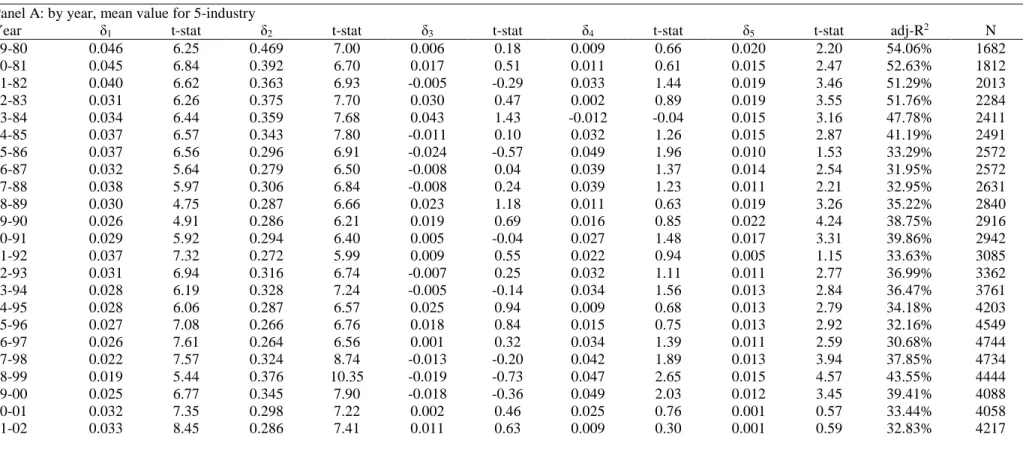
Table 2 reports the parameter estimates in the regression for each of 150 industry-year

portfolios. Panel A shows the average of estimates for all 5-industries on a year-by-year basis.

21_{For example, for year 1980, forecasts of earnings for 1980 and 1981 and accounting data for 1979 and 1980} are used. If industry classification is per Fama-French (1997), it needs more years rolling window to have sufficient observations for firms in some of the 48-industry each year. Consequently, the number of portfolios will increase to 48×30 = 1440.

(15)

15

The sample size varies over the 30 years from a low of 1,682 firms in 1980 to a high of 4859

firms in 2006 over a two-year window. The average number of annual observations is 3,545.

All of the

δ

₁s and

δ

₂s are positive as predicted. We observe that

δ

₁ and

δ

₅ are highly significant with regard to explaining one-year ahead earnings, confirming that prices lead

earnings after controlling for current earnings and book values. We also note that current

earnings (

δ

2) are an important predictor of future earnings. Neither the coefficient of current

book value (

δ

₃) nor the coefficient of lagged book value (

δ

₄) is statistically significant.22 Panel B shows the average of estimates for 30 years on an industry-by-industry basis. The results are

consistent with Panel A. They confirm that prices lead earnings and that earnings are highly

persistent. On average, five variables: current earnings, current and lagged prices, and current

and lagged book values, together explain 38.6% of one-year ahead of analysts’ forecasts of

earnings.

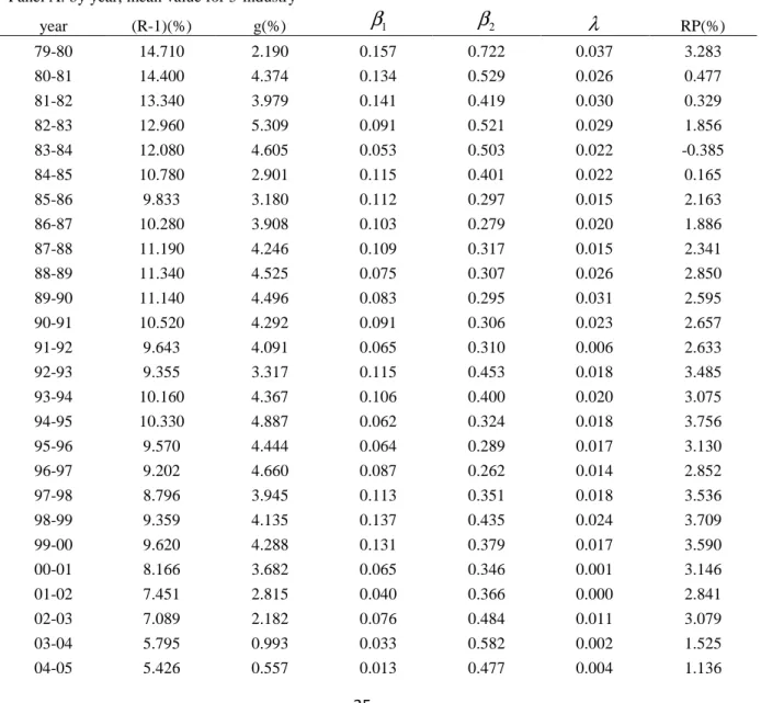
Table 3 details the estimates of long term average cost of capital, growth rates, valuation

multiples, accounting conservatism parameter, and risk premia for the 150 industry-year

portfolios. Similar to Table 2, results on a year-by-year basis (Panel A) and on an

industry-by-industry basis (Panel B) are reported. We observe that the annual mean cost of capital is 9.6%

and the mean risk premium is 2.32% over 1980-2009. Risk premium is based on ten-year U.S.

government bond yields as a proxy for the risk-free rate. Our estimate of the annual mean

growth rate is 3.34%. We also note a downward trend in the cost of capital, with the average

falling from 12% between 1980-1990 to 9.66% between 1991-2000, and finally to 6.48%

between 2001-2009. While the average long-run growth is 3.95% between 1980-2003, the

annual growth rate is not statistically different from zero after 2004. However, as shown in

(16)

16

Figure 1, the risk premium shows an upward trend between 2004-2009, reflecting the fact that

the risk-free rate decreases at a greater rate than the mean IER. This coincides with the recent

financial and credit crisis, and investors demanding a higher risk premium. As expected, all

valuation weight on book value (1+

β

1) is greater than 1 over the 30-year period. All valuation

weights on earnings (

β

₂) are greater than zero and statistically significant at the 1% level. The conservatism parameters (

λ

) is always positive, with a mean value of 0.017. The Fama-MacBeth t-statistics for all five valuation parameters are statistically significant at the 1% level.

Figure 1 illustrates the trend in cost of capital, the risk premium and long-run growth. Results

on an industry-by-industry basis shown in Panel B are similar.

4.2 Firm-specific IER and its relation with realized returns and risk proxies

Applying the parameters estimated in the above analysis to each firm in the 150 industry-year

portfolios, to equation (9) delivers a firm-specific measure of the implied expected one-period

ahead return (IER). Following prior literature (e.g., Campbell, 1991; Vuolteenaho, 2002), when

examining the relationship between the IER and realized future stock returns, we consider cash

flow news (CFN) and discount rate news (DRN). CFN equals actual earnings per share for year

t+1 less analysts’ forecasts of one-year ahead earnings per share or ‘earnings surprise’, scaled

by stock price at time t. Vuolteenaho (2002) suggests that time t discount rate news proxy is a

function of the time t+1 change in the implied expected returns and discount rate news may

not affect all companies equally. Hence, consistent with Easton and Monahan (2005, 2016),

time t discount rate news (DRN), is proxied by (IER_{j t}_, −IER_{j t}_,₋₁) for firm j in the analysis.23

23_{Note Botosan et al. (2011) argue that DRN is an economy-wide discount rate news proxy. In their analysis,} DRN is measured by the one-year ahead change in the yields of the five-year treasury constant maturity as of the month the expected return estimates. If we use their measure, DRN becomes less significant, while the main results are similar.

(17)

17

Following Fama and French (1989) and others, term spread and default spread are also

considered. Term Spread is calculated as the difference between 10-Year US Treasury constant

maturity rate and the 3-month US T-Bill yields. Default Spread is calculated as the difference

between Moody's Seasoned Baa and Aaa Corporate Bond yields. Data on corporate bonds and

US T-Bills/Bonds are obtained from the FRED database of the Federal Reserve Bank of St.

Louis. Further, it may be reasonable to delete firm-year observations with the implied expected

one-year ahead return less than the risk-free rate if the IER is qualified as a proxy for the

expected return (Easton (2009)).24 In the following analysis of the characteristics of expected

return such firm-year observations are eliminated.25 Our interest is in the association between

excess one-year ahead realized returns (XRET1) and excess implied expected risk premium

(ERP).

Table 4 Panel A provides descriptive statistics pertaining to XRET1, ERP, and other risk

proxies. Mean and median estimates of the expected risk premium are 4.7% and 3.5%

respectively.26 While the median XRET1, 3.6% falls within the range of the expected risk

premium, its standard deviation of 60.2% greatly exceeds the standard deviation of ERP. Panel

A also provides descriptive statistics for proxies of cash flow news, discount rate news, term

spread and default spread. CFN has a mean value of -0.044, which is statistically significantly

24_{There are about 24% of firm-year observations with the IER less than the risk-free rate. This includes the} IERs declined between 2001-2009. Note that 31% of the firm-years in the Easton and Monahan (2005) sample (from 1981 to1998) have values of implied cost of equity capital below the risk-free rate. This suggests that the IER is a downward biased measure of expected return. The main results are similar when we drop firm-year observations with the IER less than zero instead of the risk-free rate. Further investigation shows that firms with IER<0 have smaller market capitalization than firms in the full sample (with median 230 vs. 335), smaller (negative) forward (forecasted) earnings yield (with median -1.3% vs. 6.8%) and much higher beta (with median 1.36 vs. 1.04). The averages of B/P are 0.84 and 3.03 respectively for the full sample and firms with IER<0. 25_{The ICC literature also often further restricts the ICC less than 1. As a consequence, the ICCs usually show} the low volatilities and high Sharpe ratios. This is also a limitation of the IER as a proxy of expected return. 26_{If we keep firm-year observations with the IER less than the risk-free rate but greater than 0, then mean and} median estimates of the ERP are 3.46% and 2.75% respectively. Note that the number of observations for XRET1 is slightly smaller than that of IERs since 12 consecutive monthly returns are required to calculate the annual return of a firm.

(18)

18

negative at the 1% level, suggesting optimism in analysts’ earnings forecasts. The mean of

DRN is -0.012 also significantly negative, indicating an average annual decline in the IER over

the sample period. The means of term spread and default spread are 1.685 and 1.095

respectively. The statistics also describe a sample where average market risk is comparable

with that of the market portfolio with a mean (median) beta of 1.058 (0.984) and a mean

(median) debt-to-equity ratio of 69.9% (26%).

Table 4 Panel B presents pair-wise correlations among a set of variables applied in the

regression analysis. It shows that the proxy of expected risk premium ERP correlates positively

with XRET1 with

ρ

= 0.139. As expected, the correlation between XRET1 and CFN is positive (

ρ

=0.194), and that between XRET1 and DRN is negative (

ρ

=-0.159). These correlations are significant at the 1% level, suggesting cash flow news and discount rate news play an important

role in explaining realized returns. Consistent with prior literature, XRET1 is positively related

to leverage and beta, and is negatively related to the size (Fame and French (1992, 1993, 1995)).

Unexpected return, the difference between XRET1 and ERP, also correlates positively with

cash flow news, beta, leverage, term spread and default spread, and negatively with discount

rate news and firm size in a theoretically predictable manner.

Table 4 Panel C documents IER’s out-of-sample predictive ability with respect to future stock

returns by sorting firms into quintiles of implied expected return distribution at the end of

March of each year. For each portfolio, the mean buy-and-hold return for the next 12 months

is calculated. Hedge returns as the difference in returns between the top (Q5) and bottom (Q1)

quintiles of IERs are also calculated. It shows that the IER exhibits a monotonic relation with

future realized returns. The difference in realized returns over 12-months between the top and

bottom quintiles of IER, Q5-Q1, is equal to 8.7%. If the hedge returns represent the expected

(19)

19

shows that the average realized return spreads between quintiles 5 and 1 is 46.6% for 60-month

buy-and-hold returns.

Next, we examine the excess return predictive ability of expected risk premium, ERP, at the

firm level. We also investigate the cross-sectional relation between a set of conventional risk

characteristics and ex post realized return. All regressions are based on a pooled sample, with

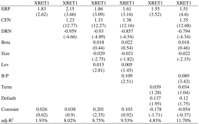
year fixed effects and standard errors clustered by firm and year as in Petersen (2009).27 Table

5 reports coefficients and their t-statistics (in brackets) for these regressions.

Notably, no matter what risk proxies we control for, the implied risk premium has significant

explanatory power to excess one-year ahead realized returns. Both CFN and DRN have

significant incremental roles in explaining future realized returns. Specifically, the result of

univariate regression of excess realized returns on expected risk premium in Table 5 column 2

shows that ERP is positively related to XRET1 with a coefficient of 1.83, which is not

statistically different from 1.28 When we include our proxies for cash flow news and discount

rate news in the regression, it shows a strong positive relation between excess realized returns

and cash flow news and a strong negative relation between excess realized returns and discount

rate news. Adjusted R-squareds increase from 1.93% to 8.02%. When we include term spread

and default spread, the result is similar. The adjusted R-squareds increase from 1.93% to 8.94%.

This result is consistent with our expectation and with results documented in Voulteenaho

(2002) and Botosan et al. (2011). While XRET1 being positively related to beta and leverage,

and negatively related to firm size accords with expectations, neither market beta nor leverage

is significantly related to excess future realized returns if book-to-market is included in the

27_{Fama-MacBeth regressions show more significant results in statistical sense.}

28_{The regression coefficient of the difference between XRET1 and ERP on expected risk premium is 0.83 with}

(20)

20

regression. When including book-to-market in the analysis, both term spread and default spread

have the correct signs but are not statistically significant at the 5% level. The coefficient of

book-to-market itself is positive and highly significant.

Given firm characteristics including growth of future investments, book-to-market,

earnings-to-price, dividends-to-price and past returns are the main inputs in the estimation of the IER,

we only examine the relationship between expected risk premium (ERP) and the CAPM beta,

size, leverage, total risk, term spread and default spread to avoid drawing potential spurious

inferences (Botosan and Plumlee (2005), Easton and Monahan (2016)).29 Based on prior

empirical studies on the cross sectional determinants of returns, we expect the expected return

to be positively associated with beta, leverage, standard deviation of annual return and risk

spreads, and to be negatively associated with firm size.

Table 6 shows that the results of univariate and multivariate regressions of the expected risk

premium on market beta, firm size and leverage are all in the theoretically predicted directions.

Specifically, the expected risk premium is significantly positively related to beta and leverage,

but negatively related to firm size. However, when we control for total risk, there is an

insignificant negative relation between the implied risk premium and beta. The total risk itself

is strongly positively related to EPR, reflecting a property that the I/B/E/S analysts’ forecasts

taking into account more total risk than the firm’s systematic risk.30 In addition, the coefficient

of beta is very stable in magnitude whether we use univariate or multivariate regressions if

excluding total risk. When we include term spread and default spread into the regressions, we

29_{Botosan and Plumlee (2005) argue that spurious effects are likely for most (perhaps all) implied cost of} capital estimates by including book-to-market and earnings yield. It is evident that the adjusted R-squareds are nearly 59% when earnings yield and forward earnings yield are included in our regression analysis.

30_{Hail and Leuz (2006) also suggest that the implied cost of capital seems to be more closely related to stock} return volatility than to beta.

(21)

21

find that default spread is statistically significantly related to the implied risk premium.

However, term spread shows a negative relation though it is not statistically significant.

4.3 Robustness test

Although using benchmark industry averages in the valuation of an individual firm is a

long-standing industry practice, grouping firms based on industry classification is known to be

difficult to ensure homogeneity of firms. Further sorting based on firms’ characteristics is a

natural extension.31 Since the size of different firms within an industry can be significantly

different and size is one of the most important characteristics of a firm, we further group

firms according to their size quintiles in each industry-year portfolio to infer the firm-specific

IER.32 We sort size into 5-quintiles for each of the 150 industry-year portfolios. To increase

the observations for each of the 750 portfolios in an industry-year-size analysis, a five-year

rolling window for 30-year over 1980-2009 is used.

We repeat the analysis above to estimate the average growth rate, cost of capital, valuation

multiples and conservatism parameter for each industry-year-size portfolio, g_ijt,Rijt,

β

_1,_ijt,

β

_2,_ijt

and

λ

ijt, via equation (8), where i=1-5 and j=1-5 represent industry and size respectively. A

modified equation (9) then gives firm-specific proxy of expected returns at year t:

1 1 1, 2, 1, 2, 1, 2, 1 1 1, 2, [ ] (1 )[1 ( ( 1) ) ( ) ] (1 ) ( ) (1 ( 1) ) [ ] 1, t t t t t ijt

ijt ijt ijt ijt ijt ijt t ijt

t t t t

t t t t t ijt

ijt ijt ijt

t t b b x E x IER g R P P P P b P b P b R P P

β

λ

− + − − = + − − − − − + + + + − − − + + − − + −

31_{In addition, analysts’ forecast errors are believed to weaken the association between the implied cost of} capital and realized returns (Hughes et al. (2008)). To mitigate the effect of analysts’ bias, we also adjust the consensus forecasts for predictable errors. The main results, not reported here, are improved only slightly. 32_{Firms in the industry-year portfolios are also further sorted based on firms’ book-to-market ratio or their past} realized returns instead of size. The results are similar. We do not report the detailed results of these tests, but they are available on request.

(22)

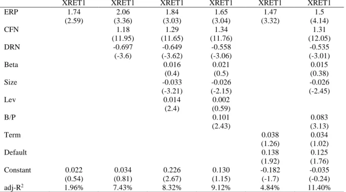
22

The result of univariate regression of excess realized returns (XRET1) on expected risk

premium (ERP) in Table 7 column 2 shows that ERP is positively related to XRET1 with

coefficient of 1.74, which is not statistically different from 1. The adjusted R-squared is similar

to the IER based on the industry-year portfolios. The results of multivariate regressions are also

similar to those when we use the industry-year portfolios. When we include the proxies for

cash flow and discount rate news in the regression, we find the slope increases to 2.06 and CFN

and DRN have significant incremental explanatory power. The adjusted R-squared increases

from 1.96% to 7.43%. While XRET1 is positively related to beta and negatively related to firm

size accord with expectations, only size but not beta is statistically significant when we control

for the proxy for the implied risk premium. While it shows strong positive (negative) relations

between realized returns and cash flow news (discount rate news), the relations between future

realized returns and term spread and default spread are not significant at the 5% level. When

including book-to-market in the analysis, however, the coefficient of leverage is not

statistically significant, although it still has the correct sign. The coefficient of book-to-market

itself is positive and highly significant.

Table 8 shows that the results of univariate and multivariate regressions of expected risk

premium on market beta, firm size, leverage, and other risk characteristics. The results confirm

and strengthen the findings that market beta is significantly positively related to the implied

risk premium. Moreover, the expected risk premium is significantly positively related to

leverage and default spread, and negatively related to firm size. The coefficient of term spread

is positive though not statistically significant. Beta is still negatively related to the implied risk

premium when we control for firm’s total risk, which itself is strongly positively related to

EPR. It indicates that analysts’ forecasts of earnings reflect more total risk than the firm’s

(23)

23

5. Conclusion

An increasing number of studies in finance and accounting use the implied cost of equity capital

as a proxy for expected stock return. However, the validity of this proxy is often challenged

from the following two aspects. There is often an insignificant or negative relation between the

proxy and future realized stock returns, and the evidence on the cross-sectional relation

between the proxy and established risk characteristics is mixed.

In this paper, we introduce a computationally-simple methodology to derive firm-specific

expected one-period ahead stock returns. Our approach builds on recent accounting based

valuation models developed by Clubb (2013) and Ashton and Wang (2013). We show that the

firm-specific measure of the implied expected return is intrinsically linked to commonly used

financial ratios including book-to-market, (forward) earnings yield, dividend-to-price as well

as growth and past returns. The expression yields the insight that expected returns are

associated with the risk that is related to uncertainty about future growth of the net present

value in future investments. It provides an explanation as to why the book-to-market (B/P) ratio

may be useful for explaining expected stock returns. Forward earnings yield is identified as an

omitted factor in the Fama and French factor model. It also shows that accounting conservatism

can cause time-serial correlation in stock returns.

Our implementation of the model incorporates endogenously estimated valuation parameters

including the expected long term growth rates of the net present value of future investments

and long term cost of capital on industry-year portfolios. We demonstrate that the proxy of

expected return developed in this paper is significantly positively associated with future

realized stock returns. The measure remains significantly positively related to future realized

stock returns even after controlling for commonly used risk proxies. It also significantly

(24)

24

default spread, in a theoretically predictable manner. The results of this study are likely to be

of interest to practitioners and managers in making capital allocation decisions and to

(25)

25

REFERENCES

Ashton, D. and P. Wang (2013), ‘Terminal Valuations, Growth Rates and the Implied Cost of Capital’, Review of Accounting Studies, Vol.18, No.1, pp. 261-290.

Berk, J., R. Green, and V. Naik (1999), ‘Optimal Investment, Growth Options, and Security Returns’, Journal of Finance, Vol.54, pp.1153-1608.

Botosan, C., and M.A. Plumlee (2005), ‘Assessing Alternative Proxies for the Expected Risk Premium’, The Accounting Review, Vol.80, pp.21–53.

Botosan, C., M. A. Plumlee, and H. J. Wen (2011), ‘The Relation between Expected Returns, Realized Returns, and Firm Risk Characteristics’, Contemporary Accounting Research, Vol.28, No.4, pp.1085-1122.

Callen, J. (2016), ‘Accounting Valuation and Cost of Equity Capital Dynamics’, Abacus Vol.52, No.1, pp.5-25.

Campbell, J. (1991), ‘A Variance Decomposition for Stock Returns’, The Economic Journal, Vol.101, pp.157-179.

Chava, S., and A. Purnanadam (2010), ‘Is Default Risk Negatively Related to Stock Returns?’, Review of Financial Studies, Vol. 23, pp.2523-2559.

Chen, Z., Y. Huang and K.C. Wei (2013), ‘Executive Pay Disparity and the Cost of Equity Capital’, Journal of Financial and Quantitative Analysis, Vol.48, pp.849-885.

Christodoulou, D., C. Clubb and S. McLeay (2016), ‘A Structural Accounting Framework for Estimating the Expected Rate of Return on Equity’, Abacus, Vol.52, No.1, pp.176-210. Claus, J., and J. Thomas (2001), ‘Equity Premia as Low as Three Percent? Evidence from Analysts' Earnings Forecasts for Domestic and International Stock Markets’, The Journal of

Finance, Vol.56, pp.1629-1666.

Clubb C. (2013), ‘Information Dynamics, Dividend Displacement, Conservatism, and Earnings Measurement: a Development of the Ohlson (1995) Valuation Framework’, Review

of Accounting Studies, Vol.18, No.2, pp.360-385.

Collins, D.W., M. Pincus and H. Xie (1999), ‘Equity Valuation and Negative Earnings: the Role of Book Value of Equity’, Accounting Review, Vol.74, No.1, pp.29-61.

Cooper, M., H. Gulen, and M. Schill (2008), ‘Asset Growth and the Cross-Section of Stock Returns’, Journal of Finance, Vol.63, pp.1609-1651.

Damodaran, A. (2002), Damodaran on Valuation (2nd ed.). New York: Wiley.

Dargenidou C., S.J.McLeay and I.Raonic (2006), ‘Expected Earnings Growth and the Cost of Capital: an Analysis of Accounting Regime Change in the European Financial Market’,

Abacus, Vol.42, No.3-4, pp.388-414.

Easton, P.D. (2009), ‘Estimating the Cost of Capital Implied by Market Price and Accounting Data’, Foundations and Trends in Accounting, Vol.2, pp.241-364.

(26)

26

Easton, P.D., G. Taylor, P. Shroff, and T. Sougiannis (2002), ‘Using Forecasts of Earnings to Simultaneously Estimate Growth and the Rate of Return on Equity Investment’, Journal of

Accounting Research, Vol.40, pp.657–676.

Easton, P.D. and S. Monahan (2005), ‘An Evaluation of Accounting-based Measures of Expected Returns’, Accounting Review, Vol.80, pp.501–38.

Easton, P.D. and S. Monahan (2016), ‘Review of Recent Research on Improving Earnings Forecasts and Evaluating Accounting-based Estimates of the Expected Rate of Return on Equity Capital’, Abacus, Vol.52, No.1, pp.35-58.

Fama, E., and K. French (1988), ‘Dividend Yields and Expected Stock Returns’, Journal of

Financial Economics, Vol.22, pp.3-25.

Fama, E., and K. French (1989), ‘Business Conditions and Expected Returns on Stocks and Bonds’, Journal of Financial Economics, Vol.25, pp.23-49.

Fama, E., and K. French (1992), ‘The Cross-Section of Expected Stock Returns’, Journal of

Finance, Vol.47, pp.427-465.

Fama, E., and K. French (1993), ‘Common Risk Factors in the Returns of Stocks and Bonds’,

Journal of Financial Economics, Vol.33, pp.3-56.

Fama, E., and K. French (1997), ‘Industry Costs of Equity’, Journal of Financial Economics, Vol.43, pp.153– 193.

Fama, E., and K. French (2006), ‘Profitability, Investment and Average Returns’, Journal of

Financial Economics, Vol.82, pp.491-518.

Gebhardt, W., C. Lee, and B. Swaminathan (2001), ‘Toward an Implied Cost of Capital’,

Journal of Accounting Research, Vol.39, pp.135-176.

Gode, D., and P. Mohanram (2003), ‘Inferring Cost of Capital Using the Ohlson-Juettner Model’, Review of Accounting Studies, Vol.8, pp.339-431.

Hail, L. and C. Leuz (2006), ‘International Differences in Cost of Capital: Do Legal Institutions and Securities Regulation Matter?’, Journal of Accounting Research, Vol.44, pp.485-531.

Hail, L. and C. Leuz (2009), ‘Cost of Capital Effects and Changes in Growth Expectations Around U.S. Cross-Listings’, Journal of Financial Economics, Vol.93, pp.428-454.

Hou, K., M. van Dijk and Y. Zhang (2012), ‘The Implied Cost of Capital: A New Approach’,

Journal of Accounting and Economics, Vol.3, No.3, pp.504-526.

Hughes, J., J. Liu, and W. Su (2008), ‘On the Relation between Predictable Market Returns and Predictable Analyst Forecast Errors’, Review of Accounting Studies, Vol.13, pp.266–291. Johnstone, D. (2016), ‘Advances in Equity Valuation: Research on Accounting Valuation’,

Abacus, Vol.52, No.1, pp.1-4.

Kaplan, S.N. and R.S. Ruback (1995), ‘The Valuation of Cash Flow Forecasts: an Empirical Analysis’, The Journal of Finance, Vol.50, pp.1059-1093.

(27)

27

Lee, C. M. C., D. Ng, and B. Swaminathan (2009), ‘Testing International Asset Pricing Models Using Implied Costs of Capital’, Journal of Financial and Quantitative Analysis, Vol.44, pp.307-335.

Lee, C., and B. Swaminathan (2000), ‘Price Momentum and Trading Volume’, The Journal

of Finance, Vol.55, No.5, pp.2017-2069.

Liew, J., and M. Vassalou (2000), ‘Can Book-to-Market, Size and Momentum Be Risk Factors that Predict Economic Growth?’, Journal of Financial Economics, Vol.57, pp.221– 245.

Lintner, J. (1965), ‘The Valuation of Risk Assets and the Selection of Risky Investments in Stock Portfolios and Capital Budgets’, The Review of Economics and Statistics, Vol.47, pp.13–37.

Liu, J., D. Nissim, and J. Thomas (2002), ‘Equity Valuation Using Multiples’, Journal of

Accounting Research, Vol.40, pp.135–172.

Lyle, M.R., J.L. Callen and R.J. Elliott (2013), ‘Dynamic Risk, Accounting-Based Valuation and Firm Fundamentals’, Review of Accounting Studies, Vol.18, No.4, pp.899-929.

Miller, M., and F. Modigliani (1961), ‘Dividend Policy, Growth and the Valuation of Shares’,

Journal of Business, Vol.34, pp.411–433.

Modigliani, F. and M. Miller (1958), ‘The Expected Cost of Equity Capital, Corporation Finance, and the Theory of Investment’, American Economic Review, (June), pp.261–97. Ohlson, J. (1995), ‘Earnings, Book Values, and Dividends in Security Valuation’,

Contemporary Accounting Research, Vol.11, pp.661-687.

Ohlson, J. (2005), ‘A Simple Model Relating the Expected Return (Risk) to the Book-to-Market and the Forward Earnings-to-Price Ratios’, Working paper, Arizona State University. Pastor, L., M. Sinha, and B. Swaminathan (2008), ‘Estimating the Intertemporal Risk-

Return Tradeoff Using the Implied Cost of Capital’, The Journal of Finance, Vol.63, pp.2859-2897.

Penman, S. (2010), Financial Statement Analysis and Security Valuation, 4th ed. New York, The McGraw-Hill Companies.

Penman, S. (2016), ‘Valuation: Accounting for Risk and the Expected Return’, Abacus, Vol.52, No.1, pp.106-130.

Penman, S. and J.L. Zhu (2014), ‘Accounting Anomalies, Risk, and Return’, Accounting

Review, Vol.89, pp.1835-1866.

Penman, S., F. Reggiani, S.A. Richardson and I. Tuna (2014), ‘A Characteristic Model for Asset Pricing’, Working paper, London Business School.

Petersen, M.A. (2009), ‘Estimating Standard Errors in Finance Panel Data Sets: Comparing Approaches’, The Review of Financial Studies, Vol.22, pp.435-480.

Pope, F.P. and P. Wang (2005), ‘Earnings Components, Accounting Bias and Equity Valuation’, Review of Accounting Studies, Vol.10, pp.387-407.

(28)

28

Sharpe, W. (1964), ‘Capital Asset Price: a Theory of Market Equilibrium under Conditions of Risk’, Journal of Finance, Vol.19, pp.425–42.

Vassalou, M. (2003), ‘News Related to Future GDP Growth As a Risk Factor in Equity Returns’, Journal of Financial Economics, Vol.68, pp.47–73.

Vuolteenaho, T. (2002), ‘What Drives Firm-Level Stock Returns?’, Journal of Finance, Vol.57, pp.233-264.

(29)

29 Appendix: Equation (1) implies 1 1 [1 1 ( 1) 2]( 1 1) 2 1 1 t t t t t t P₊ +d₊ = + −

β

R−

β

b₊ +d₊ +R

β

x₊ +

ϑ

₊ . Note the clean surplus identity: b_t₊₁+d_t₊₁ = +b_t x_t₊₁, we have

P_t₊₁+d_t₊₁= + −[1

β

₁ (R−1)

β

₂]b_t+ + +[1

β β

₁ ₂]x_t₊₁+

ϑ

_t₊₁, 1 1 1 1 1 2 1 2 [1 ( 1) ] [1 ] t t t t t t t t t P d b x R P P P P

ϑ

β

β β

+ + + _{= + −} ₋ _{+ + +} + ₊ + _. ₍₃₎

Using equation (2) and rewriting equation (1) as:

1 2 1 2 2

[1 ( 1) ] [ ( 1) ]

t Pt R bt R dt R xt

ϑ

= − + −

β

−

β

−

β

− −

β

−

β

, it follows from equation (3) that

1 1 1 1 1 2 1 2 1 2 1 2 2 1 1 1 1 1 2 1 2 1 [1 ( 1) ] [1 ] (1 )( [1 ( 1) ] [ ( 1) ] ) ( ) ( ) (1 ) [1 ( 1) ] [1 ] (1 )( [1 t t t t t t t t t t t t t t t t t t t t t t t t t t t t t P d b x R P P P P g P R b R d R x P d P x P b x P d P x g R P P P P g

ε

β

β β

β

λ

ε

β

β β

β

+ + + + − + − + + _{= + −} ₋ _{+ + +} ₊ + − + − − − − − − + + − − + + − − = + + + − − + + + + + + − + + ( 1) 2]( 1 ) [ 1 ( 1) 2] 2 ) . t t t t t t R b x d R d R x P

β

₋

β

− − + − − − − − Hence 1 1 1 1 2 1 1 1 1 2

(1

)

(1

)

(1

)

[1

(

1)

]

(1

)

(

)

[1

]

.

t t t t t t t t t t t t t t t t t t

P

d

g d

b

g b

g

R

P

x

g x

P

d

P

x

P

β

λ

ε

β β

+ + − + − +

+

_{= + +}

+

_{+ + −}

₋

− +

+ −

−

+ + +

+

(4)

Replacing d by _t d_t = +x_t b_t₋₁−b_t, equation (4) can be rewritten as

1 1 1 1 2 1 2 1 1 1 1 1 2 1 2

(1

)(1

[

(

1)

]

[

]

)

(

))

[1

(

1)

]

[1

]

.

t t t t t t t t t t t t t t t t t t t t

P

d

b

x

g

R

P

b

x

P

b

P

b

R

P

β

β β

ε

β

β β

λ

+ + − + − − +

+

_{= +}

_{− −}

₋

₊

− −

−

+ + −

−

+ + +

+

(6)

(30)

30

Taking expectation on both sides of equation (6), and noting the no-arbitrage condition:

1 1

[

]

t t t t

E P

₊

+

d

₊

=

RP

, where E_t[ ] represents expectation based on available information at time t, equation (6) can be rewritten as

1 2 1 2 1 1 2 1 2 1 2 1 2 1 1 1 2 1 2 (1 )( ) ( 1) (1 ) [ ] (1 ) (1 ) (1 ) (1 )( ( 1) ) . (1 ) (1 ) t t t t t t t g g R R g E x P x b g R b P

β β

β

β λ

λ

β β

β

λ

β β

+ − − + + − + − + − + − = + + + + + + + + + − − − + + + + + + (7)

Denote E xt[ t+1]=

δ

1Pt+

δ

2xt+

δ

3bt+

δ

4bt−1+

δ

5Pt−1 as in equation (8). It follows equation (7)

that 2 2 3 5 2 3 5 2 4 5

1 (1

)

4(

)

1 ,

2 g

+ + − +

δ δ δ

+ + −

δ δ δ

−

δ δ δ

− −

+ =

(10) 1 5 2 (1 )(1 ) 1 R g g

δ δ

δ

+ = + + , + − (11) 2 4 5 2 4 5 5 1 2 2 2 2 ( 1) ( ) (1 ) , , . (1 )(1 ) (1 ) 1 R g g g R g g