Comparative study of state
-
of
-
the
-
art
machine learning models for
analytics
-
driven embedded systems
Master of Science Thesis
University of Turku Department of Future Technologies Faculty of Science and Technology 2019 Sushri Sunita Purohit
Reviewers: Ph.D. (Tech.) Tomi Westerlund
Prof. Tapio Pahikkala
The originality of this thesis has been checked in accordance with the University of Turku quality assurance system using the Turnitin OriginalityCheck service.
UNIVERSITY OF TURKU
Department of Future Technologies
Sushri Sunita Purohit: Comparative study of state-of-the-art machine learning models for analytics-driven embedded systems
Master of Science Thesis, 63 p., 5 app. p. Faculty of Science and Technology March 2019
Analytics-driven embedded systems are gaining foothold faster than ever in the current digital era. The innovation of Internet of Things(IoT) has generated an entire ecosystem of devices, communicating and exchanging data automatically in an interconnected global network. The ability to efficiently process and utilize the enormous amount of data being generated from an ensemble of embedded devices like RFID tags, sensors etc., enables engineers to build smart real-world systems. Analytics-driven embedded system explores and processes the data in-situ or remotely to identify a pattern in the behavior of the system and in turn can be used to automate actions and embark decision making capability to a device. Designing an intelligent data processing model is paramount for reaping the benefits of data analytics, because a poorly designed analytics infrastructure would degrade the
system’s performance and effectiveness. There are many different aspects of this
data that make it a more complex and challenging analytics task and hence a suitable candidate for big data. Big data is mainly characterized by its high volume, hugely varied data types and high speed of data receipt; all these properties mandate the choice of correct data mining techniques to be used for designing the analytics model. Datasets with images like face recognition, satellite images would perform better with deep learning algorithms, time-series datasets like sensor data from wearable devices would give better results with clustering and supervised learning models. A regression model would suit best for a multivariate dataset like appliances energy prediction data, forest fire data etc. Each machine learning task has a varied range of algorithms which can be used in combination to create an intelligent data analysis model.
In this study, a comprehensive comparative analysis was conducted using different datasets freely available on online machine learning repository, to analyze the performance of state-of-art machine learning algorithms. WEKA data mining toolkit was used to evaluate C4.5, Naïve Bayes, Random Forest, kNN, SVM and Multilayer Perceptron for classification models. Linear regression, Gradient Boosting Machine(GBM), Multilayer Perceptron, kNN, Random Forest and Support Vector Machines (SVM) were applied to dataset fit for regression machine learning. Datasets were trained and analyzed in different experimental setups and a qualitative comparative analysis was performed with k-fold Cross Validation(CV) and paired t-test in Weka experimenter.
Keywords: Embedded system analytics, IoT, Data mining, Machine learning,
Acknowledgements
I would like to thank my thesis advisors Prof. Tapio Pahikkala and Prof. Tomi Westerlund for the constant support , guidance and their valuable comments on this thesis. I would also like to thank my work colleagues for supporting me and being patient with me while I took days off from work to complete this thesis work. Finally I would like to thank my husband Bineet Panda and my family for being a constant source of motivation and encouragement. This accomplishment would not have been possible without them. Thank you.
At Vantaa 20.3.2019 Sushri Sunita Purohit
Table of Contents
LIST OF FIGURES ... V
LIST OF TABLES ... VI
LIST OF ACRONYMS ... VII
CHAPTER 1 ... 1
1.1INTRODUCTION ... 1
1.2ORGANIZATION OF THESIS ... 2
CHAPTER 2 ... 3
2.1.WORKFLOW IN ANALYTICS-DRIVEN SYSTEM DESIGN ... 3
2.1.1. Data collection ... 3
2.1.2. Data pre-processing ... 4
2.1.3. Data modeling ... 5
2.1.4. Data evaluation ... 7
2.1.5. Model deployment ... 8
2.2.CONCEPTUAL OVERVIEW OF DATA MINING ALGORITHMS ... 8
2.2.1. Data transforming algorithms ... 8
2.2.1.1. Ranker ... 8
2.2.1.2. Correlation-based Feature Selection (CFS) ... 9
2.2.1.3. Greedy stepwise ... 9
2.2.1.4. Boolean reasoning ... 10
2.2.1.5. Entropy-based discretization ... 10
2.2.1.6. Principal Component Analysis ... 10
2.2.1.7. Random Projection ... 11
2.2.2. Data mining algorithms ... 12
2.2.2.1. C4.5 ... 12
2.2.2.2. Naïve Bayes ... 13
2.2.2.3. Random Forest ... 14
2.2.2.4. k-nearest neighbor(kNN) ... 14
2.2.2.5 Linear Regression ... 15
2.2.2.6 Gradient Boosting Machines (GBM) ... 15
2.2.2.7. Support Vector Machines (SVM) ... 16
2.2.2.8. Artificial Neural Networks ... 17
2.2.2.9. K-mean ... 21
2.2.3. Model Evaluation techniques ... 22
2.2.3.1. Cross-validation ... 22
2.2.3.2. T-test ... 22
2.2.4. Performance metrics ... 24
2.2.4.1. Confusion Matrix ... 24
2.2.4.2. Sensitivity, Specificity And Accuracy ... 24
2.2.4.3. Kappa statistic ... 25
2.2.4.4. Precision ... 25
2.2.4.5. F-Measure ... 26
2.2.4.6. ROC area ... 26
2.2.4.7. Correlation coefficient ... 27
2.2.4.8. Mean Absolute Error(MAE) ... 27
2.2.4.9. Root mean squared error(RMSE) ... 27
2.3RELATED STUDIES ... 28
CHAPTER 3 ... 29
3.1DATASETS SELECTED FOR THE ANALYSIS ... 29
3.2WAIKATO ENVIRONMENT FOR KNOWLEDGE ANALYSIS(WEKA) ... 34
3.3TEST ENVIRONMENT SETUP... 35
3.3.1 Hardware/software specifications ... 35
3.3.2 WEKA test bench ... 35
CHAPTER 4 ... 37
4.1.1EVALUATION METHOD FOR RAW DATASET ... 37
4.1.2EVALUATION METHOD FOR TRANSFORMED DATASET ... 37
4.2.PERFORMANCE ANALYSIS RESULTS OF CLASSIFICATION ALGORITHMS ... 38
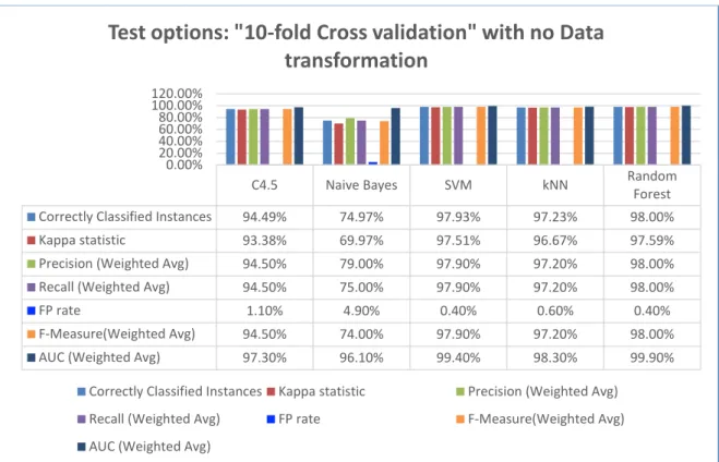
4.2.1. Experiment 1- Human Activity Recognition(HAR) ... 38
4.2.2. Experiment 2-Vehicle sensing ... 43
4.3.PERFORMANCE ANALYSIS RESULTS OF REGRESSION ALGORITHMS ... 48
4.3.1. Experiment 3- Appliance energy prediction ... 48
4.3.2. Experiment 4-Puma 560 robot arm ... 50
CHAPTER 5 ... 54
5.1T-TEST PERFORMANCE COMPARISON ... 54
5.1.1: T-test analysis of classification algorithms ... 55
5.1.2 T-test analysis of regression algorithms ... 57
CONCLUSION ... 59
REFERENCES ... 61
List of figures
FIGURE 2.1:ANALYTICS-DRIVEN SYSTEM DESIGN WORKFLOW ... 3
FIGURE 2.2:ARTIFICIAL NEURON COMPUTATIONAL MODEL ... 17
FIGURE 2.3:ANN ARCHITECTURE ... 18
FIGURE 2.4:SELF ORGANIZING MAPS ARCHITECTURE ... 20
FIGURE 2.5:ROCCURVE ... 27
FIGURE 3.1:CLASS DISTRIBUTION OF HARDATASET ... 30
FIGURE 3.2:CLASS DISTRIBUTION OF VEHICLE DATASET ... 31
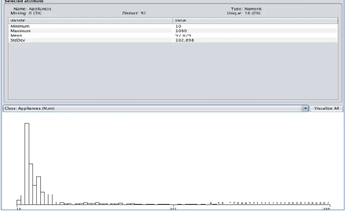
FIGURE 3.3:CLASS DISTRIBUTION OF APPLIANCES ENERGY PREDICTION DATASET ... 33
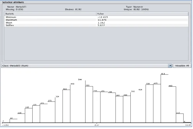
FIGURE 3.4:CLASS DISTRIBUTION OF PUMA 560 ROBOT ARM DATASET ... 34
FIGURE 3.5:SAMPLE ARFF FILE ... 35
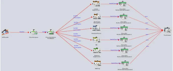
FIGURE 3.6WEKACLASSIFICATION TESTBENCH ... 36
FIGURE 3.7WEKA REGRESSION TESTBENCH ... 36
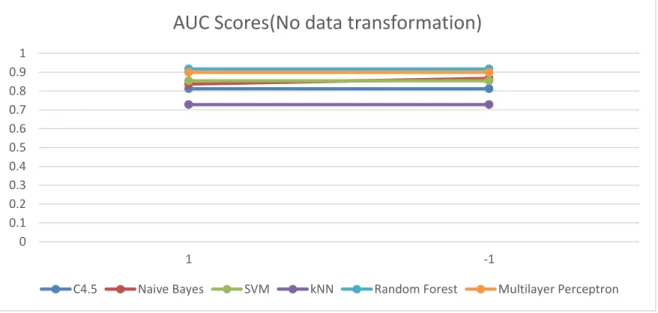
FIGURE 4.1:PERFORMANCE ANALYSIS REPORT ON HAR DATASET WITH NO DATA TRANSFORMATION ... 39
FIGURE 4.2 AUC SCORE 2D-LINE CHART FOR HAR DATASET WITH NO DATA TRANSFORMATION ... 39
FIGURE 4.3:1PERFORMANCE ANALYSIS REPORT ON HAR DATASET TRANSFORMED WITH RANDOM PROJECTION ... 40
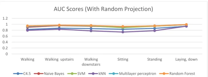
FIGURE 4.4AUC SCORE 2D-LINE CHART FOR HAR DATASET TRANSFORMED WITH RANDOM PROJECTION ... 40
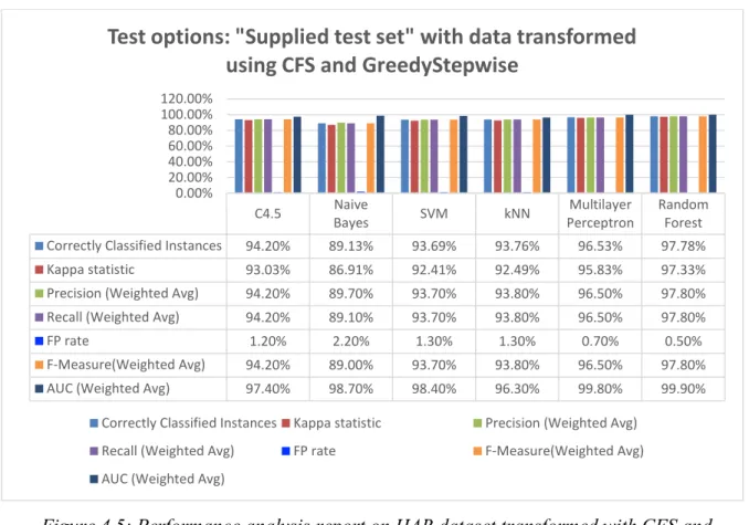
FIGURE 4.5:PERFORMANCE ANALYSIS REPORT ON HAR DATASET TRANSFORMED WITH CFS AND GREEDYSTEPWISE .... 41
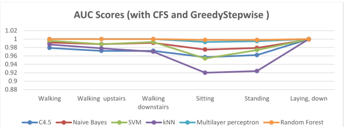
FIGURE 4.6:AUC SCORE 2D-LINE CHART FOR HAR DATASET TRANSFORMED WITH CFS AND GREEDYSTEPWISE ... 42
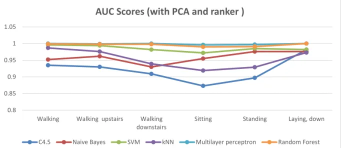
FIGURE 4.7:PERFORMANCE ANALYSIS REPORT ON HAR DATASET TRANSFORMED WITH PCA AND RANKER ... 42
FIGURE 4.8:AUC SCORE 2D-LINE CHART FOR HAR DATASET TRANSFORMED WITH PCA AND RANKER ... 43
FIGURE 4.9:PERFORMANCE ANALYSIS REPORT ON VEHICLE DATASET WITH NO DATA TRANSFORMATION ... 44
FIGURE 4.10:AUC SCORE 2D-LINE CHART FOR VEHICLE DATASET WITH NO DATA TRANSFORMATION ... 44
FIGURE 4.11:PERFORMANCE ANALYSIS REPORT ON VEHICLE DATASET TRANSFORMED WITH RANDOM PROJECTION ... 45
FIGURE 4.12:AUC SCORE 2D-LINE CHART FOR VEHICLE DATA TRANSFORMED WITH RANDOM PROJECTION ... 45
FIGURE 4.13:PERFORMANCE ANALYSIS REPORT ON VEHICLE DATASET TRANSFORMED WITH CFS AND GREEDYSTEPWISE ... 46
FIGURE 4.14:AUC SCORE 2D-LINE CHART FOR VEHICLE DATA TRANSFORMED WITH CFS AND GREEDYSTEPWISE ... 46
FIGURE 4.15:PERFORMANCE ANALYSIS REPORT ON VEHICLE DATASET TRANSFORMED WITH PCA AND RANKER ... 47
FIGURE 4.16:AUC SCORE 2D-LINE CHART FOR VEHICLE DATA TRANSFORMED WITH PCA AND RANKER ... 47
FIGURE 4.17:PERFORMANCE ANALYSIS REPORT ON ENERGY DATASET WITH NO DATA TRANSFORMATION ... 48
FIGURE 4.18:PERFORMANCE ANALYSIS REPORT ON ENERGY DATASET TRANSFORMED WITH RANDOM PROJECTION ... 49
FIGURE 4.19:PERFORMANCE ANALYSIS REPORT ON ENERGY DATASET TRANSFORMED WITH CFS AND GREEDYSTEPWISE ... 49
FIGURE 4.20:PERFORMANCE ANALYSIS REPORT ON ENERGY DATASET TRANSFORMED WITH PCA AND RANKER ... 50
FIGURE 4.21:PERFORMANCE ANALYSIS REPORT ON PUMA 560 ROBOT ARM DATASET WITH NO TRANSFORMATION ... 51
FIGURE 4.22::PERFORMANCE ANALYSIS REPORT ON PUMA 560 ROBOT ARM DATASET TRANSFORMED WITH RANDOM PROJECTION ... 51
FIGURE 4.23:PERFORMANCE ANALYSIS REPORT ON PUMA 560 ROBOT ARM DATASET TRANSFORMED WITH CFS AND GREEDYSTEPWISE ... 52
FIGURE 4.24:PERFORMANCE ANALYSIS REPORT ON PUMA 560 ROBOT ARM DATASET TRANSFORMED WITH PCA AND RANKER ... 53
FIGURE 5.1WEKAEXPERIMENTER ... 55
FIGURE 5.2:PAIRED T-TEST “PERCENT_CORRECT” ANALYSIS RESULTS OF CLASSIFIERS ON ORIGINAL HAR AND VEHICLE DATASET ... 56
FIGURE 5.3:PAIRED T-TEST “PERCENT_CORRECT” ANALYSIS RESULTS OF ALGORITHMS ON HAR AND VEHICLE DATASET TRANSFORMED WITH CFS AND GREEDYSTEPWISE. ... 56
FIGURE 5.4:PAIRED T-TEST “RMSE” ANALYSIS OF ALGORITHMS ENERGY DATASET ... 57
FIGURE 5.5:PAIRED T-TEST “CORRELATION COEFFICIENT” ANALYSIS OF ALGORITHMS ENERGY DATASET ... 57
FIGURE 5.6:PAIRED T-TEST “RMSE” ANALYSIS OF ALGORITHMS PUMA8NH DATASET ... 58
List of tables
TABLE 3.1:HAR DATASET CHARACTERISTICS ... 30
TABLE 3.2:VEHICLE SENSING DATASET CHARACTERISTICS ... 31
TABLE 3.3:APPLIANCES ENERGY PREDICTION DATASET CHARACTERISTICS ... 32
TABLE 3.4:PUMA 560 ROBOT ARM DATASET CHARACTERISTICS ... 33
List of acronyms
RFID Radio Frequency Identification
IoT Internet of things
XML Extensible Markup Language
HDF Hierarchical Data Format
CAN Controller Area Network
WSN Wireless Sensor Networks
TBDCS Tree-Based Data Collection Scheme
FNS Forwarding Nodes Set
MDL Minimum Description Length
WEKA Waikato Environment for Knowledge Analysis
SVM Support Vector Machines
kNN k-Nearest Neighbor
CV Cross Validation
IG Information gain
ID3 Iterative Dichotomiser 3
RF Random Forest
ANN Artificial Neural Networks
TP True Positive
TN True Negative
FN False Negative
FP False Positive
ROC Receiver Operating Characteristic
AUC Area Under the Curve
WSDN Wireless Distributed Network
HAR Human Activity Recognition
RMSE Root Mean Square Error
MAE Mean Absolute Error
ARFF Attribute-Relation File Format
CLI Command Line Interface
RBF Radial Basis Function
DELVE Data for Evaluating Learning in Valid Experiments
Chapter 1
1.1 Introduction
“Information is the oil of the 21st century, and analytics is the combustion engine”
Peter Sondergaard, Gartner
Integration of embedded systems into the field of electronics design has been increasingly ubiquitous, ranging from modern everyday appliances like mobile phones, Radio Frequency Identification (RFID) tags in home appliances, modems, remote controls, watches etc. to complex system development like automobiles, space researches, power plants etc. Internet of things (IoT) has also emerged as an evolving technology which has found its place in embedded electronics domain. With the rapid growth and advancement in IoT and embedded electronics, a network of interconnected devices has been created, which has revolutionized the concept of networking and data communication but it comes with a price, the challenge of handling the massive amount of data these interconnected applications generate. With increasing demand for energy efficient, reliable, scalable and faster applications, the need for turning data into useful information and knowledge has attracted a great deal of attention in the research community, which has led to the emergence of analytics-driven system design.
Designers combine the data mining techniques into the embedded system design to make the application context-aware and be able to predict the system's behavior. The implementation of analytics differ depending on the system usage, in some cases, the analytics is performed in the cloud to improve the embedded-systems performance while in some it runs directly in the embedded system. The initial step in the direction of analytics design is the selection of the appropriate data mining technique to ensure system robustness, reliability and efficient cost management in the architecture, design, and maintenance.
In this thesis, a qualitative comparative analysis of state-of-art data mining algorithms using datasets generated by embedded devices is presented. The objective of this study is to identify the optimal data mining models specific to the dataset.
1.2 Organization of thesis
The rest of the thesis has been organized as follows. Chapter 2 focuses on the theoretical foundations of analytics-driven embedded system design. The first part of the chapter covers the generalized workflow of the analytics design for embedded systems, here different steps and the tasks performed during the process is explained. The second part of the chapter covers the basic concept and principle of the state-of-art machine learning algorithms. In chapter 3, dataset chosen for the study and the toolkit used are described and an overview of the experimental setup is illustrated. Chapter 4 covers experimentation in detail and initial result of the analysis. Finally, in chapter 5 the t-test analysis results are scrutinized and concluding remarks are presented.
Chapter 2
2.1. Workflow in analytics-driven system design
Typically, the process of data mining starts with problem definition which sets the path for data modeling. The key aspects of a problem definition are clarity of the business requirement and a cost/benefit estimate [9]. Knowledge of business requirement and the way data can be used to achieve the desired goal is the stepping stone in the process of analytics. The next significant step is the collection of data which determine the rest of the step to be followed in the data modeling. A pictorial representation of the sequence of steps designers follow to build an embedded system analytics model to accomplish the expected outcome is shown in Figure 2.1.
Figure 2.1: Analytics-driven system design workflow
2.1.1. Data collection
Applying a systematic approach to collecting the raw data is foundation step in the workflow. In embedded computing domain, data is being collected from a varied range of sources and in distinct forms. For smart devices embedded with electronics, software, sensors, actuators, each event detection generate data and can be of various formats such as text, spreadsheet, image, audio, video, geospatial, web, Extensible Markup Language(XML) and Hierarchical Data Format (HDF) for scientific data, and Controller Area Network (CAN) for automotive data. Data from multiple sources must be integrated and stored so that it is accessible for training the model. In case the IoT devices, multiple devices are part of a Wireless Sensor
Networks (WSN) creating a massive volume of data. Data collection schemes in devices connected through WSN or any embedded devices that operate in-situ must fulfill following objectives: a) minimal energy consumption, b) minimized latency and c) optimized CPU usage [3].
Different data collection methodologies have been proposed keeping the mentioned goals in mind. Data aggregation is a basic operation in WSN since it is typically restricted in hardware infrastructure and communication recourses. Tree-based technique and cluster-based technique are the two most commonly used data collection methodologies adopted in embedded systems analytics workflow. As proposed in [4], Tree-Based Data Collection Scheme(TBDCS) is a distributed data collection method which establishes a tree structure with intermediate nodes termed as Forwarding Nodes Set(FNS). These intermediate nodes act like data aggregators to transmit data from sensor nodes back along the tree. Through different simulations and scrutiny, it has been inferred that TBDCS significantly reduces transmission latency and network congestion.
Cluster-based data collection method has been claimed to be effective in systems which are limited in energy consumption and network bandwidth [5]. In this technique, a cluster head is designated among a group of sensor nodes and similarly multiple disjoints sets are formed with a group of sensor nodes. Sensors in the cluster send information to the cluster head, The cluster head suppresses the local redundancies and communicates the compressed data to the main system. In this process, the cost of sending redundant data is reduced thereby preserving energy and minimizing the scalability constraint.
Another challenge of data collection is the structure of data that determine various characteristics of the dataset such as multivariate, sequential, time-series, image signals etc. In addition to that, each dataset can contain a heterogeneous list of attributes. All these aspects of data steer the choice of machine learning technique to be used for analysis.
2.1.2. Data pre-processing
The bitter truth of data science is the data collected from real-world applications are not machine learning ready. Real data is low in quality in terms of completeness, accuracy, and consistency, hence unreliable to be used to design an intelligent analytics model. The data
processing the data has become the most essential and expensive step in the data mining workflow. Due to growing demand for smart systems with multiple data generating nodes, designing a reliable and high performing predictive model has become paramount. Pre-processing is part of the iterative data mining workflow and are optimized by multiple runs of the workflow and are greatly determined by the statistics generated by the algorithms used to train the data. One must undergo different phases of data pre-processing to achieve a predictive data model.
The first stage of preparing the data is to understand the features of the raw data to identify outliers, noise etc. Descriptive data summarization reveals the raw data characteristics. Measurement of central tendency and dispersion of data are standard techniques used to describe the anomalies in data. Mean, median, mode, and midrange are properties that define the central tendency of a dataset and measures of quartiles, interquartile range and variance determine how disperse the data is [7]. During this process, the main features of the data can be identified which are essential for proceeding to the next stages [6]
Another phase of preparing the data is feature selection. Raw data contain magnitude of attributes and it is crucial to filter out those attributes which do not have a relevant contribution to the machine learning process. Discretization is one way of transforming the data to suit some of the specific classification and clustering algorithms. In this process, a large number of data values (numeric attributes) are converted into a smaller number of discrete values. These methods are used for attribute reduction by grouping the continuous attributes into a range of values. Applying discretization to data enhances the predictive accuracy and boost the performance as well. Discretization algorithms can be categorized as boolean reasoning, equal frequency binning, entropy-based discretization [7]. Depending on the complexity of the raw data, additional data transformation is needed to optimize the training process. Projection is one of the technique used to project training data such as spatial data in lower dimensional spaces, but still preserves the inherent relationships in the data. Principal component analysis another way of transforming data into a set of values of linearly uncorrelated variables called principal components. Section 2.2 covers the details of some of the popular pre-processing algorithms.
After the data has passed the initial pre-processing stage, mining model is built using the transformed data and machine learning algorithms. This model forms the base to extract patterns. Discovery of patterns is mainly determined by the selection of training data, type of algorithms used and how the algorithm is configured[8]. Different dataset require specific machine learning tasks, for example, deep learning algorithms should be used in case of complicated dataset like face recognition, time-series datasets like sensor data from wearable devices need clustering and classification learning models, multivariate dataset like appliances energy prediction data, forest fire data etc. might work best with regression learning tasks.
Classification
Classification machine learning is used to predict discrete data points or class labels for the data instance based on the prediction model called classifier. A classifier is constructed by training on the dataset through a series of machine learning tasks. The simplest classification type is of a binary class labeled data model. In binary classification the observed instance can only be categorized into two class labels. Classification algorithms find relationship between the value the attributes which are identified as predictors and a discrete output value such as color, type or true/false, using the training set. The model is designed based on these relationships and then applied to the real time dataset to predict the class label.
Regression
Regression data modeling determine relationships between the value the attributes which are identified as predictors and a continuous output value. A continuous output variable is a real-value, such as an integer or floating point value such as size, amount etc. There are several machine learning algorithms which can be used for both regression and classification such as decision trees, support vector machine and artificial neural networks but there some specific algorithms which are only meant for regression like linear regression and addictive regression.
Clustering
Clustering is used when the class label is unknown or not certain. The aim is to segregate dataset instances with similar traits into groups and categorize them into clusters by dividing the data instances in the dataset into a number of groups such that data points within a group are more similar to other data points in the same group than those in other groups.
A mining model is generated by performing a series of adjustments to the algorithms and data creating different results which are then evaluated and compared to select the optimal analytics setup. During this process, both the mining structure and mining model are updated after each adjustment. Dataset structure mainly consists of data source definition, list of instances and list of features. A mining model architecture consists of metadata, data mining results in form of patterns and a data binding structure to the original data. The metadata gives the specifics of the model such as the name of the model, mining structure used for the model, machine learning algorithms used to analyze the data. Each model is characterized by two properties. Algorithm property defines the algorithm that is used to create the model. It can be set during the data analysis phase and can be changed later but the model must be reprocessed to generate the accurate pattern. Another property is the usage which specifies how each attribute is used by the model [8].
Each machine learning task has a varied range of algorithms which can be used in combination to create an intelligent data analysis model. Section 2.2 covers the concepts of some of the state-of-art algorithms.
2.1.4. Data evaluation
Data evaluation is the key step to ensure the credibility of a model and is a cumbersome process. Data evaluation begins by setting up a systematic evaluation method to explore how different models structure the data and do a comparative analysis. Selection of a discrete test data set is pre-requisite for trustworthy evaluation since performance on the training set is not a good indicator of future performance. The reason is that the model has been trained from the very same training data and an estimate of performance based on that data will be optimistic and not realistic.
Over the years, different evaluation methods have been proposed for different category of data mining models. Cross-validation, hold out and random subsampling and bootstrap are the most commonly used methods for classification and regression models. Evaluation schemes assess the performance on multiple metrics such as sensitivity and specificity, precision, kappa statistics, mean absolute error, root mean squared error, relative absolute error and root relative squared error. Cross-validation is the preferred method of choice of data scientists. For clustering schemes, Minimum Description Length(MDL) is considered for evaluation. To
find the best data mining algorithm to design the data model, a comparative analysis is needed to predict the true performance of different algorithms. The t-test is commonly used to perform such experimentation. Details of the evaluation schemes used in this study have been covered in section 2.2. However MDL is beyond the scope of this study and hence not covered.
2.1.5. Model deployment
The last step in the data mining process is to integrate the analytics model into a commercial environment. The model can then be used to perform multiple tasks such as real-time object detection, tracing patterns from new signals, making predictions to direct business decisions, creating queries to retrieve new patterns, rules, and behavior.
2.2. Conceptual overview of data mining algorithms
2.2.1. Data transforming algorithms
Feature selection
Feature selection is a form of data reduction where irrelevant, or redundant attributes can be detected and removed. Algorithms are categorized into a scheme-independent selection (filter method) and scheme-specific selection (Wrapper method) [10]. In WEKA interface, the process of attribute selection is split into two parts: (a) attribute evaluator- the process of assessing the selected attribute subset (b) search method- the process of searching a possible subset.
2.2.1.1. Ranker
This algorithm works on the principle of information gain attribute ranking. It is one of the simplest attribute selection method which ranks attributes by their individual evaluations and mostly used in decision tree classifiers like C4.5 classifier. Information gain(IG) is based on entropy metrics. The entropy measure is a measure impurity and can be calculated as H(X)
H(X) = − ∑ p(xi) log2( p(xi))
n
i=1
( 2.1)
where p(x) is the marginal probability density function of a discrete random variable X with N outcomes. IG is measured by the amount of information gained by splitting the dataset using the chosen attribute whereas entropy of the class reflects the attribute contribution in gaining clear information about a class. Attributes are ranked based on IG value, where attributes with high scores are selected since they can be used for better prediction [10] [11].
2.2.1.2. Correlation-based Feature Selection (CFS)
Correlation-based Feature Selection method evaluates a subset of attributes instead of assessing individual attributes. Efficacy of individual features is considered for predicting the class along with the degree of inter-correlation among them. High scores are assigned to subsets containing attributes that are highly correlated with the class and poorly inter-correlated with each other. Scores are measured by heuristic merits formulated by the Equation 2.2 (Ghiselli 1964) [12].
𝑟𝜃𝑆 = 𝑘𝑟𝜃𝑖
√𝑘 + 𝑘(𝑘 – 1)𝑟𝑖𝑗 ( 2.2 ) where rθs is the score of the subset, rθi is the average correlation between the k variable and
θ, and rij is the average of attribute subset intra-correlation.
2.2.1.3. Greedy stepwise
Greedy stepwise method selects the attributes by performing a forward or backward search through the attribute subspace which can be random. During the process of search the greedy stepwise method creates a ranked list of attributes and the search process stops when the addition or deletion of any remaining attributes results in a decrease in evaluation. Greedy stepwise feature search is used in conjunction with CFS in WEKA.
Discretization
As mentioned in section 2.1, discretization is mainly needed for datasets with continuous numeric attributes and can be achieved by sorting all the continuous values of the attribute
and splitting continuous values into a predetermined number of equal intervals (unsupervised discretization) or using the number of classes as the discretization parameter (supervised discretization). Unsupervised discretization methods are only suitable for clustering type of training where the class is non-existent or uncertain [7].
2.2.1.4. Boolean reasoning
Boolean reasoning builds on the Boole-Schröder algebra of logic, which is based on Boolean equations with predicates which are true or false. It is a straightforward implementation that filters a small subset of attribute values that do not preserve the discernibility. The remaining subset is a minimal set of cuts preserves the discernibility inherent in the dataset. The algorithm operates by first creating a Boolean function from the set of candidate cuts, and then computing a prime implicate of the Boolean function [7].
2.2.1.5. Entropy-based discretization
It is a form of supervised discretization which based on the MDL principle as described in [11]. Several entropies-based algorithms have been proposed which work for multiple domains. Some algorithms work on the principle of recursively partitioning the value set of each attribute so that the local measure of entropy is optimized and some are based on maximizing the entropy over discretization space [13].
Feature extraction
Also known as dimensionality reduction, feature extraction is a process of transforming the high dimensional dataset to a reduced or compressed representation of the original data before starting the modeling process. During the process of feature extraction, the original data can be either be transformed without losing any information (lossless data reduction) or the transformed data approximates the original data (lossy data reduction) [1]. In realistic data mining process, lossy data reduction is the typical outcome of as dimensionality reduction. Several algorithms have been invented for this purpose out which PCA and Random Projections are the preferred ones.
Principle Component Analysis(PCA) is a mathematical procedure which is based on projection principles. In this method, an orthogonal restructuring of a high dimensional data set to a set of values of linearly uncorrelated variables called principal components. PCA was developed and named by Harold Hotelling in 1930 which was based on the algorithm derived by Karl Pearson as an analog of the principal axis theorem in 1901[14]. PCA is done by deriving a covariance matrix of a data set consists of covariance values between all the different dimensions. Covariance indicates the relationship between two dimensions and can be calculated as 𝐶(𝑋, 𝑌) =∑ (𝑋𝑖 − 𝑋 𝑛 𝑖=1 )(𝑌𝑖 − 𝑌) 𝑛 − 1 ( 2.3 )
where C is the covariance and X and Y are the two dimensions of a dataset which has n number of instances and 𝑋, 𝑌 are the mean of the dimension X and Y. For an N-dimensional
data set, covariance matrix will have (𝑁−2)!∗2𝑁! a number of covariance values. Then the eigenvectors and eigenvalues of the covariance matrix are calculated and eigenvectors are normalized so that the length is always 1 The eigenvectors are then ranked according to the eigenvalues. The eigenvectors which have high scores are selected as principal components. The transformed data is derived from the original dataset by using the set of selected principal components called a feature vector, formulated in Equation 2.4.
𝐷𝑓𝑖𝑛𝑎𝑙 = 𝐹𝑉𝑡𝑟𝑎𝑠𝑝𝑜𝑠𝑒𝑑× 𝑀𝐷𝑜𝑟𝑔𝑡𝑟𝑎𝑛𝑠𝑝𝑜𝑠𝑒𝑑
( 2.4 ) where FV is the feature vector matrix which row transposed and MDorgtransposed is the transposed matrix of mean adjusted values of the original dataset i.e. the data items are in each column, with each row holding a separate dimension [15].
2.2.1.7. Random Projection
Another technique of feature extraction is Random Projection(RP) where the original data is projected onto a predefined lower dimensional subspace using a random matrix whose columns have unit lengths. In RP, the original d-dimensional data is projected to a k-dimensional (k << d) subspace through the origin, using a random (k × n) matrix R whose columns have unit lengths. RP can be formulated in the Equation 2.5.
𝐷𝑘×𝑁𝑅𝑃 = 𝑅
𝑘×𝑑 × 𝐷𝑑×𝑁 ( 2.5 )
where 𝐷𝑑×𝑁is the original set of N n-dimensional instances, 𝐷𝑘×𝑁𝑅𝑃 is the projection of the data onto a lower p-dimensional subspace. The key idea of random mapping arises from the Johnson-Lindenstrauss lemma [16] which states that distance relationships are preserved quite well on an average. Random projection implementation can be done in different ways. One is based on Gaussian distribution [17] and other implements a sparse random matrix as proposed by Achlioptas in [18].
2.2.2. Data mining algorithms
Machine learning algorithms are typically categorized into supervised and unsupervised algorithms based on the training dataset characteristics. A supervised method of learning can be applied to the dataset where the output (the desired result) is one of the attributes in the training dataset. Classification and regression algorithms are used for those cases. Classification models are based on predicting discrete class attribute value or a probability for a class attribute value whereas regression modeling is used to predict a continuous quantity which can be a real value or discrete integer variable. There are few algorithms which can be used for both classification and regressing modeling such as neural networks, decision trees but algorithms like linear regression and additive regression can be used only for regression type. Unsupervised algorithms are used in those cases where the output attribute is unknown or non-existent in the training dataset. Clustering is the most common technique used in unsupervised algorithms.
2.2.2.1. C4.5
C4.5 is an algorithm used for classification by generating decision trees. It was developed by Ross Quinlan as an extension to the Iterative Dichotomiser 3 (ID3) algorithm [2]. C4.5 is the most popular algorithm used for classification type data modeling. The basic principle of C4.5 involves building decision trees on the training data using the information gain entropy principle for attribute selection as explained in section 2.2.1.1.The attribute with the highest normalized information gain is chosen to make the decision. The C4.5 algorithm then recurs on the smaller partitioned data. Usually, a fully expanded decision tree reveals irrelevant structure so pruning method is applied. Pruning can be either forward pruning which is done
during the decision tree creation, or it can be backward pruning which is done after the decision tree has been built. C4.5 uses a backward pruning method by default. In some cases pruning causes a fall in the accuracy of the model prediction, thereby correct estimation of error rates is significant. C4.5 uses a default confidence level of 25% to calculate the error rate e in Equation 2.6 [2]. 𝑒 = 𝑓 + 𝑧2 2𝑁 + 𝑧√𝑓𝑁 −𝑓 2 𝑁 + 𝑧 2 4𝑁2 1 +𝑧𝑁2 ( 2.6 )
where N is the number of samples and f is the observed error rate and z is the number of standard deviation which is calculated using the confidence level.
2.2.2.2. Naïve Bayes
Naïve Bayes machine learning algorithm is a type of statistical classifier and is based on
Bayes’ theorem which works on the principle of conditional probability. In a practical
scenario, datasets have many attributes therefore, use of simple Bayes' theorem would be computationally expensive, so Naïve Bayes makes an assumption of class conditional independence which means there are no dependency relationships among the attributes. Naïve Bayes classifier predicts that the data instance X belongs to a class if and only if,
𝑃(𝐶𝑖|𝑋) > 𝑃(𝐶𝑗|𝑋) 𝑓𝑜𝑟 1 ≤ 𝑗 ≤ 𝑚, 𝑖 ≠ 𝑗 ( 2.7 )
where 𝑃(𝐶𝑖|𝑋) is the probability of X belonging to class 𝐶𝑖 , assuming that the training dataset has m classes. 𝑃(𝐶𝑖|𝑋) is calculated as
𝑃(𝐶𝑖|𝑋) = 𝑃(𝑋|𝐶𝑃(𝑋)𝑖)𝑃(𝐶𝑖)
( 2.8 )
where 𝑃(𝑋) is the prior probability of X which is a constant value, 𝑃(𝐶𝑖) is the prior
probability of 𝐶𝑖 independent of its attribute values. 𝑃(𝑋|𝐶𝑖) is the posterior probability of X
𝑃(𝑋|𝐶𝑖) = ∏ 𝑃(𝑥𝑘|𝐶𝑖)
𝑛
𝑘=1
( 2.9 )
where 𝑥𝑘 refers to the value of attribute 𝐴𝑘for instance X. In case of a continuous attribute value, 𝑃(𝑋|𝐶𝑖) is calculated using the Gaussian distribution of the attribute value [1].
2.2.2.3. Random Forest
Random Forest(RF) is an ensemble machine learning method best suited for classification and regression tasks. An ensemble machine learning is a combination of multiple classifiers to get a better predictive efficiency. There are different types of ensemble methods such as error-correcting output coding, bagging, boosting and randomization[27]. RF algorithm was first developed by Leo Breiman [26] by combining his concept of bagging [28] and random subspace method introduced by Tin Kam Ho [29]. Leo Breiman defines RF as “A random
forest is a classifier consisting of a collection of tree-structured classifiers {ℎ(𝑥, Θ𝑘), 𝑘 =
1, … } where the { Θ𝑘} are independent identically distributed random vectors and each tree cast a unit vote for the most popular class at input x” [26]. As described by Leo Breiman in
[26] the error rate of random forest classification is dependent on correlation between any two trees in the forest. The error rate is directly proportional to correlation. RF is claimed to be an efficient machine learning method when a dataset is large and there is a high risk of overfitting due to missing data[26].
2.2.2.4. k-nearest neighbor(kNN)
k-nearest neighbor classifier is one of the basic classification technique used when the estimation of the parametric probabilities is not an easy process. It belongs to the family of instance-based machine learning methods. kNN was first proposed by Fix & Hodges in 1951. In kNN a lazy learning approach where the actual processing is done when a test instance is applied to the classification model. Assuming that the training dataset is described by n attributes, a k-nearest-neighbor classifier searches for patterns between the test data instance and the k training data instances based on the closeness in distance metrics. The distance metric, usually Euclidean distance between a test sample 𝑋1 = (𝑥11, 𝑥12, 𝑥13… 𝑥1𝑛 ) and the
given training samples 𝑋2 = (𝑥21, 𝑥22, 𝑥23… 𝑥1𝑛) is taken into consideration to determine the closeness and can be calculated as Equation 2.10.
𝐷𝑖𝑠𝑡(𝑋1𝑋2) = √∑(
𝑛
𝑖=1
𝑥1𝑖 − 𝑥2𝑖)2 ( 2.10 )
kNN in its original form perform poorly in terms of accuracy due to its inherent property of assigning equal weight to the attributes, so the application of data transformation methods prior to classification modeling is imperative. kNN classifier also lacks in speed since it requires an iterative process to spot the K training instance. Transforming the training data into sorted search trees and employing parallel execution reduces the comparison time[1].
2.2.2.5 Linear Regression
Linear regression method is typically used for modeling dataset with numeric attributes and numeric class prediction. Linear regression models assert response variable 𝑦𝑖 as a linear
function of 𝑥𝑖 is the weighted attribute value. 𝑦𝑖 for 𝑖𝑡ℎinstance can be calculated as
𝑦𝑖 = 𝑤0+ ∑ 𝑤𝑗𝑥𝑗
𝑘
𝑖=1 ( 2.11 )
where 𝑤0 , 𝑤𝑗are the weights which are used as regression coefficients and are computed by
the least square method to find the best fitting values which minimize the difference between the actual class and the predicted class 𝑦𝑖. The overall minimization can be calculated by
taking the sum of squares of differences for all instances and the goal is to have a minimum value for better prediction accuracy. Linear regression models are limited to datasets which exhibit linear dependency and only support regression type problems [1][2].
2.2.2.6 Gradient Boosting Machines (GBM)
Gradient boosting works on the notion of a week classifier can be enhanced to give better results. Friedman introduced the Gradient Boosting Machines to conceptualize this idea[41]. Elements involved in gradient boosting are loss function such as least square that is optimized during the learning process, a base learner such as decision tree ,which makes the predictions and an addictive model to which the base learner is sequentially fitted in order to minimize
the loss function. Friedman in [41] analyses that accuracy and the execution speed of gradient boosting can be enhanced by adding randomization to the sampling procedure. For a given training sample D {𝑦𝑖, 𝑥𝑖}𝑁 where X is the set of attributes, the goal is to find a function 𝐹∗(𝑥) that maps x to 𝑦 such that over the joint distribution of all values, the expected value of some
specified loss function ψ(𝑦, 𝑓(𝑥)) is minimized as shown in Equation 2.12. 𝐹∗(𝑥) = 𝑎𝑟𝑔 𝑚𝑖𝑛
𝐹(𝑥)𝐸𝑦,𝑥 𝜓(𝑦, 𝑓(𝑥)) ( 2.12) Boosting constructs the addictive model by approximating 𝐹∗(𝑥) as shown in Equation 2.13.
𝐹(𝑥) = ∑ 𝛽𝑚
𝑀
𝑚=0
ℎ(𝑥; 𝑎𝑚)
( 2.13)
where ℎ(𝑥; 𝑎𝑚) is the base learner with parameters 𝑎 = {𝑎1, 𝑎2, … 𝑎𝑚} and 𝛽𝑚 is the expansion coefficient and M is the number of iterations.
The generic gradient boosting is greedy algorithm this prone to overfitting . To minimize the overfitting some parametric modification such as tree depth, learning rate and number of random samples can be done in the algorithm. It is a common practice to have the tree depth between 4-8 levels and learning rate between 0.1 to 0.3.
2.2.2.7. Support Vector Machines (SVM)
Support Vector Machines is one of the most popular machine learning algorithm which is
widely used for both classification and regression modeling tasks. The reason for SVM’s high
acclamation is its capability to provide a robust and efficient algorithm which can handle both linear and nonlinear data. The standard algorithm that is widely used today was proposed by Corinna Cortes and Vapnik in 1993 but its origin dates back to 1963 [32]. The basic principle of SVM is to construct a set of hyperplanes called support vectors and then a linear model is built on the nonlinear hyperplanes. In case of a two-class learning task, the goal is to identify the best classification function to separate data instances in the training dataset. The separation function corresponds to a hyperplane separating dataset into two classes. In SVM, the best separating hyperplanes can be identified by maximizing the margins between the classes. Margin can be deduced geometrically as the shortest distance between the nearest
data points called support vectors, to the hyperplane. The maximum margin hyperplanes can be defined by Equation 2.14[2] 𝑥 = 𝑏 + ∑ 𝛼𝑖𝑦𝑖 𝑖 𝑖𝑠 𝑡ℎ𝑒 𝑠𝑢𝑝𝑝𝑜𝑟𝑡 𝑣𝑒𝑐𝑡𝑜𝑟 (𝑎𝑖 ∙ 𝑎) (2.14)
where 𝑦𝑖 is the class label, 𝑎𝑖 ∙ 𝑎 is the dot product of training data vector 𝑎𝑖 and test data
vector 𝑎, 𝛼𝑖 and b are coefficients determined during the training process using constrained
quadratic optimization. In case of the nonlinear dataset, the hyperplane function can be derived by extending the dot product 𝑎𝑖∙ 𝑎 to a kernel functional mapping Φ𝑎𝑖∙ Φ𝑎 where Φ is the function that projects the data into a transformed higher dimension [2].
Several kernel functions have been proposed in recent years which optimizes the SVM classification. To handle multiclass classification, the coefficient 𝛼𝑖 is generalized. Many
variations of SVM have been proposed to handle different machine learning tasks. LIVSVM is an open source library which was developed by Chang, Chih-Chung; Lin, Chih-Jen in 2000[33], which includes support vector classification, regression and one-class SVM.
2.2.2.8. Artificial Neural Networks
Artificial Neural Networks (ANN) are complex data modeling systems which are inspired by the core concept of biological neurons. An ANN is composed of connected input/output processing unit each with an associated weight. The individual units are called nodes or neurons and are based on the basic computation model proposed by McCulloch and Pitts as shown in Figure 2.2.
Figure 2.2: Artificial neuron computational model
The output can be mathematically computed in Equation 2.15 as the weighted sum of its n input signals, 𝑥𝑗={1,2,….𝑛} and it generated the output as 1 if the weighted sum is above a
𝑓(𝑥) = 𝜃 (∑ 𝑤𝑗
𝑛
𝑗=1
𝑥𝑗 − 𝑢) (2.15)
where 𝜃(. ) is the activation or transfer function, 𝑤𝑗 is the weight of the input. The purpose of activation function is to non-linearize the neural network and generalize the neurons. The basic architecture of ANN consists of layers of interconnected neurons and connections with associated weights as shown in Figure 2.3. Performance is improved over time by iteratively updating the weights in the network.
Figure 2.3: ANN architecture
Depending on the architecture, ANN can be categorized into feedforward or feedback(recurrent) networks. The process of learning in ANN involves updating the architecture and the connection weights. Feedforward networks are associated with supervised learning and feedback networks are associated with unsupervised learning. In feedforward network, there is an input layer, one or multiple hidden layers and an output layer and lines connecting the neurons have an associated weight with it as shown in the figure. The inputs to the network correspond to the attributes of training data instance.
Multilayer Perceptron
A multilayer perceptron is a class of feed-forward neural network and utilizes backpropagation algorithm for learning. During the training phase, backpropagation learns by iteratively processing the dataset instance and comparing the network output to the class
attribute value and subsequently adjusting the weight to reduce the mean squared error between the predicted value and actual value by using a gradient-descent method. The algorithm is called backpropagation because the adjustment is made in backward direction i.e. from the output layer down to hidden layers. The squared error in the 𝑗𝑡ℎnode of the output layer for a can be determined as
𝐸 =1
2∑(𝑦𝑗− 𝑓(𝑥𝑗))2
𝑗 ( 2.16)
Here y is the class label of the instance and f(x) is value produced by the output layer. With gradient descent, the connection weight of 𝑗𝑡ℎ and 𝑖𝑡ℎ neurons is adjusted by
∆𝑤𝑗𝑖 = −𝜂 𝑑𝐸
𝑑𝑔(𝑥𝑗)(𝑓(𝑥𝑖)) (2.17)
where 𝑓(𝑥𝑖) is the output of the previous neuron, 𝜂 is the learning rate and. The derivative
can be calculated as − 𝑑𝐸 𝑑𝑔(𝑥𝑗) = ∅′(𝑔(𝑥𝑗)) ∑ − 𝑘 𝑑𝐸 𝑑𝑔(𝑥𝑘)𝑤𝑘𝑗 ( 2.18 )
with ∅′ being the derivative of activation function and can be seen that the derivate depends on the depends on the change in weights of the 𝑘𝑡ℎ node in output layer and thus the change of weight in the hidden layer is the back propagated according to the derivative of the activation function [34].
Due to its capability to handle non-linearity and versatile nature, multilayer perceptron has its roots in varied machine learning tasks such as image recognition, speech recognition, regression modeling etc.
Self-Organizing Maps(SOM)
Self-Organizing Maps also known as Kohonen’s SOM, is a class of feedforward artificial
1984[35]. The principal objective of SOM is to define a high dimensional dataset in one or two-dimensional data space while preserving the topographic relationships of data. SOM has a single computational layer consisting of a grid of neurons arranged in rows and columns and an input layer consisting of an input vector. Each neuron in the computational layer is connected to all the source nodes in the input layer as shown in below Figure 2.4.
Figure 2.4: Self Organizing maps architecture
The process of generating the self-organizing maps begins by initiation the connection weights with a random value. A sample of the input vector is chosen from the training dataset. If the input vector has d dimension then it is represented as 𝑥𝑖 : 𝑖 ∈ {1,2 … . 𝑑} and the computational layer is constructed by N neurons mapped in (X, Y) dimension. Each input unit is connected to the neurons by connection weight 𝑤𝑗𝑖: 𝑗 ∈ {1,2, … 𝑁}. Next step is to find the
winning neuron, the one which has the weight vector closest to the input vector i.e. minimum value of discriminant function 𝑓(𝑥) . It is computed as
𝑓𝑗(𝑥) = ∑(𝑥𝑖
𝑑
𝑖=1
− 𝑤𝑗𝑖)2 ( 2.19 )
where 𝑓(𝑥) calculated by taking the square Euclidean distance between the input unit and
neuron. Once the winning neuron has been identified, a topological neighborhood is defined by considering the lateral distance between the neurons in the grid as formulated as Equation 2.20.
𝑇𝑗𝑊(𝑋) = 𝑒𝑥𝑝 (−
𝑆𝑗𝑊(𝑋)2 2𝜎2 )
(2.20 )
where 𝑆𝑗𝑊(𝑋) is the lateral distance between the neuron j and winning neuron W(X), 𝜎 is the
epoch which denotes the width of the neighborhood and programmed to exponentially decrease over time. Once the neighborhood is determined, the weight neurons in the neighborhood are updated by ∆𝑤𝑗𝑖.
∆𝑤𝑗𝑖 = 𝜂(𝑡)𝑇𝑗𝑊(𝑋)(𝑡)(𝑥𝑖 − 𝑤𝑗𝑖) (2.21 )
where t is the epoch dependent on learning rate 𝜂(𝑡) = 𝜂0exp (𝑡/𝜏𝜂). The update causes the
weight vectors of the winning neurons and the neighboring neurons to move towards the input vectors and this process is iterated for all training data instances to achieve a topographical convergence generating self-organizing feature maps which discretely represent the input data in a lower dimensional output space [35].SOM is also considered as a non-linear generalization of PCA due to its capability to cluster non-linear data instances.
2.2.2.9. K-mean
K-mean is a classic clustering technique based on iterative partitioning method. The standard algorithm was first proposed by Stuart Lloyd in 1957 as a technique of vector quantization in signal processing [31].The k-mean algorithm creates an initial partition of k (𝑘 ≤ 𝑛) clusters
from a dataset of n instances where each cluster is represented by the mean value of the instances in the cluster. In the second step, an iterative relocation technique is applied to the data observed by comparing the least squared Euclidean distance between the objects and the centroid and relocating the centroid. This process is repeated unit the squared error criterion converses. It can be defined as
𝐸 = ∑ ∑ |𝑝 − 𝑚𝑖 𝑝∈𝑐𝑖 𝑘 𝑖=1 |2 ( 2.22 ) where E is the sum of squared error of all instances in the dataset, p is a point in the multidimensional space in the cluster 𝑐𝑖 , 𝑚𝑖 is the mean of the cluster 𝑐𝑖 [1]. K-mean algorithm determines k partitions that minimize the square-error function and its efficiency is limited only to datasets which are clearly divergent. Additional data transformation is needful for fitting it to the real world dataset clustering.
2.2.3. Model Evaluation techniques
Designing an analytic model for the embedded system requires a thorough evaluation of the model in terms of cost and performance. As mentioned in section 2.1 , cross-validation and t-test are commonly used evaluation techniques.
2.2.3.1. Cross-validation
Cross-validation is the most commonly used method to evaluate predictive models by partitioning the original sample dataset into a training set to train the model, and a test set to evaluate it. It is mainly used to estimate the performance of the model through different metrics. The basic form of cross-validation is the k-fold cross validation where the original sample is randomly partitioned into k equal sized subsamples. k − 1 subsamples are used as
training dataset and 1 is used as test dataset to perform the prediction of the model trained using the training dataset. Cross-validation process is repeated K times with of the data sub-samples used exactly once for creating the test data and an average of K then k results from the folds gives a single estimation [20]. The estimation is measured in terms of prediction accuracy as proposed in Equation 2.23 [19].
𝑎𝑐𝑐𝑐𝑣 =1
𝑛 ∑ 𝛿(𝐼(𝐷 ∖ 𝐷𝑖, 𝑣𝑖), 𝑦𝑖)
𝑣𝑖𝑦𝑖∈𝐷
( 2.23 )
where D is the sample dataset which is randomly split into K folds. The model is trained on
D ∖ Dt subsample where t ∈ {1,2 … k}. Di is the test data sample with instance xi = (viyi). The overall cross-validation is average of (m/km ) possibilities for m/k instances out of m
instances. To reduce the cost, folds are stratified before running the cross-validation, so that each class in original dataset is consistently represented in both training and test dataset. A 10-fold cross validation is the preferred method in the data science community and hence used in this study as well.
2.2.3.2. T-test
Usually, in machine learning, the toughest is to decide which mining model would be optimal for the system the analytics is designed for. Most of the embedded systems generate a huge
amount of data from different devices but the dataset used for training is usually just a sample of that big data space. Cross-validation technique evaluates individual models by predicting the true performance from an error rate of a given test dataset but does not give any assertive outcome that same result will be produced with another sample dataset. Typically, the t-test is used to do a comparative analysis of different machine learning algorithms with different samples of data. Statistically, the t-test is a method of comparing means of two different data samples.
The concept of t-test and t-distribution was developed by William Sealy Gosset under the
name of Student’s t-test. The t distribution is a family of curves which is derived from the
degree of freedom. The degree of freedom is calculated as the number of distinct estimates on individual samples minus one. The t-distribution curve approaches the bell shape of the standard normal distribution with the increase in the degree of freedom[21][22]. A paired t-test is commonly used for t-t-test analysis. In paired t-t-test , a pair of observation for each sample is collected and a mean difference between the two sets of observation is computed. Paired t-test uses null hypothesis and a two-tailed alternative hypothesis. The null hypothesis assumes that the true mean difference between the paired samples is zero and the alternative hypothesis assumes that the true mean difference between the paired samples is not equal to zero. In a paired sample t-test, the observations are defined as the differences between two sets of values, and each assumption refers to these differences, not the original data values. The process of paired t- can be outlined in 4 steps as described below.
1. Compute sample mean
2. Compute sample Standard Deviation(SD) 3. Calculate t statistic (t) using the Equation 2.24.
𝑡 = 𝑑 √𝜎𝑑2⁄𝑘
( 2.24)
where 𝑑 is the difference between means of two different sample, 𝜎𝑑2is the variance
of two samples and k is the number of instances.
4. Calculate probability 𝑝 by observing the test statistic under the null hypothesis. This
value is obtained by comparing 𝑡 to a t-distribution with (n − 1) degrees of freedom as
𝑝 = 2 ⋅ 𝑃𝑟(𝑇 > |𝑡|) (𝑡𝑤𝑜 − 𝑡𝑎𝑖𝑙𝑒𝑑) ( 2.25)
WEKA Experimenter provides the interface to perform paired t -test and is used for this study in Chapter 5.
2.2.4. Performance metrics
There are several performance measures that can determine the quality of a data-mining model from different aspects. Most common measured aspects are accuracy and the squared error of the predicting algorithm. Metrics used in this thesis are described in this section.
2.2.4.1. Confusion Matrix
A confusion matrix also called as error matrix[42] is type of contingency table with actual and predicted values. Terms used to describe a binary class confusion matrix are True Positive (TP), True Negative (TN), False Negative (FN), and False Positive (FP). TP is the number of correctly identified instances, TN is the correctly rejected instances and FP is the incorrectly identified instances and FN is the incorrectly rejected instance. For a multiclass dataset with 𝑁 = {𝐶1, 𝐶2 … 𝐶𝑁} classes the confusion matrix would be of N x N matrix with left axis showing the predicted class and the top axis is the actual class. For instance class 𝐶1
has TP which is all 𝐶1 instances that are classified as 𝐶1, TN is calculated as all
non-𝐶1instances that are not classified as 𝐶1, FP is all non-𝐶1 instances that are classified as 𝐶1,
and FN is all 𝐶1 instances that are not classified as 𝐶1.
2.2.4.2. Sensitivity, Specificity And Accuracy
Sensitivity is also known as the true positive rate or recall, which measures the rate of positive instances that are correctly identified and can be calculated using the Equation 2.26.
𝑆𝑒𝑛𝑠𝑖𝑡𝑖𝑣𝑖𝑡𝑦 = 𝑇𝑃
𝑇𝑃 + 𝐹𝑁 ( 2.26)
Specificity is the measure of the proportion of true negatives that are correctly identified. It can calculated using Equation 2.27.
𝑆𝑝𝑒𝑐𝑖𝑓𝑖𝑐𝑖𝑡𝑦 = 𝑇𝑁
𝑇𝑃 + 𝐹𝑁 ( 2.27)
Accuracy is a measure of all correct assessments which is calculated the percentage of correctly classified instances as shown in Equation 2.28.
𝐴𝑐𝑐𝑢𝑟𝑎𝑐𝑦 = 𝑇𝑁 + 𝑇𝑃
𝑇𝑁 + 𝑇𝑃 + 𝐹𝑁 + 𝐹𝑃 100% (2.28)
2.2.4.3. Kappa statistic
Kappa statistic is a single value statistical metric which compares observed accuracy of the classifier with the expected accuracy. The Kappa score is a normalized value and can be calculated by using confusion matrix observations. Formulas in equation are used to calculate the Kappa statistic. Observed accuracy is sum of true positive and true negatives, divided by the total number of instances and the expected accuracy is can be defined as sum of product of reference probability and the actual probability of each class. The Kappa score can be calculated using the Equation 2.29.
𝑂𝑏𝑠𝑒𝑟𝑣𝑒𝑑 𝐴𝑐𝑐𝑢𝑟𝑎𝑐𝑦 = 𝑇𝑁 + 𝑇𝑃 𝑇𝑁 + 𝑇𝑃 + 𝐹𝑁 + 𝐹𝑃 𝐸𝑥𝑝𝑒𝑐𝑡𝑒𝑑 𝐴𝑐𝑐𝑢𝑟𝑎𝑐𝑦 = ( (𝑇𝑁 + 𝐹𝑃 ) × (𝑇𝑁 + 𝐹𝑁) + (𝐹𝑁 + 𝑇𝑃) × (𝐹𝑃 + 𝑇𝑃) 𝑇𝑜𝑡𝑎𝑙 𝑛𝑢𝑚𝑏𝑒𝑟 𝑜𝑓 𝑖𝑛𝑡𝑎𝑛𝑐𝑒𝑠 × 𝑇𝑜𝑡𝑎𝑙 𝑛𝑢𝑚𝑏𝑒𝑟 𝑜𝑓 𝑖𝑛𝑡𝑎𝑛𝑐𝑒𝑠) 𝐾𝑎𝑝𝑝𝑎 𝑆𝑡𝑎𝑡𝑖𝑠𝑡𝑖𝑐 = 𝑂𝑏𝑠𝑒𝑟𝑣𝑒𝑑 𝐴𝑐𝑐𝑢𝑟𝑎𝑐𝑦 − 𝐸𝑥𝑝𝑒𝑐𝑡𝑒𝑑 𝐴𝑐𝑐𝑢𝑟𝑎𝑐𝑦 1 − 𝐸𝑥𝑝𝑒𝑐𝑡𝑒𝑑 𝐴𝑐𝑐𝑢𝑟𝑎𝑐𝑦 (2.29)
2.2.4.4. Precision
Precision is the positive predicated measure and is calculated ratio of true positives to the number of all relevant observations including true positives and false positives(Equation 2.30).
𝑃𝑟𝑒𝑐𝑖𝑠𝑖𝑜𝑛 = 𝑇𝑃
𝑇𝑃 + 𝐹𝑃 (2.30)
2.2.4.5. F-Measure
F- measure is a weighted harmonic mean of the precision and sensitivity (also known as recall). It is metric used to measure the accuracy of the test. F-score can be calculated using Equation 2.31.
𝐹 = 2 ×𝑃𝑟𝑒𝑐𝑖𝑠𝑖𝑜𝑛 × 𝑆𝑒𝑛𝑠𝑖𝑡𝑖𝑣𝑖𝑡𝑦
𝑃𝑟𝑒𝑐𝑖𝑠𝑖𝑜𝑛 + 𝑆𝑒𝑛𝑠𝑖𝑡𝑖𝑣𝑖𝑡𝑦 (2.31)
2.2.4.6. ROC area
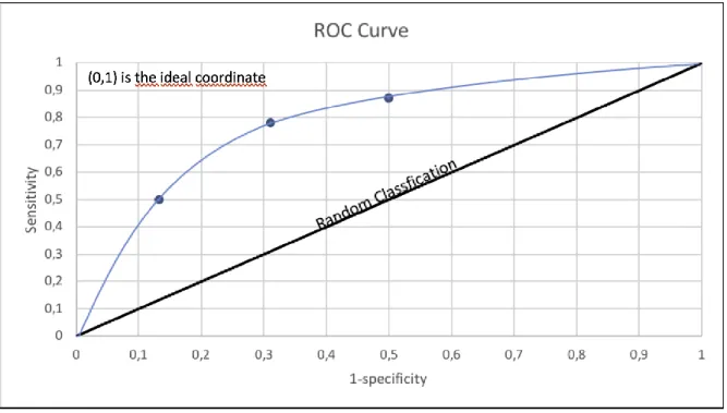
Receiver Operating Characteristic(ROC) curve is formed by plotting true positive rate in a function of false positive rate for different threshold points. True positive rate is the sensitivity represented in y-axis and the false positive rate is calculated as 1-specificity and plotted in x-axis. Each point on the ROC curve represents a sensitivity/specificity pair corresponding to a particular threshold as shown in Figure . In a test when ROC curve passes through the upper left corner then it indicates 100% sensitivity, 100% specificity. Hence a classifier with a ROC curve closer to upper left corner has a higher overall accuracy [43].
WEKA cross validation test measures the classifier’s accuracy by the area under the ROC
curve, also called AUC.
AUC is measured by using Equation 2.32.
𝐴𝑈𝐶 = ∫ 𝑅𝑂𝐶(𝑡)𝑑𝑡1
0
(2.32)
where 𝑅𝑂𝐶(𝑡) is the sensitivity and t = 1-specificity. A value of 1 is considered optimal and a
Figure 2.5:ROC Curve
2.2.4.7. Correlation coefficient
In case of predicting continuous values , correlation coefficient measures how well the predictions are correlated or change with the actual output value. It gives values between -1 and 1.A value of 0 means there is no relation and a value of 1 is a perfectly correlated set of predictions. A negative value indicates an inverse linear relation.
2.2.4.8. Mean Absolute Error(MAE)
Mean absolute error is the measure of difference between the continuous prediction and the actual data point in the data instances. The MAE is calculated as the average of absolute error per instance for all the instances in the dataset. Absolute error is the difference between the measured value and actual value(Equation 2.33).
𝑀𝐴𝐸 = ∑ |𝑃𝑟𝑒𝑑𝑖𝑐𝑡𝑒𝑑𝑖− 𝐴𝑐𝑡𝑢𝑎𝑙𝑖|
𝑁 𝑖=1
𝑁
( 2.33)
Root Mean Square Error (RMSE) is the standard deviation of the prediction errors which are a measure of how far from the regression line data points are. In other words, RMSE indicate the distribution of data around the line of best fit. RMSE metric can be calculated by Equation 2.34. 𝑅𝑀𝑆𝐸 = √∑ (𝑃𝑟𝑒𝑑𝑖𝑐𝑡𝑒𝑑𝑖− 𝐴𝑐𝑡𝑢𝑎𝑙𝑖)2 𝑁 𝑖=1 𝑁 ( 2.34)
2.3 Related studies
Considering the fact that data mining domain is flooded with algorithms and procedures, the quest for finding the perfect method has been perpetual. Several research works and case studies have led to a selection of many state-of-art algorithms which are common in use across multiple domains.
Karen Zita Haigh et al. presented a case study on the use of machine learning techniques in embedded electronics and argued the challenges faced with the usage of traditional approaches [24]. They also proposed an optimization of Super vector machine algorithm which was implemented on general purpose processors of two communications networks. Qing Chen Zhang et al. argues about the data mining challenges in IoT systems and propose two enhancement to high-order c-means algorithms for clustering big dataset and exhibit the performance improvement in terms of high compression rate without compromising with the accuracy[25]. Mark A. Hall and Geoffrey Holmes [10] benchmarked some of the attribute selection methods for supervised machine learning algorithms C4.5 and naive Bayes. They concluded that attribute selection is an effective pre-processing method to improve the mining model, along with that they also opinionated that a single method cannot be claimed as the best approach but the outcome is dependent on the model and dataset characteristics. Rafet Duriqi et al. analyses classification algorithms on three different datasets using WEKA. They picked Naive Bayes, Random Forest, and K * algorithm to perform the study and concluded that the feature count and data characteristics are influential in the performance of classifier [23].