Towards scalable Bayesian nonparametric methods for data analytics

(1)

Towards Scalable Bayesian Nonparametric Methods

for Data Analytics

by

Viet Huu Huynh,

M.Eng. (aka Huỳnh H˜_{ưu Viê.t)}

Submitted in fulfillment of the requirements for the degree of Doctor of Philosophy

Deakin University January, 2017

(2)

(3)

(4)

(5)

Acknowledgements

In many ways, I wouldn’t have been able to finish this thesis without the guidance, support, and assistance of many great people over the course of this dissertation. I would like to gratefully acknowledge the individuals and their contributions here.

First and foremost, I would like to express sincere gratitude and thanks to my principal supervisor, Prof. Dinh Phung, for his endless motivation, constant en-couragement and support. As an advisor, Dinh has enthusiasm and passion which provide driving inspiration to me, a beginning researcher, while he simultaneously allows me free rein to investigate emerging interests. I also would like to thank my co-supervisor Prof. Svetha Venkatesh for her valuable encouragement and guidance during the course of this thesis. Svetha’s scientific writing workshops greatly helped me to improve my writing and reading skills.

I, fortunately, benefited from insightful interactions and guidance from two collab-orators Dr Hung Bui and A/Prof. XuanLong Nguyen. Although geographically far away, I received great insights from discussions through video conference and email exchanges with them. I am grateful for their time, expertise and sharpness in thinking and in shaping many ideas over the course of this thesis. I am also grateful for the opportunity to interact with Dr Matthew Hoffman. His helpful discussions and valuable comments shaped the work in stochastic variational inference.

My thanks also go to all members of PRaDA for creating our workplace an encour-aging environment with many social activities after hours. Also, my special thanks go to Tu Nguyen and Thin Nguyen for kindly providing datasets which were used in Chapter 6. I also would like to thank PRaDA for providing financial support for this thesis.

I owe special thanks to my beloved wife, Hien, for her love, understanding, encour-agement, and endless support in the best and worst moments. My thanks also go to her for proofreading this thesis.

Last, but surely not least, I am infinitely indebted to my parents. Without their eternal support and encouragement, I cannot have the opportunity to freely pursue my academic interests. To them, this thesis is dedicated.

(6)

Relevant Publications

Part of this thesis and some related works have been published and documented elsewhere. The details are as follows:

Chapter 3:

• Viet Huynh, Dinh Phung, Long Nguyen, Svetha Venkatesh, Hung Bui (2015). Learning conditional latent structures from multiple data sources. In Proceed-ings of the 19th Pacific-Asia Conference on Knowledge Discovery and Data Mining (PAKDD), pp. 343-354, Vietnam. Springer-Verlag, Berlin Heidelberg.

Chapter 4:

• Viet Huynh, Dinh Phung, Svetha Venkatesh (2015). Streaming Variational Inference for Dirichlet Process Mixtures. In Proceedings of the 7th _Asian Con-ference on Machine Learning (ACML),volume 45, pages 237–252, Hong Kong.

• Viet Huynh, Dinh Phung (2017). Streaming Clustering with Bayesian Non-parametric Models. Neurocomputing (2017).

Chapter 6:

• Viet Huynh, Dinh Phung, Svetha Venkatesh, Long Nguyen, Matt Hoffman, Hung Bui (2016). Scalable Nonparametric Bayesian Multilevel Clustering. In Proceedings of the 32th Conference on Uncertainty in Artificial Intelligence, New York City, NY,USA.

(7)

List of Figures

2.1 Probabilistic graphical model classification . . . 8

2.2 A simple directed graphical model . . . 10

2.3 A simple plate graphical model . . . 11

2.4 Two statistical models are depicted as graphical models . . . 12

2.5 Undirected graphical models . . . 13

2.6 A Markov network . . . 14

2.7 A sum-product algorithm on an directed graph. . . 15

2.8 Bayesian learning process. . . 31

2.9 Conceptual level of Bayesian learning . . . 32

2.10 Bayesian Gaussian mixture models . . . 33

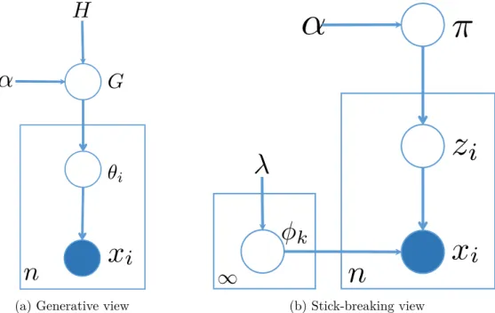
2.11 An illustration of Chinese restaurant process . . . 38

2.12 Dirichlet Process Mixture models . . . 41

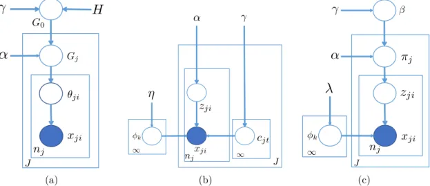
2.13 Hierarchical Dirichlet process . . . 42

2.14 Nested Dirichlet Process . . . 44

2.15 Comparing stick-breaking representation between HDP and nDP. . . 45

3.1 Graphical representation for the context sensitive Dirichlet process . . 62

3.2 Context sensitive Dirichlet process model with multiple contexts . . . 68

3.3 Results running CSDP model with RealityMining dataset . . . 71

3.4 Top 4 time topics and corresponding conditional user-IDs groups . . 72

4.1 A new representation of Dirichlet process mixture . . . 77

4.2 Steaming variational Bayesian for DPM. . . 84

4.3 Graphical presentation for DPM with product space. . . 85

4.4 Perplexity compared with baseline algorithms . . . 86

4.5 Digit clustering results with MNIST data. . . 87

4.6 Bar topics discovered by streaming algorithms . . . 88

4.7 MNIST Digit groups discovered by streaming algorithms . . . 88

4.8 Average dissimilarity between discovered topics . . . 89

4.9 Dissimilarity between topics using DPM-word model . . . 90

4.10 Dissimilarity between topics using DPM-word-author model . . . 90

4.11 Cluster proportion changed over number of mini-batches . . . 91

4.12 Topic and author groups changed in Topic 13 . . . 91

4.13 Topic and author groups changed in Topic 16 . . . 92

(13)

4.14 Predictive performance of the streaming and batch algorithms . . . . 93

5.1 Graphical representation for the HDP model. . . 100

5.2 Spark Architecture (taken from (Scott,2015)) . . . 106

5.3 A graph example in GraphX . . . 107

5.4 Three different views of a graph in GraphX API . . . 107

5.5 Data representation for topic modelling with GraphX . . . 108

5.6 Tag-clouds with MDC data . . . 113

5.7 The relationship of discovered topics and Bluetooth/WiFi IDs . . . . 115

6.1 Graphical presentation for Multilevel clustering with contexts models. 121 6.2 Variational factorization and global vs. local variables for SVI. . . 125

6.3 Perplexity with respect to running time on NIPS and NUS-WISE . . 132

A.1 Variational distribution dependency for naive mean-field. . . 143

(14)

List of Tables

2.1 Four classes of learning problems with graphical models . . . 18

3.1 Clustering performance improved when more contextual data used in the proposed model. . . 72

4.1 Notations and shortened conventions . . . 78

5.1 Data statistics . . . 110

5.2 Perplexity and running time 20 newsgroups . . . 111

5.3 Perplexity and running time for large-scale datasets . . . 112

5.4 Perplexity and running time 20 newsgroups . . . 112

6.1 Running time of two implementation versions . . . 132

6.2 Log perplexity of Wikipedia and PubMed data . . . 133

6.3 Extended Normalized mutual information (NMI) for Pubmed data . 133 6.4 Clustering performance for AUA data . . . 134

A.1 Variational parameter updates of naive and structured mean-field . . 156

A.2 Variational parameterstochasticupdates of naive and structured mean-field . . . 157

(15)

List of Algorithms

2.1 Metropolis-Hastings sampling for Bayesian inference . . . 52

2.2 Gibbs sampling for Bayesian inference . . . 54

3.1 Multiple Context CSDP Gibbs Sampler . . . 69

4.1 Truncation-free Variational Bayes for DPM . . . 82

4.2 Truncation-free Maximization Expectation for DPM . . . 82

4.3 Streaming inference for DPM . . . 84

5.1 Sparkling tCVB learning for HDP . . . 109

6.1 Stochastic variational inference for MC2 . . . 128

(16)

Abstract

I

nnovations in technology in recent decades have supplied our lives with afford-able digital devices not only for enterprises but also for personal uses. The explo-sion of digital devices has been leading to a data deluge where an immense amount of data has been continually produced at an ever increasing and extraordinary scale. This phenomenon has been widely coined as “big data”. Big data has the potential to revolutionise research, science, education, health and well-being, manufacturing, and many other disciplines in our social activities. However, data themselves – medical records, traffic patterns, enterprise content and transactions, online user-generated content such as Facebook and blog posts, tweets, online searches, signals from wearable devices, etc. – are not ready for harvesting information. Turning big data into actionable information and insights requires modelling and compu-tational techniques to reveal trends and patterns within collected datasets. When dealing with big data, there are many challenges which are broadly categorized by four dimensions (called four V’s): volume (implying enormous amounts of data), variety (referring to the multiple sources where their types are both structured and unstructured), velocity (dealing with streaming data), andveracity (referring to the uncertainty of data, e.g., with biases, noise, and abnormality). Seeking for an eleg-ant machine learning framework that can deal with these challenges is the objective of this thesis.

Bayesian analysis provides us with such an elegant framework for analysing data which has been widely embraced in AI and machine learning community. The popularity of Bayesian approaches in data analysis is due to a number of attract-ive advantages over other methods. These include natural incorporation of prior knowledge; the flexible mechanism to construct advanced models based on simple components; prevention from overfitting; handling with missing data; and explicit interpretation of uncertainties over parameters and models. Bayesian framework naturally manages veracity challenge dimension. Bayesian nonparametrics, in par-ticular, provide us even more flexible mechanism in which models can grow in size and complexity as data accumulate. They are particularly applicable to the prob-lems of big data where fixing the size of models is usually difficult, especially in streaming settings. Therefore,we ground the work of this thesis on the recent theory of Bayesian nonparametrics.

(17)

We first deal with the variety dimension of data by proposing a rich Bayesian non-parametric graphical model called context sensitive Dirichlet process model. Data usually present in heterogeneous sources. When dealing with multiple data sources, existing models often treat them independently and thus cannot explicitly model the correlation structures among data sources. To address this problem, we pro-posed a full Bayesian nonparametric approach to model correlation structures among multiple and heterogeneous datasets. The proposed framework, first, induces the mixture distribution over primary data source using hierarchical Dirichlet processes (HDP). Once conditioned on each atom (group) discovered in the previous step, context data sources are mutually independent, and each is generated from another hierarchical Dirichlet processes.

The velocity challenge in big data requires learning algorithms that can learn from a data stream. To this end, we developed a streaming clustering framework using Di-richlet process mixture (DPM) models which are the fundamental building blocks in Bayesian nonparametric modelling. Bayesian nonparametric (BNP) models are the-oretically suitable to learn streaming data due to their complexity relaxation to the volume of observed data. There are many inference algorithms for efficient learning with BNP models. However, few works leverage streaming nature of BNP to apply to real applications. In order to handle the “never-ending” nature of data in stream-ing settstream-ings, we present two variational algorithms which allow the complexity of the models to grow when necessary. One of them enables to learn fully Bayesian called TFVB (truncation-free variational Bayes) while the other supports hard clustering called TFME (truncation-free maximisation expectation). We further leverage on the works of (Broderick et al., 2013) to provide the streaming learning framework for the popular Dirichlet process mixture models.

Besides massive data stream, big data also has large (petabyte and exabyte) scales (thevolume challenge). Learning massive collections of data, which contains millions of documents or billions of data points under a Bayesian nonparametric setting, is a challenging task. The challenges come from dealing with not only big but noisy data within the complex models induced from the Bayesian formulation. While there are several efforts to design inference algorithms for latent Dirichlet allocation (LDA) in large scale settings (Liu et al., 2015; Zhai et al., 2012) which took advantage of multi-core or distributed systems, the distributed inference methods for HDP is not yet available. We then aim to fill in this gap by developing an inference algorithm for the HDP on the distributed platform Apache Spark, which allows us to handle the volume challenge of big data.

(18)

con-textual information requires a pressing need for joint modelling and, in particular, clustering the content-units (e.g., forming topics from words) and the content-groups (e.g., forming cluster of documents) — a problem known asmultilevel clustering with context (Nguyen et al., 2014) (MC2). To this end, we also address the multilevel clustering with contexts problem at scale, by developing effective posterior inference algorithms for the MC2 model using techniques from stochastic variational inference. A challenging aspect about inference for MC2 is the computational treatment in the clustering of discrete distributions of contents jointly with the context variables. Unlike either the Dirichlet process or HDP mixtures, the context-content linkage present in the MC2 model makes the model more expressive, while necessitating the inference of the joint context and content atoms. These are mathematically rich objects — while the context atoms take on usual contextual values, the con-tent atoms represent probability distributions over words. To maintain an accurate approximation of the joint context and content atoms, we employ a tree-structured mean-field decomposition that explicitly links the model context and content atoms. Similar to the work in Chapter 5, the approach can be directly parallelizable, and we provide parallelized implementations that work both on a single machine and on a distributed Apache Spark cluster.

(19)

Abbreviations

Abbreviations Meanings

i.i.d. independently and identically distributed w.r.t with respect to

BNP Bayesian nonparametrics

CRP Chinese restaurant process CRF Chinese restaurant franchise CRF-Bus Chinese restaurant franchise-bus CSDP context sensitive Dirichlet process CVB collapsed variational Bayes

DP Dirichlet process

DPM Dirichlet process mixture

DPM-PS Dirichlet process mixture with product space

ELBO Evidence Lower Bound

EMR electronic medical records GEM Griffiths-Engen-McCloskey

GMM Gaussian mixture model

EM expectation maximization

HDP Hierarchical Dirichlet process

KL Kullback-Leibler

LDA latent Dirichlet allocation MAP maximum a posteriori estimate MC2 multilevel clustering with context MCMC Markov chain Monte Carlo MLE maximum likelihood estimate

MRF Markov random field

nDP nested Dirichlet process

NMI normalized mutual information PCA principal component analysis PGM probabilistic graphical model

PPCA probabilistic principal component analysis SVI stochastic variational inference

VB variational Bayes

(20)

Chapter

1 Introduction

W

e are at the dawn of a new revolution in the Information Age: data. “Every animate and inanimate object on Earth will soon be generating data” (Smolan and Erwitt, 2013). While we collectively are tweeting 8,000 messages around the world every second, our homes, cars, cities and even our bodies are also constantly generating terabytes of signals. This phenomenon has been widely referred to as “big data” which brings the potential to revolutionise research, education, manufac-turing, health and well-being, and many other disciplines in our social activities.

However, resorting big data to actionable information involves dealing with four dimensions of challenges in big data (called four V’s): volume, variety, velocity, veracity. The volume dimension refers to a massive amount of data generated or collected by electrical devices and enterprise systems in every second. Every day we created more than 2.5 quintillion bytes data1_{. The quantity of data generated}

in recent two years accounts for approximately 90% of the data in the world. Data velocity refers to the increasing speed at which data are being generated. Social networks such as Twitter or Instagram receive more than 200,000 posts every minute. Data produced by human-being activities are usually diverse and referred as the variety characteristic. Posts in social media include different types such as texts, images, video, etc. However, the quality and accuracy of data are usually low. For example, posts on Facebook or Twitter contain hashtags, typos, or colloquial language. This property of data is mentioned as veracity.

This deluge of data requires automated algorithms for analysing. Fortunately, ma-chine learning provides a set of methods that can automatically discover hidden pat-terns in data which can be used to predict the future data or to make the decisions in some circumstances. The challenges are that these data not only present in a massive amount but also co-exist in various forms including texts, hypertext, image,

1_{A quintillion is 10}18_{, i.e., one quintillion bytes is approximately 10}9 _{GBs. These numbers are}

recorded in 2013 and growing (see infographics by Ben Walker, the marketing executive at voucher-cloud at http://www.vvoucher-cloudnews.com/wp-content/uploads/2015/04/big-data-infographic1.png).

(21)

1.1. Aims and Approaches 2

graphics, video, speech and audio from multiple channels. For example, in dealing with social network analysis, data in network connection are accompanying with users’ profiles, their comments, and activities. In medical data understanding, the patients’ information usually co-exists in various channels such as diagnosis codes, demographics, and laboratory tests. The needs for statistical modelling that can handle hidden relationships from these related data sources are inevitable. Bayesian statistical methods are increasingly popular as techniques for modelling in statist-ical and machine learning. Bayesian learning framework naturally allows us to deal veracity challenge dimension.

However, when using Bayesian parametric models for learning, we usually assume that there is a finite (and often low) number of parameters in the models. One of the limitations of parametric models is that we need to accomplish model selection for the avoidance of over-fitting and under-fitting with every new dataset. Bayesian nonparametric models, on the other hand, relax the assumption of the parameter space to be infinite-dimensional. Therefore, Bayesian nonparametric models provide a more flexible mechanism in which models can grow in size and complexity as data expand. They are particularly applicable to the problems of big data where fixing the size of models is usually difficult, especially in streaming settings. Therefore, we ground our works in this thesis on Bayesian nonparametric methodology. Regard-less of their advancement, the major burden of applying Bayesian nonparametric modelling in real-world applications is time-consuming, slow converging inference approaches for complex, high-dimensional and large-scale datasets. In this thesis, we seek for novel Bayesian nonparametric models and scalable learning algorithms which can deal with these challenges of the big data era.

1.1 Aims and Approaches

The aim of this thesis is to develop probabilistic graphical models for dealing with the big data deluge. The challenges we strive to address in this thesis include:

• To construct novel Bayesian nonparametric models for effective modelling the heterogeneity of modern datasets which are integrated from multiple sources and are highly correlated.

• To develop practicable algorithms for inference and learning Bayesian non-parametric models in big data settings in which data flow are overwhelmed and presented with noise and unreliability in some sources.

(22)

1.2. Significance and Contribution 3

Bayesian methodology provides an elegant and integrated framework to manage the uncertainty of data. Furthermore, Bayesian methods allow us to incorporate prior knowledge naturally and to construct advanced models based on simple components. Bayesian nonparametric methods, in particular, have recently emerged in machine learning and data mining as an extremely useful modelling framework due to their model flexibility capable of fitting a wide range of data types. A widely-used applica-tion of Bayesian nonparametrics is clustering data where models for inducing discrete distributions on a primary parameter space. Besides, the resilience to over-fitting of Bayesian nonparametrics makes them be the suitable framework for learning with big data. Therefore, we ground our works in this thesis on Bayesian nonparametric methodology.

There are two ways to design scalable learning algorithms for probabilistic graph-ical models which can deal with massive datasets. The first technique is to build intrinsically learning algorithms for existing models to overcome the scalability lim-itation. The second approach is to parallelize or to distribute learning algorithms to leverage multiple cores or distributed systems. For example, in the work presen-ted in Chapter 4, we used the first methodology to scale up learning algorithms by (re)designing streaming learning methods. These algorithms do not only handle “never-ending” data in streaming settings but also learn large-scale datasets. In Chapter 5 and 6, we scale up the learning algorithms by combining two techniques. First, we re-design learning algorithms for the models using the (stochastic) vari-ational inference framework, then parallelize and distribute them on Apache Spark systems. The obtained learning algorithms are several orders of magnitude faster than existing methods.

1.2 Significance and Contribution

The significance of this thesis is twofold. The first contribution is the development of Bayesian nonparametric models for learning from heterogeneous data sources while the second is to develop scalable inference algorithms for a wide range of large-scale statistical models including fundamental models. These models can be served as the building blocks to build richer models in Bayesian nonparametrics such as Dirichlet process mixture models (DPM), hierarchical Dirichlet processes (HDP) and richer models like multilevel clustering with context (MC2). Primarily, our contributions can be summarised as follows:

(23)

1.2. Significance and Contribution 4

channels in different areas of real-world applications such as pervasive comput-ing, medical data mincomput-ing, etc. We also develop a derivation of efficient parallel inference with Gibbs sampling for multiple contexts. We have further demon-strated the proposed model to discover latent activities from mobile data to answer who (co-location), when (time) and where (cell-tower ID) – a central problem in context-aware computing applications. With its expressiveness, our proposed model not only discovers latent activities (topics) of users but also reveals time and place information. Qualitatively, it is shown that better clustering performance than without them.

In seeking scalable learning algorithms that can learn modern real-world datasets containing billions of data points, our contributions are:

• Two truncation free variational algorithms for learning with Bayesian non-parametric models, particularly Dirichlet process mixture models with expo-nential family derivation solutions. Based on developed variational inference algorithms, our streaming learning algorithms can leverage on automatic “ex-panding complexity with data” nature of Bayesian nonparametric models. In addition, to cope with the availability of multiple data sources in practice, the clustering model called Dirichlet process mixtures with product space is pro-posed. We demonstrate our truncation-free algorithms with existing methods which are qualitatively comparable. We also further show the application of image and text analysis that can be learned on the fly with streaming data.

• A new inference for hierarchical Dirichlet process using collapsed variational Bayes, which is referred to as the truly collapsed variational HDP (tCVB-HDP). We further speed up the tCVB-HDP algorithm by proposing a scalable parallelized and distributed implementation on Apache Spark – a modern dis-tributed computing architecture. We have shown the improvement of proposed implementation with extensive experiments to demonstrate that the proposed algorithms outperform its parametric counterpart – LDA (which is available in Apache Spark Machine Leaning library) with a competitive running time.

• A new theoretical development of stochastic variational inference for an im-portant family of models to address the problem of multilevel clustering with contexts. We note this class of models (MC2) include nested DP (nDP), DPM, and HDP as the special cases. The approach can be directly parallelizable, and we provide parallelized implementations that work both on a single machine and on a distributed Apache Spark cluster. The experimental results demon-strate that our method is several orders of magnitude faster than existing the Gibb-sampler while yielding the same model quality. Most importantly, our

(24)

1.3. Structure of the Thesis 5

work enables the applicability of multilevel clustering to modern real-world datasets containing millions of documents.

We are going to describe these contributions in the following chapters. However, we briefly outline the content of this thesis in the following section.

1.3 Structure of the Thesis

We now provide an overview of the methods and results in the subsequent chapters. Each chapter is presented with an introductory paragraph with some detailed out-lines.

We begin this thesis by reviewing relevant literature in machine learning community upon which we develop our models and learning algorithms in Chapter 2. This chapter first describes probabilistic graphical models with three main pillars: rep-resentation, inference, and learning. Two primary representations including directed and undirected models are summarised. Exact inference and learning methods such as elimination or sum-product algorithms are also introduced. Next, we present ex-ponential families, one of the most expressive and computationally convenient classes of probability distributions, which provide a statistical representation of graphical models. We present computational details of three families (the Multinomial, Dirich-let and generalized DirichDirich-let distributions) which are extensively used in consequent chapters. Since we ground our methods in Bayesian methodology, Bayesian nonpara-metric in particular, conceptual ideas of Bayesian learning and fundamental models based on Dirichlet process, a widely used model in nonparametric Bayesian stat-istics, are also discussed. For computational issues, we conclude this chapter with two main streams of approximate inference methods for Bayesian models including variational Bayes and Markov Chain Monte Carlo (MCMC).

In Chapter 3, we propose a full Bayesian nonparametric approach to model correl-ation structures among multiple and heterogeneous datasets. The proposed model induces mixture distribution over primary data source using hierarchical Dirichlet processes (HDP). Once conditioned on each atom (group) discovered in the previous step, context data sources are mutually independent. Each context data is gener-ated from hierarchical Dirichlet processes. In each particular application, which covariates constitute content or context(s) is determined by the nature of data. We demonstrate our model to address the problem of latent activities discovery in pervasive computing using mobile data. We show the advantage of utilising

(25)

mul-1.3. Structure of the Thesis 6

tiple data sources regarding exploratory analysis as well as quantitative clustering performance.

The second half of this thesis focuses on the development of learning methods that can deal with streaming and high volume data. In Chapter 4, we aim to address the challenges of learning from data stream without the need to revisit the past data. In order to handle with “never-ending” data in streaming settings, we present two variational algorithms which allow model complexity to grow automatically when necessary. We first introduce two truncation-free variational inference algorithms which do not need to fix the size of models. We further develop streaming learning framework for the popular Dirichlet process mixture (DPM) and Dirichlet process mixture with product space (of data channels) (DPM-PS). The latter allows us to learn data from multiple data sources. Evaluation of streaming learning algorithms with text corpora reveals both quantitative and qualitative efficacy of the algorithms on clustering documents.

Chapter 5 scales up hierarchical clustering for large datasets. This chapter strives to design learning algorithms for hierarchical clustering problems, e.g. topic model-ling with massive collections with the total number of data points up to billions. We develop a novel collapsed variational Bayes inference for HDP in which we collapsed the stick-breaking variables and global topics without introducing any auxiliary variables. We call the algorithm as truly collapsed variational Bayes (tCVB). We further improve the scalability of truly collapsed variational Bayes by deploying on distributed systems Apache Spark. Consequently, it usually takes days (to weeks) to learn the large corpora with a single machine, we can learn the same data with the distributed learning algorithms for hours.

A limitation of current nonparametric Bayesian models is its ability to deal with un-structured data where meta–data exists at multiple levels such as the document or group-specific information. This is largely due to the expensive computation when more sophisticated model choices are made. In Chapter 6, we aim to address the multilevel clustering with contexts problem at scale, by developing effective pos-terior inference algorithms for the MC2 using techniques from stochastic variational inference. We yield another speeding up level with a scalable implementation of the proposed SVI-MC2 on Apache Spark. We have illustrated that our new algorithm can scale up to very large corpora.

Finally, we conclude this thesis with remarks on contributions of the thesis and discuss potential avenues for future research in Chapter 7.

(26)

Chapter

2 Related Background

T

he work of this dissertation has its root in a statistical approach to machine learning. In particular, it builds upon the foundation of probabilistic graphic models. Probabilistic graphical models offer a unified framework for constructing large-scale statistical models and capturing the uncertainty. In the first part of this chapter, we review elements of graphical models including graphical representations, inference and learning methods. We then describe exponential families of probability distributions, also known as log-linear models, which could, in most cases, provide the alternative distributional view for graphical models. Exponential families can be also considered as the solutions to maximum entropy problems and possess several important properties that facilitate tractability and computational conveniences. The area of Bayesian learning will then be briefly introduced with an emphasis on the context of the exponential family. Finally, we conclude this chapter with an introduction to two major approaches for approximate inference the graphical models: variational inference and Markov Chain Monte Carlo (MCMC).

2.1 Probabilistic Graphical Models

Probabilistic graphical models1 ₍_Pearl_,₁₉₈₈_; _Lauritzen_, ₁₉₉₆_; _Jordan_,₂₀₀₄_{), which}

combine probability theory and graph theory, provide an elegant framework for en-coding uncertainty and structured complexity occurring throughout the complex, real-world phenomena. The graph-base theory of graphical models provides intu-itively appealing compound to compactly represent complex interactions of large sets of random variables while the probability-theoretic side contributes means to integrate models to data. The probabilistic aspect of graphical models also provides mechanisms to stick the components in models into a consistent system. The be-nefits of graphical models as modelling tools can be concisely summarised in the

1_{In this thesis, we use the terms “probabilistic graphical model(s)” and “graphical model(s)”}

interchangeably.

(27)

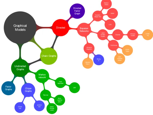
2.1. Probabilistic Graphical Models 8 Graphical Models Directed Directed Factor Graph Bayesian Networks Dynamic Bayes nets Markov chains HMM LDS Latent variable models Discrete Mixture models cluster-ing Continuous dimen-reduct over-complete repres. Inﬂuence diagrams Strong JT Decision theory Chain Graphs Undirected Graphs Markov network input dependent CRF Pairwise Boltz. machine Pdisc.z Gauss. Process Pcontz Clique Graphs Junction tree Clique tree Factor Graphs

Figure 2.1: Probabilistic graphical model classification, courtesy of David Barber (Barber, 2012)

Preface of (Jordan, 1998).

“Many of the classical multivariate probabilistic systems studied in fields such as statistics, systems engineering, information theory, pattern re-cognition and statistical mechanics are special cases of the general graph-ical model formalism – examples include mixture models, factor analysis, hidden Markov models, Kalman filters and Ising models. The graphical model framework provides a way to view all of these systems as instances of a common underlying formalism. This view has many advantages – in particular, specialized techniques that have been developed in one field can be transferred between research communities and exploited more widely. Moreover, the graphical model formalism provides a natural framework for the design of new systems.”

A probabilistic graphical model (PGM) is a graph where each node represents a random variable while an edge between two vertices denotes the (conditional) de-pendence assumptions between the corresponding nodes. At a high level, a graphical model with n nodes introduces a joint probability distribution over some collection

(28)

2.1. Probabilistic Graphical Models 9

of random variables X _,{X1, . . . , Xn}. For instance, if these variables are binary, we need O(2n) parameters to capture the joint distribution. However, depending on the conditional assumptions encoded by the structure of the graph, the graphical model endowed with this collection of random variables will reduce the required parameters exponentially. The independence properties in the joint distribution that the graphical model exploits as structural characteristic existing in many real-world applications. Therefore, graphical models provide a fruitful mechanism for characterising large-scale multivariate statistical models.

In graphical models, the two most popular classes, which are classified based on graphs forms, aredirected (acyclic) graphical modelsandundirected graphical models. The former is also known as Bayesian networks, belief networks, generative models, causal models, etc. in the context of the AI and machine learning communities (Pearl, 1988) while the latter is usually referred to as Markov networks or Markov random fields in the literature of the physics and computer vision communities. However, the categorization does not confine in that border. Though less popular, there is also the work on chain graphs (Buntine, 1995; Lauritzen, 1996), hybrid or mixed directed and undirected representations. Hierarchy for graphical model classification is presented in Figure 2.1, borrowed from (Barber, 2012). A more detailed discussion of these models can be found in the comprehensive book by (Barber, 2012). In this section, we briefly review different aspects of graphical models including representation, inference and learning.

2.1.1 Representation

Directed graphical models also known as Bayesian networks are directed acyclic graphs (DAG) G(V, E), where V ={x1, . . . , xn} are n random variable nodes, and E are the directional edges. An edge from a node A to a nodeB can be informally interpreted as the “influence” ofAtoB. Each random variable or node in the graph has a corresponding(conditional) probability distribution,p(xi |πxi), whereπxiis the

collection of parental nodes ofxi. Note that the(conditional) probability distribution p(xi |πxi) can be discrete or continuous. The joint probability distribution can be

factorised according to graph G into a product p(x1:n) =

n

Y

i=1

p(xi |πxi), (2.1)

where again πxi are parental nodes of xi. The factorization in Equation (2.1) is

ob-tained by the conditional independence assumptions in a Bayesian network. These are also called local Markov assumptions which state informally that a node is inde-pendent of its ancestors given its parents. There is a one-to-one mapping between

(29)

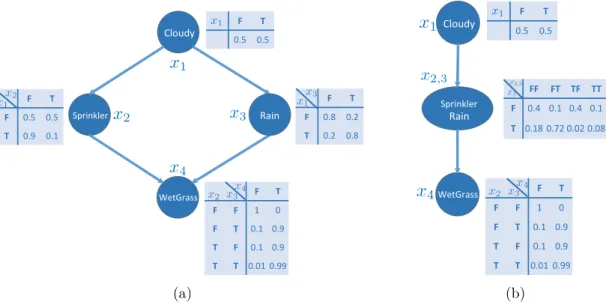
2.1. Probabilistic Graphical Models 10 F T F 0.5 0.5 T 0.9 0.1 F T F 0.8 0.2 T 0.2 0.8 F T 0.5 0.5 F T F F 1 0 F T 0.1 0.9 T F 0.1 0.9 T T 0.01 0.99 Cloudy Sprinkler WetGrass Rain (a) FF FT TF TT F _{0.4 0.1 0.4 0.1} T _{0.18 0.72 0.02 0.08} F T 0.5 0.5 F T F F 1 0 F T 0.1 0.9 T F _0.1 _0.9 T T _{0.01 0.99} Cloudy WetGrass Sprinkler Rain (b)

Figure 2.2: A simple directed graphical model (a.k.a. Bayesian network), adapted from (Russell and Norvig, 2009). Each table associated with each node specifies a conditional probability distribution.

local Markov assumptions in graph G and factorization of the joint probability dis-tribution2_.

The conditional independence relationships in a Bayesian network allow us to rep-resent the joint distribution more compactly as we demonstrate in a simple example with the network in Figure2.2which includes four binary random variables. Without specifying any dependence structure on these variables, the full joint probability re-quires O(2n_{) parameters. However, given the graph structure in Figure} _2.2_{, the} joint distribution is now simplified to

p(x1, x2, x3, x4) = p(x4 |x2, x3)p(x2 |x1)p(x3 |x1)p(x1).

The factorization in above equation can be viewed as a result of the chain rule of probability

p(x1, x2, x3, x4) = p(x4 |x2, x3, x1)p(x2 |x1, x3)p(x3 |x1)p(x1),

which is then simplified with the dependency encoded in Figure 2.2. The number of parameters to characterize the distribution now is O(23).

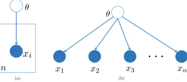
When working with a problem with a large number of random variables, many of which are replicated and appeared in nested structures, a plate notation can be a useful tool to capture replication and reduce the clutter of graphical models. A simple graphical model with plate notation is depicted in Figure2.3awhich is neater than its equivalent full representation in Figure 2.3b.

(30)

(a) (b)

Figure 2.3: A simple plate graphical model and its equivalent representation.

Examples. Many statistical models which are powerful methods in data analysis and statistics can be represented under the umbrella of directed graphical models. We illustrate two popular models which now can be interpreted in the language of graphical models including factor analysis (and principle component analysis), and Gaussian mixture model. The former is a ubiquitous technique for dimensionality reduction while the latter is a powerful tool for density estimation in statistics and clustering in machine learning.

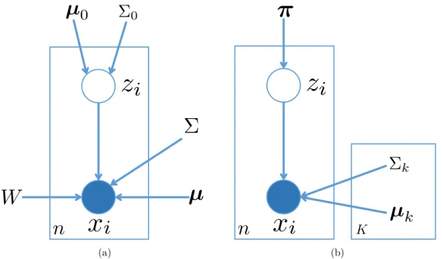
Classical PCA (principle component analysis) is a well-established technique for dealing with high-dimensional data in machine learning which projects observed data vectors (of d dimensions) into a lower dimensional vector space (q dimensions, q < d) so that the projected data are with the maximised variances. However, classical PCA is sensitive to noise and outlying observations. Probabilistic PCA (PPCA) can address these limitations. In Figure 2.4a, we illustrate the graphical model for a broader class of model called factor analysis which includes PPCA.

The graphical model itself does not provide enough information to describe mod-elling assumption. Therefore, a generative description is usually associated with a model. The generative procedure for the model in Figure 2.4ais as follows: the lat-ent variable zi with dimension q follows a multivariate Gaussian distribution, zi ∼

N (µ₀,Σ0) whereµ0 and Σ0 are mean and covariance matrix. The observation data

xi is generated from a conditional multivariate Gaussian, xi |zi ∼ N(Wzi +µ,Σ). Note thatW is ad×qmatrix called weight matrix and µis ad-dimensional vector.

Probabilistic PCA is a special case of factor analysis model wherein the noise cov-ariance matrix Σ is isotropic, i.e., Σ =σI. Classical PCAcan be obtained by taking the σ→0 limit.

(31)

(a) (b)

Figure 2.4: Two statistical models are depicted as graphical models: (a) factor analysis model which generalizes a well-known dimension reduction methods, prin-ciple component analysis (PCA); (b) Gaussian mixture model with latent indicator variables.

Another popular model in statistics and machine learning isGaussian mixture model which mixes several Gaussian components with appropriate mixing proportions. The probability distribution for this mixture is

p(x|Θ) = K X k=1 πkN (x|µ_k,Σk), where PK

k=1πk = 1. Working directly with the above mixture description might be difficult for learning. This specification be equivalently viewed as a graphical model by augmenting the mixture distribution with indicator variables, zi’s, which define the Gaussian component the data pointxi’s belong to. The graphical model for this distribution is summarised in Figure 2.4b which now has the following generative process zi ∼Cat (π), xi ∼ N µ_z_i,Σzi , (2.2)

where Cat (π) denotes a Categorical distribution with parameter vector π, while

N (µ,Σ) represents a Gaussian distribution with mean µand covariance matrix Σ. There are K Gaussian components in the model. The indicator variable zi defines the component data point xi generated from. Therefore, we can use zi as the index for the component as in Equation (2.2).

Undirected graphical models are the second most popular class of probabilistic graphical models which are also known asMarkov networksorMarkov random fields.

(32)

(a) (b)

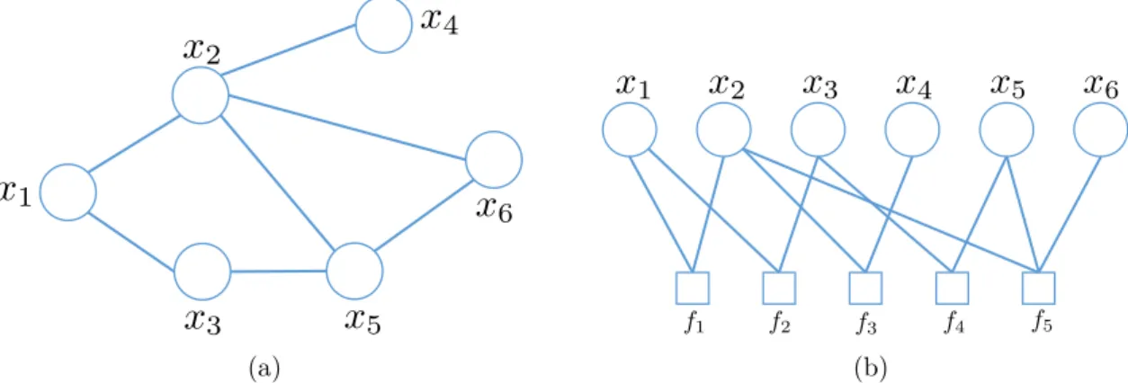
Figure 2.5: Undirected graphical models: (a) A simple undirected graphical model with 6 random variables, adapted from(Jordan, 2004); (b) its equivalent factor graph.

A undirected graph G(V, E), whereV ={x1, . . . , xn}, includes a collection of (max-imal) cliques3 _C _{of the graph. Each clique} _c_{∈ C} _{is associated with a non-negative}

functionψc(xc) called apotential function. The joint probability distributionp(x1:n) is now defined as the normalised product of the potential functions represented in the graph as p(x1:n) = 1 Z Y c∈C ψ(xc), (2.3)

where Z is a normalisation factor to keep p(x1:n) as a proper probability distribu-tion. Similar to directed graphical models, Hammersley-Clifford theorem asserts the unique mapping between graph G and product of factors based on maximal cliques of the graph under some conditions (cf.Koller and Friedman,2009, Theorem 19.3.1). Figure2.5aillustrates a simple undirected graphical model with six random variables and five potential functions. This defines a joint distribution as follows

p(x1:6) =

1

Zψ(x1, x2)ψ(x1, x3)ψ(x3, x5)ψ(x2, x4)ψ(x2, x5, x6), where the normalised factor

Z =X x1:6

ψ(x1, x2)ψ(x1, x3)ψ(x3, x5)ψ(x2, x4)ψ(x2, x5, x6).

It is convenient to use an equal representation known as a factor graph ( Kschis-chang et al., 2001) to handle graphical models including cliques with high-order potentials. Factor graphs are undirected bipartite graphs with two groups of nodes. The round nodes represent random variables similar to those in undirected or direc-ted graphs while the square nodes depict factors. Each arc between a variable and a factor denotes the occurrence of that variable in the factor. A more fine-grained

(33)

Figure 2.6: A simple undirected graphical model a.k.a. Markov network or Markov random field, a common model in computer vision. The shaded nodes, x1, . . . , x4

are observations which may correspond to pixels (or super-pixels) of an image, while the hidden nodes z1, . . . , z4 are appropriate latent labels.

representation of factor graphs is convenient to exploit the structure of the graph in developing inference algorithms. The factor graph in Figure 2.5b equivalently represents the Markov network in Figure 2.5a. The factors f1, . . . , f4 correspond

to potentials ψ(x1, x2), . . . , ψ(x2, x4) while the factor f5 involving three variables

x2, x5, x6 represents the potential ψ(x2, x5, x6).

Example. Let us consider a pixel labelling problem which aims to classify the class label of each pixel from a pre-defined set of labels. The graphical model in Figure 2.6 defines a structure for learning the pixel label of images. This model is also called pairwise conditional Markov random fields where the pixel observations x1:4

are independent when conditioning on their labelsz1:4 (Bishop,2006). However, the

model also captures the smoothness nature of images in which neighbour pixels tend to share the labels, pairwise potentials between two adjacent pixels are defined. This principle of constructing models is popular for learning computer vision problems.

2.1.2 Inference and Learning

Graphical models provide an elegant framework to deal with uncertainty in many real-world applications. Based on the graphical representation, we can represent, learn, and infer information and knowledge from the available data. These activities involve two main types of algorithms: inference and learning. The main objective of inference is to answer a query of variables of interest given certain evidences provided for the remaining set of variables and the model parameters. There are

(34)

(a) (b)

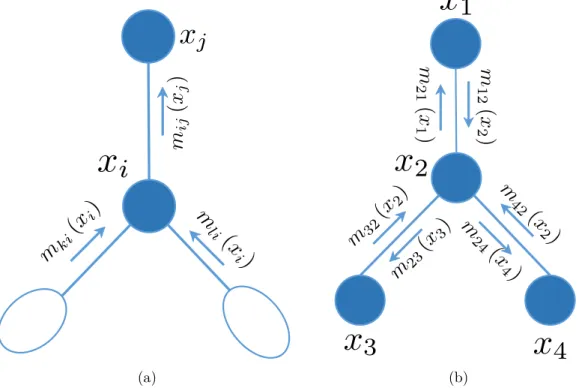
Figure 2.7: Messages when running sum-product algorithm on an directed graph, adapted from(Jordan, 2004): (a) Messages generated by the elimination algorithm, message mji(xi) from node j to node i is obtained when all of its children nodes (node k and l) eliminated and their messages (mki(xi) and mli(xi)) obtained (b) The equivalent factor graph for undirected graphical model is on the left.

many forms of queries on the models such as conditional queries, marginal queries. However, from the computational point of view, it suffices to focus on the problem of marginalisation since a conditional query p(X |E=e) can be computed using two marginal probabilities p(X |E=e) = p(_pX₍_e,e₎). Learning task usually refers to the situation that we do not know the structure (dependencies between variables), or the parameters of random variables, or both. In the following section, we describe specific problems related toinferenceandlearning commonly encountered in working graphical models.

Before discussing on specific inference algorithms, it is essential to note that directed graphical models can be converted to undirected graphical models4_{. This can be}

performed via a procedure known as moralization as follows (Jordan,2003; Bishop,

2006). All parents of the same nodes must be joined and then all directed links are dropped to become undirected. Each conditional probability p(xi |πxi) now

becomes the potential of clique ci ={xi, πxi}. Thus we can exclusively work within

the undirected framework.

(35)

Inference. We briefly outline three prominent classes of algorithms that seek the solutions for the inference problems, including exact methods, simulating methods, variational algorithms. For the comprehensive presentation, one may refer to (Koller and Friedman, 2009;Wainwright and Jordan, 2008; Andrieu et al.,2003).

Exact algorithms. Let us consider the graphical model given in Figure 2.2 and suppose that we would like to compute the marginal probability for wet grass which can be obtained by summing over other variables:

p(x4) =

X

x1,x2,x3

p(x1, x2, x3, x4).

We can naively compute the above probability by summing all possible values of remaining variables with a computational complexity of O(24_{). However, this will}

grow exponentially and an important ingredient of graphical model theory is to reduce the complexity by exploiting independent structure in the graphical model as follows p(x4) = X x1 p(x1) X x2 p(x2 |x1) X x3 p(x3 |x1)p(x4 |x2, x3) =X x1 p(x1) X x2 p(x2 |x1)m3(x1, x2, x4) =X x1 p(x1)m2(x1, x4) =m1(x4).

where mi denotes intermediate marginal distribution in which xi was marginalised. The complexity of the new computation strategy is reduced to O(23_{) since each}

term involving at most three variables. With more complex graphical models with sparse dependency, the computational complexity can be scaled down significantly.

The technique used in the previous example is known as variable elimination. We can choose different orders of elimination which will lead to different complexities. The problems of choosing the elimination order that give the least computational cost can beN P-hard (Arnborget al.,1987). One limitation of the basic elimination methodology is the restriction to a single marginal probability. If we wish to avoid redundant computation when aiming to compute several marginals at the same time, the sum-product algorithm (or belief propagation) can provide a solution for such problems. We can consider the sum-product algorithm as a dynamic programming algorithm for computing multiple marginals. Note that the sum-product method is designed to work only on (directed or undirected) trees (Wainwright and Jordan,

2008).

The sum-product algorithm is constructed by leveraging the recursive structure of a tree and using two main operators calledgenerating messages with node elimination

(36)

and aggregating messages from neighbours. In the elimination steps, we choose the order in which all children of a node will be eliminated before that node is removed. The messages obtained through elimination can be written in the following (see Figure 2.7a) mij(xj) = X xi  ψ(xi)ψ(xi, xj) Y k∈N(i)\j mki(xi)  , (2.4)

where mji(xi) denotes the message passing from node j to node i and xi as the received node; N(i) is the set of neighbours of node i. The marginal of desired node q can be computed by aggregating messages from its neighbours

p(xq)∝ψ(xq)

Y

e∈N(q)

meq(xq).

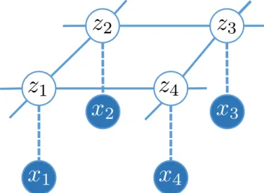
Let us consider an example of graph with four nodes in Figure 2.7b. If we want to compute the marginals of all nodes in the graphs, we need to “pass” messages to all nodes using elimination algorithm to obtain the message in Equation (2.4). In total, we will need to compute 6 messages. In a general case, it can be shown that we need to calculate all of the 2E possible messages whereE is the number of edges.

If our graphical models have loops or cycles as shown in Figure 2.2 (after moraliza-tion), we can convert the graphical model into a tree, by clustering nodes together as in Figure 2.2b. The obtained tree now contains nodes as cliques. The message passing scheme can be applied to do inference on graphs. One of the most common algorithms is called the junction tree algorithm (see (Jordan, 2003, Chapter 17), (Koller and Friedman, 2009, Chapter 11), and (Barber, 2012, Chapter 6) for the detailed presentation).

When working with complex graphical models, the running time of exact algorithms usually increases exponentially with the induced width of the graph. Furthermore, if some of the nodes are continuous random variables, the integrals of these vari-ables usually cannot be obtained in closed form. Therefore, approximate inference provides a tractable solution for inference problems on graphical models. There are two popular groups of approximate inference methods: sampling algorithms and variational algorithms. In this section, we provide a brief summary of these methods. We will elaborate on these methods with more details in Section 2.4.

Sampling algorithms provide a general methodology for probabilistic inference (Robert and Casella, 2005). The central idea of sampling-based methods is to evaluate the quantity of interest by sampling corresponding probability distributions which are computationally intractable. To sample from standard distributions, e.g. Uniform, Beta, etc., inverse and transformation methods can be used, while rejection or im-portance sampling methods allow us to sample from more complicated distributions.

(37)

However, these methods suffer from high dimensionality of data which can be over-come with a class of method called Markov Chain Monte Carlo (MCMC) including the Metropolis-Hastings algorithms and Gibbs sampling as special cases. The com-prehensive exposition of these methods might be found in numerous textbooks and papers such as (Andrieuet al., 2003; Robert and Casella, 2005; Neal, 1993).

Variational algorithms, on the other hand, are another approximate inference meth-ods based on the basic idea of casting a problem of computing probability distribu-tion to an optimizadistribu-tion problem. The optimizadistribu-tion problem is typically formed to minimise the Kullback-Leibler (KL) divergence between proxy (approximate) distri-bution and target (true) distridistri-bution. The simplest of the approximate distridistri-bution is the mean-field approximation which decouples all the nodes (removing the edges). The mean-field approximation introduces a lower bound on the likelihood which we try to maximise. In this thesis we mainly ground our inference methods on this variational framework. Hence we will develop the detailed presentation in Section 2.4 with complementary recommended readings include (Wainwright and Jordan,

2008; Jaakkola, 2000; Beal,2003)

Learning. While the main goal of inference problems is to infer the marginal or conditional probability for a known structure and known joint distribution graphical model, the goal of learning is to construct the distributions of random variables and the dependency structure between them. Depending on the availability of observa-tions and dependency structure, we can have four classes of learning problems in Table 2.1.

Structure Observability

Full Partial

Known Parameters Parameters and Hidden Nodes

Unknown Parameters and Structure Parameters, Hidden Nodes, and Structure Table 2.1: Four classes of learning problems with graphical models. Given observed data, we need to learn three elements: parameters, hidden nodes, and structure. The elements to be learned depend on the availability of structure and observability data.

When the structure is known, the main objective of learning becomes a parameter estimation problem which essentially exploits the inference algorithms described earlier. The main algorithms to learn parameters include maximum likelihood es-timates (MLE) or maximum a posteriori eses-timates (MAP) when the data are fully observed or the Expectation Maximization (EM) when there are latent variables (Murphy,2012;Koller and Friedman,2009). On the other hand, when the structure

(38)

2.2. Exponential Family 19

is unknown, it becomes a structure learning problem which is much harder to solve. The key idea is to learn (iteratively) the structure then to learn the parameters. When the structure is defined, the learning problem becomes a known structure.

Let us consider the case when the structure isunknown, but the data isfully observed. One can consider a fully connected graph, but this will introduce an overwhelming number of parameters. Another solution is to search for the highest scoring graph where the scoring function is defined to maximise the posterior of the graph given data (Murphy,2001). The hardest case of all is when the structure is unknown, and part of nodes are unobserved. There are a limit number of researches addressing these challenges. One possible approach is first to use Laplace approximation to learn the parameter of hidden variables which now turn the problem to the unknown structure and fully observed (Heckerman, 2008; Chickering and Heckerman, 1997). In this thesis, we only work with the parameter estimation problems where the structure is known in advance.

2.2 Exponential Family

In this section we summarise exponential families, a broad class of probability distri-butions which are popular in statistics and machine learning literature. Furthermore, they are closely related to graphical models in which many popular models can be represented through exponential families.

2.2.1 Exponential Family of Distributions

Definition and properties. Let x be a random variable taking value in the domain X and T be a vector-valued function T : X → _Rd _{so that} _T₍_x_{) is} d-dimensional vector. Letθ, also in_Rd_{, denote the parameter. We represent the inner} product between two vectors x,y in _Rd _by _h_x_,_y_i ₌ _xT_y_{. The probability density} for exponential family with respect to base measure µis defined as

p(x|θ) = exp{hθ, T(x)i −A(θ)}, (2.5) where A(θ) is simply a normalization term to makeP(x|θ) sums up to one and

A(θ) = ln (ˆ X exp (hθ, T(x)i)dµ(x) ) .

The entity A(θ) is called log-partition function or cumulant function while the vector T (x) is usually referred to asfeature function or sufficient statistics. When

(39)

2.2. Exponential Family 20

normalization constant A(θ) can be ignored, one can write

p(x|θ)∝exp{hθ, T(x)i}.

So far, we have conveniently ignored the constraints on θ so that A(θ) does not diverge, that is ´_Xexp (hθ, T(x)i)dµ(x) < ∞. While this is always true for finite discrete random variable x, care needs to be taken if the domain X is continuous, or discrete but infinitely countable. In the general case, the parameter θ should be viewed as restricted to the set Θ =nθ ∈_Rd _|´

X exp (hθ, T (x)i)dµ(x)<∞

o

.

Remark. In some settings, it is convenient to define a base function h : X → _R+

which is induced from base measure µ(x) and defined

p(x|θ) = h(x) exp{hθ, T(x)i −A(θ)}. (2.6)

In most cases, adding the termh(x) does not change the nature of the problem that we are dealing with. We thus assume h(x) = 1 in most of the following discussion, and will explicitly call out h(x) when we need to.

The log-partition function plays an important role while learning with exponential families. We now look a deeper exploration of the properties of this function. One of the most important properties of function Ais theconvexity which states that its first and second order partial derivatives are the expectation and covariance matrix of the feature vector, respectively

∂A(θ)

∂θ =E[T(x)]p(x|θ), and

∂2_A₍_θ₎

∂θ∂θ> = Cov [T (x)]p(x|θ). (2.7)

Since the covariance matrix is always semi-definite, i.e., ∂_∂2_θA_∂(_θθ>) 0, the log partition

function A(θ) is convex. Furthermore, the partial derivatives of the likelihood and the log-likelihood also have the closed form, involving the difference between the empirical feature vector, (T (x)), and its expectation, _E[T(x)]_p₍_x_|_θ₎.