Hypergraph Partitioning in the Cloud

(1)

Durham E-Theses

Hypergraph Partitioning in the Cloud

LOTFIFAR, FOAD

How to cite:

LOTFIFAR, FOAD (2016) Hypergraph Partitioning in the Cloud, Durham theses, Durham University. Available at Durham E-Theses Online: http://etheses.dur.ac.uk/11529/

Use policy

The full-text may be used and/or reproduced, and given to third parties in any format or medium, without prior permission or charge, for personal research or study, educational, or not-for-prot purposes provided that:

• a full bibliographic reference is made to the original source • alinkis made to the metadata record in Durham E-Theses • the full-text is not changed in any way

The full-text must not be sold in any format or medium without the formal permission of the copyright holders. Please consult thefull Durham E-Theses policyfor further details.

Academic Support Oce, Durham University, University Oce, Old Elvet, Durham DH1 3HP e-mail: [email protected] Tel: +44 0191 334 6107

(2)

Hypergraph Partitioning in the Cloud

Foad Lotfifar

Abstract

The thesis investigates the partitioning and load balancing problem which has many applications in High Performance Computing (HPC). The application to be partitioned is described with a graph or hypergraph. The latter is of greater interest as hypergraphs, compared to graphs, have a more general structure and can be used to model more complex relationships between groups of objects such as non-symmetric dependencies. Optimal graph and hypergraph partitioning is known to be NP-Hard but good polynomial time heuristic algorithms have been proposed.

In this thesis, we propose two multi-level hypergraph partitioning algorithms. The algorithms are based on rough set clustering techniques. The first algorithm, which is a serial algorithm, obtains high quality partitionings and improves the partitioning cut by up to 71% compared to the state-of-the-art serial hypergraph partitioning algorithms. Furthermore, the capacity of serial algorithms is limited due to the rapid growth of problem sizes of distributed applications. Consequently, we also propose a parallel hypergraph partitioning algorithm. Considering the generality of the hypergraph model, designing a parallel algorithm is difficult and the available parallel hypergraph algorithms offer less scalability compared to their graph counterparts. The issue is twofold: the parallel algorithm and the complexity of the hypergraph structure. Our parallel algorithm provides a trade-off between global and local vertex clustering decisions. By employing novel techniques and approaches, our algorithm achieves better scalability than the state-of-the-art parallel hypergraph partitioner in theZoltan tool on a set of benchmarks, especially ones with irregular structure.

Furthermore, recent advances in cloud computing and the services they provide have led to a trend in moving HPC and large scale distributed applications into the cloud. Despite its advantages, some aspects of the cloud, such as limited network resources, present a challenge to running communication-intensive applications and

(3)

i

make them non-scalable in the cloud. While hypergraph partitioning is proposed as a solution for decreasing the communication overhead within parallel distributed applications, it can also offer advantages for running these applications in the cloud. The partitioning is usually done as a pre-processing step before running the parallel application. As parallel hypergraph partitioning itself is a communication-intensive operation, running it in the cloud is hard and suffers from poor scalability. The thesis also investigates the scalability of parallel hypergraph partitioning algorithms in the cloud, the challenges they present, and proposes solutions to improve the cost/performance ratio for running the partitioning problem in the cloud.

Our algorithms are implemented as a new hypergraph partitioning package within

Zoltan. It is an open source Linux-based toolkit for parallel partitioning, load balancing and data-management designed at Sandia National Labs. The algorithms are known asFEHG and PFEHG algorithms.

(4)

Hypergraph Partitioning in the

Cloud

Foad Lotfifar

A Thesis presented for the degree of

Doctor of Philosophy

Algorithms and Complexity Group

School of Engineering and Computing Sciences

University of Durham

United Kingdom

(5)

Contents v 6 Conclusions 190 6.1 Summary of Achievements . . . 190 6.2 Future Work . . . 194 Appendix 197 A Benchmark Specification 197 B Programming Interface 202 B.1 Introduction . . . 202 B.2 Zoltan at a Glance . . . 203 B.2.1 General Functions . . . 206 B.2.2 Query Functions . . . 208 B.2.3 General Parameters . . . 218

B.3 FEHG Algorithm Parameters . . . 220

B.3.1 Partitioning Parameters . . . 220

B.3.2 Coarsening Parameters . . . 221

B.3.3 Initial Partitioning Parameters . . . 226

B.3.4 Uncoarsening Parameters . . . 226

B.3.5 Recursive Bipartitioning Parameters . . . 227

(8)

List of Figures

2.1 A sample hypergraph (left) with its incidence (middle) and adjacency (right) matrices. . . 16 2.2 The general reference model of the cloud. . . 26 2.3 Infrastructure-as-a-Service (IaaS) architecture and its components

[BVS13]. . . 29 2.4 Storage hierarchy in a distributed storage datacenter from

program-mers point of view [BCH13]. . . 31 2.5 Latency, bandwidth and capacity of storage access in the storage

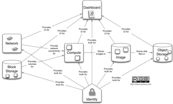
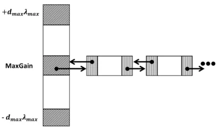
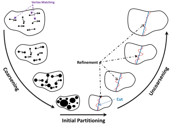
hierarchy of a distributed storage datacenter [BCH13]. . . 32 2.6 Architecture of the OpenStack cloud software. . . 34 3.1 Gain bucket data structure in Fidduccia-Mattheyses (FM) algorithm. 44 3.2 The multi-level hypergrapph bipartitioning paradigm and its three

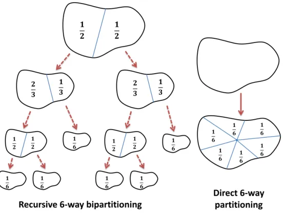
phases: coarsening, initial partitioning, and uncoarsening. . . 53 3.3 Recursive 6-way bipartitioning of the hypergraph vs direct 6-way

partitioning . . . 62 3.4 An example of a conflict that happens in the parallel FM refinement

algorithm when processors decide about vertex moves independently. Processor p1 and p2 move v1 and v2 to the other part, respectively.

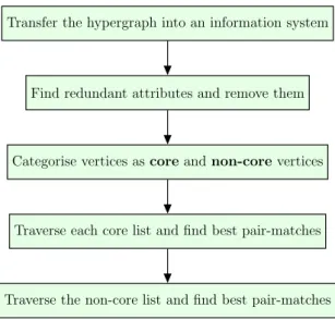
This increases the cost of partitioning from 4 to 9. The red line shows the boundary between two processors. . . 71 4.1 The coarsening phase at a glance. The non-core vertex list is processed

after all core vertices have been processed. . . 100

(9)

List of Figures vii

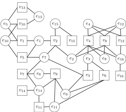
4.2 A sample hypergraph with 16 vertices and hyperedges. Vertices and hyperedges are represented as square and circular nodes, respectively. The weight of the vertices and hyperedges are assumed to be unit. . 101 4.3 An example of Hyperedge Connectivity Graph (HCG) of the

hyper-graph depicted in Fig. 4.2. The similarity threshold is s= 0.5. . . 104 4.4 The variation of bipartitioning cut based on the clustering threshold

for some of the tested hypergraphs. Values are normalised with the best cut for each hypergraph. . . 111 4.5 Comparing the cut variation for different partitioning numbers. The

weight of vertices are unit and the weight of hyperedges are their sizes.120 4.5 (Continued) Comparing the cut variation for different partitioning

numbers. The weight of vertices are unit and the weight of hyperedges are their sizes. . . 121 4.5 (Continued) Comparing the cut variation for different partitioning

numbers. The weight of vertices are unit and the weight of hyperedges are their sizes. . . 122 4.5 (Continued) Comparing the cut variation for different partitioning

numbers. The weight of vertices are unit and the weight of hyperedges are their sizes. . . 123 5.1 An example of the first round of parallel HCG algorithm. . . 134 5.2 The two rounds of parallel HCG example in Fig. 5.1. Dashed, solid, and

red lines show network communications, stabilised X to Y partitions, and representative dependency inY, respectively. The algorithm stops after two rounds. . . 135 5.3 An example of the matching algorithm. The similarity threshold is

set to s= 0.5. Vertices are categorised into cores according to edge partitions EPi and rough set clustering definitions. . . 137

5.4 The variation of bipartitioning cut in different levels of uncoarsening. The values are normalised in [0,1] based on the minimum and the maximum cut. . . 143

(10)

List of Figures viii

5.5 The percentage of the locked hyperedges in different levels of uncoars-ening. The values are the average values over all passes of the FM algorithm in each coarsening level. . . 144 5.6 The cut reduction of our FM algorithm for a bipartitioning on

CNR-2000 with variable number of processors. . . 153 5.7 The running time of the FM algorithm on different number of

proces-sors for a bipartitioning of the hypergraphs. Two passes of FM are used for both algorithms and times are reported in seconds. . . 155 5.8 The percentage of time that algorithms spend on the FM refinement on

different number of processors for a bipartitioning of the hypergraphs. Two passes of FM are used for both algorithms and times are reported in seconds. . . 156 5.9 The 256-way partitioning cut and the speedup of PFEHG algorithm

for variable Multiple Bisection (MB) values and different number of processors. The cut values are normalised with the partitioning cut obtained by the serial algorithm that is FEHG. pmin value is

represented as MB. . . 158 5.10 The 256-way partitioning quality comparison up to 512 processor

cores. the values are normalised to the best partitioning cut among all evaluations of both algorithms (the best cut is given for each figure separately). . . 160 5.10 (Continued) The 256-way partitioning quality comparison up to 512

processor cores. the values are normalised to the best partitioning cut among all evaluations of both algorithms (the best cut is given for each figure separately). . . 161 5.10 (Continued) The 256-way partitioning quality comparison up to 512

processor cores. the values are normalised to the best partitioning cut among all evaluations of both algorithms (the best cut is given for each figure separately). . . 162 5.11 Comparing the speedup of parallel algorithms on variable number of

(11)

List of Figures ix

5.12 Comparing the speedup of parallel algorithms on variable number of processors. The results are reported for 256-way partitioning. . . 166 5.13 Comparing speedup of optimised PFEHG algorithm and the PHG

al-gorithm onCAGEXXandGL7DXX hypergraphs. The results are reported for 256-way partitioning. . . 167 5.14 The speedup improvement of the PFEHG algorithm when only one

hash function is used for the initial hypergraph distribution. Improve-ments are only obtained for small processor counts. The results are reported for 256-way partitioning. . . 169 5.15 The runtime of the parallel algorithms on HPC cluster. The results are

reported for 256-way partitioning. PFEHG gives higher runtime dues its global vertex clustering algorithm and using pair vertex matches instead of the multi-match strategy. . . 172 5.16 The quality and speedup of the algorithms in the cloud for k= 256.

The partitioning cut is normalised with the average best cut obtained for each algorithm. . . 180 5.17 The quality and speedup of the algorithms in the cloud for k= 256.

The partitioning cut is normalised with the average best cut obtained for each algorithm. . . 183 5.20 Comparing the speedup of the PFEHG algorithm in the cloud for

(12)

List of Tables

2.1 An example of an information system with eight objects and five attributes. The value of each attribute is a non-negative integer number. 21 2.2 An example of a decision table which decides about whether a person

has flue according to her headache, cough, and body temperature as condition attributes. . . 23 4.1 The transformation of the hypergraph depicted in Fig. 4.2 into an

information system. The values are rounded to two decimal places. . 102 4.2 The reduced information system that is built based on the HCG in

Fig. 4.3 (left) and the final information system when the clustering threshold is set to c= 0.5 (right). . . 105 4.3 Evaluated hypergraphs for sequential algorithm simulation and their

specifications . . . 107 4.4 Quality comparison of the algorithms for different part sizes and

2% imbalance tolerance. The values are normalised according to the minimum partitioning cut for each hypergraph; therefore, the algorithm that gives 1.0 cut value is considered to be the best. Unit weights are assumed for both vertices and hyperedges. . . 112 4.5 Comparing the Standard Deviation (STD) of the partitioning cut for

algorithms reported in Table 4.4. Unit weights are assumed for both vertices and hyperedges. The values are reported for 20 runs for each algorithm. . . 113

(13)

List of Tables xi

4.6 Comparing the running time of the partitioning algorithms for variable number of parts. Vertices have unit weights and hyperedge weights are equal to their size. The times are reported in milliseconds. . . 124 4.7 The time that the FEHG algorithm spends in different partitioning

steps. Times are reported in seconds. . . 125 5.1 Evaluated hypergraphs for parallel simulation and their specifications. 152

5.2 PFEHG vs PHG runtime in the cloud for k = 256 with 1, 8, and 64

cores. The values are reported in seconds. . . 178 A.1 The list of hypergraphs used for simulation purposes in the thesis. . . 200 A.2 The statistical specification of the hypergraphs depicted in Table A.1. 201

(14)

Declaration

The work in this thesis is based on research carried out at the Algorithm and Complexity Group (ACiD), School of Engineering and Computing Sciences, Durham University, United Kingdom. No part of this thesis has been submitted elsewhere for any other degree or qualification and it is all my own work unless referenced to the contrary in the text. All parts of the thesis are my individual contribution.

“The copyright of this thesis rests with the author. No quotations from it should be published without the author’s prior written consent and information derived from it should be acknowledged”.

How to Cite

Lotfifar, Foad. Hypergraph Partitioning in the Cloud, PhD Thesis, School of En-gineering and Computing Sciences, Durham University, United Kingdom, January 2016.

(15)

Acknowledgements

First and foremost I want to express my special appreciation and thanks to my advisor Dr. Matthew Johnson for his help and support during my PhD at Durham University. I would like to thank the Efficient Computing and Storage Group at Johannes Gutenberg - Universität Mainz for providing me the resources for my simulations, Professor André Brinkmann and Dr. Lars Nagel for their comments and feedback during my doctoral studies, Markus Mäsker for his fruitful collaboration, and Krishnaprasad Narayanan for his help while doing my evaluations. I would also like to thank Dr. Tobias Weinzierl, and Dr. Hongjian Sun for interesting discussions. My thanks also goes to my examiners Professor William J. Knottenbelt and Dr. Maximilien Gadouleau for their useful comments.

I like to thank the European FP7 Marie Curie Initial Training Network “SCALUS (SCALing by means of Ubiquitous Storage)” under grant agreement No.238808 that

funded my PhD at Durham University.

My special thanks to my family, specially my sisters who have been always with me in rough times, and my mother and father to whom I owe all of achievements in my life, the encouragement and support of my beloved wife who was my source of inspiration and energy, and my mother- and father-in-law for their awareness. Finally, my regards to all of my friends Hemn Gholami, Chia Qaderi, Misha Bordoloi Singh, Muhammad M. Saleh, Kaya Uzel, Dr. Massoud Sharifi, Rikan Kareem, Dr. Adel Feyzi, Hakim Herany, Amjed Rasheed, and and many others, specially in Durham. I greatly appreciate their friendship and their believe in me.

(16)

To my beloved wife, Fermesk

and

(17)

Chapter 1 Introduction

1.1 Motivations

1.1.1 Why Hypergraph Partitioning?

The partitioning problem is that of finding a way to decompose a set of interrelated objects (or jobs, tasks or components) into smaller fragments orparts such that intra-dependency between the objects in the same part is higher than inter-intra-dependency of objects in separate parts. This provides advantages in data processing. As an example in distributed systems, the parts are dispatched into parallel machines for processing. The intra and inter object dependencies correspond to local and remote data accesses by processors, respectively. Minimising the object inter-dependencies will result in more data locality and, consequently, provide higher performance and speedup because the parts can be processed in parallel with less communication between the machines.

On the other hand, the performance of parallel systems is often limited by the response of the slowest system or responder. If a computer has more data to process than the others, then the parallel system must wait for this computer to finish its work while others stand idle. This causes not only performance degradation but also wastes system resources and provides poor resource utilisation. The aim of load balancing strategies is to assign the same amount of load to all machines in the parallel system in order to avoid this issue.

(18)

1.1. Motivations 3

The partitioning problem with a load balancing constraint is to obtain an object decomposition such that the size of the parts are limited to a specified range in order to prevent load imbalance among the machines of the parallel system. Its applicability is not solely limited to the parallel and distributed systems and it has numerous applications in scientific and High Performance Computing (HPC), both in academia and industry. Examples are: design and partitioning of Very Large Scale Integrated (VLSI) systems [Len90], biology [MCS15], data mining [CJZM10], and domain decomposition (in areas such as fluid dynamics [PRN+_{11] and computational}

chemistry [Kim13]). Due to the importance of load balancing, whenever we mention the partitioning problem in the thesis, we mean the partitioning problem with load balancing constraint unless stated otherwise.

The partitioning problem requires defining the application workflow including specifying object dependency patterns and quantifying them. Among different approaches, graph and hypergraphs are two common data structures for this purpose.

1.1.2 Application Modelling

Following the discussion in the previous section, the application to be partitioned can be represented as a graph or hypergraph. The hypergraph is a generalisation of the graph model. Depending on the way the application is represented, the partitioning problem is categorised into either the graph partitioning problem or the hypergraph partitioning problem. In this section, we investigate each category and its advantages.

In the graph partitioning problem, the application is modelled with a graph that is composed of a set of objects and one-to-one relationships among them. This means that graphs only capture pair-object dependencies. In the graph model, objects are called vertices and pair-relationships are referred to as edges. These pair relationships provide some limitations. The limitations of graph partitioning in the context of sparse-matrix vector multiplication1 _{is investigated by Hendrickson}

[Hen98] as follows:

1_{Sparse-matrix vector multiplication is represented as}_y ₌_A_×_x_{. Vectors} _x_and_y _{are input}

(19)

1.1. Motivations 4

1. The graph can only model square, symmetric matrices and it is unable to model non-square, non-symmetric matrices.

2. Graph partitioning can only provide symmetric partitions. Representing a graph as a sparse matrix2_{, any partitioning on the rows of the matrix is}

identical to the same partitioning on the columns. This enforces the same partitioning on the input and output vectors. This restriction is not necessary for non-symmetric solvers.

3. Graph partitioning ignores the preconditioning, which is one of the methods for improving the performance of applications that include sparse-matrix vector multiplication. Graph partitioning only optimises the multiplication process, which itself is a small part of more complex operations in scientific computations. In order to obtain better performance improvements, graph partitioning should consider the whole process rather than only the multiplication part. For example, if the partitioning knows what calculations come next, it can further optimise the partitioning.

The other problem is that we can not always model object relationships as pair relationships. In the social networks such as Facebook, we are dealing with more complex relationships and interactions between a group of users can not be represented with edges or pair-wise relationships [WXSW14]. As another example, the graph model cannot fairly model the real inter-processor communication pattern in sparse matrix-vector multiplication operation when processors access data that resides on other processors [C¸ A99].

A solution to some of the above mentioned problems related to graph modelling is to model applications with hypergraphs [DBH+_{05]. A hypergraph is a generalisation}

of the graph model in which object relationships are not limited to those that are between pairs of objects and complex relationships can be represented. In the hypergraph, objects are called vertices and group relations are referred to as

2_{A graph with}_N _{vertices is represented as a}_N_×_N _{matrix. An item at row}_i_{and column}_j _of

(20)

1.1. Motivations 5

hyperedges3. Unlike edges, hyperedges can contain any arbitrary number of vertices. Furthermore, hypergraphs have the ability to model non-symmetric matrices in a sparse-matrix vector applications [C¸ A99]. In addition, one can obtain a non-identical partitioning on the rows or columns of the matrix by defining a partitioning on either the vertex set or the hyperedge set [KPC¸ A12].

The price that is paid for these advantages is the slower processing time compared to the graph partitioning problem. Although it is slower, employing hypergraph partitioning to partition HPC applications can result in much better performance [AK95]. The hypergraph partitioning is usually done as a pre-processing step before processing the HPC application. The performance improvement in the latter step compensates the longer processing time of the hypergraph partitioning. In the end, one can get higher performance than graph partitioning based solutions [C¸ A99,TK08]. This has led to widespread usage and increased popularity of the hypergraph modelling and the hypergraph partitioning in scientific applications [Alp96,C¸ A99,BJKT05,ZHS06,THK09,CJZM10,HC14,HLT+_14,MCS15].

Optimal solutions to both graph and hypergraph variants of the partitioning problem are NP-hard [MJ79], but a number of good heuristic algorithms have been proposed to solve the problem sub-optimally [FM82,C¸ A11,KK99,DBH+_06,TK08].

1.1.3 Hypergraphs in the Cloud

The size of hypergraphs representing real applications is increasing. For example, hypergraphs that model social networks such as Facebook and Twitter have millions or billions of users (or vertices) with their interactions (hyperedges). The size of the hypergraphs is too large to be processed by only one computer. Therefore, the perfor-mance of serial algorithms limits the size of the problem that can be dealt with and we need parallel and scalable algorithms and tools [JNWH04,WXSW14,DBH+_05].

There are two main specifications for parallel hypergraph partitioning algorithms in distributed multi-processor systems that need to be taken into account. The first is the quality: the quality of the partitioning should be retained as the size of the

3_{The term “hyperedge” is used to make a distinction between many-to-many relations in}

(21)

1.1. Motivations 6

distributed system, in terms of the number of processing cores, increases. The larger the system is, the less the data locality among the processors is, and consequently, the worse the partitioning of the objects may be. The second is the scalability of the parallel algorithm. We are interested in a partitioning algorithm that is scalable and gives better speedup as we increase the number of processors in the distributed system. Achieving this is more difficult in hypergraph partitioning than in graph partitioning4_.

Taking a step further, the interest in moving distributed and scientific applications into the cloud has been increasing in recent years. The reason lies in the advantages that the cloud offers to distributed applications such as elasticity, small start-up and maintenance costs, dynamic resource allocation, and economies of scale and use. On the other hand, some characteristics of the cloud cause performance bottlenecks for running these applications such as hardware virtualisation, hardware heterogeneity, and multi-tenancy [GKG+_13,YCD+_11,Wal08,MDH+_{12]. Above all,}

the limited network resources of the cloud has made it a good candidate for running computation-intensive applications while the communication-intensive applications usually suffer from poor scalability [GKG+_{13]. In the latter, the scalability is}

dependant on some design specifications such as the communication pattern inside the application; for example, local and customised collective communications provide better scalability than global communications with short messages [JRM+_{10]. In}

addition, the structure of the application and how the application is designed both affect the scalability [GKG+_13].

While an important application of the hypergraph partitioning in distributed systems is to decrease the communication volume and increase data locality, par-titioning the application before running it in the cloud can provide considerable performance improvement. Considering the large size of HPC applications, we need

4_{Both requirements (quality and scalability) are important for designing a parallel partitioning}

algorithm. For more clarification, assume that the hypergraph partitioning is run as a pre-processing step every time the application is run. First, the poor scalability of the partitioning algorithm itself affects the application performance. On the other hand, if the algorithm does not give a quality comparable to the serial algorithm as the system scales up, the lower partitioning quality that is obtained by increasing the number of processors will result in higher communication overhead while processing the application; this also gives poorer performance.

(22)

1.2. Thesis Objectives and Contributions 7

a parallel hypergraph partitioner in the cloud.

This may be an issue when we run the partitioning process in the cloud. The problem is that the parallel hypergraph partitioning is one of those communication-intensive applications that not only provides challenges in the high performance computer clusters, but also can suffer from poor scalability in the cloud. The scalabil-ity problem, in either situation, is not only related to the partitioning algorithm itself but also the structure of the hypergraph that may impose high network communica-tion overhead. The structure of the hypergraph and object dependency models vary from one application to another and make it difficult to define one framework that works the best for all types of hypergraphs. Even so, there is no known hypergraph partitioning algorithm that works well on all hypergraphs and there are always trade-offs. The more general structure of the hypergraph model compared to the graph model adds to the complexity [WXSW14]. Running the parallel hypergraph partitioning in the cloud and proposing a scalable algorithm is a challenging task and needs lots of provisioning and design techniques to make the problem feasible.

1.2 Thesis Objectives and Contributions

Our main objectives are summarized as follows:

1. To Propose a serial hypergraph partitioning algorithm that generates high quality partitioning results on small hypergraphs (hypergraphs that can be processed on one computing node). Our aim is to evaluate which design parameters affect the performance and the quality of the serial partitioning algorithm.

2. Considering the ever-increasing size of parallel and distributed applications, we try to design a parallel scalable hypergraph partitioning algorithm that gener-ates partitioning quality comparable to the serial algorithm. The scalability is assessed based on achieved speedup over the serial hypergraph partitioning algorithm. An algorithm is considered as more scalable if it gives better speedup when the number of processors in the distributed system increases.

(23)

3. Considering the trend for running scientific applications in the cloud, we target the cloud as the testbed for parallel hypergraph partitioning. Considering the characteristics of the cloud and its runtime limitations, we try to propose algorithms and techniques to achieve scalability in the cloud. We also identify design issues that exist for running parallel hypergraph partitioning in the cloud.

4. To evaluate our algorithms against state-of-the-art hypergraph partitioning algorithms and using real application data and benchmarks for this purpose. The algorithms should be evaluated and compared based on two parameters: the quality of the partitioning and the scalability.

5. To implement our algorithms as a part of an open source software tool that is freely available.

The algorithms proposed in this thesis are of a type known as multi-level which are composed of three distinct phases [Kar02]. They first construct a sequence of approximations of the original hypergraph during the coarsening phase. The size reduction is done using data clustering techniques and vertex matching. In the second phase, which is called the initial partitioning phase, the partitioning problem is solved on the smallest or the coarsest hypergraph. In last phase, which is also called the uncoarsening phase, the coarsening stage is reversed and the solution obtained on the coarsest hypergraph is used to provide a solution on the input hypergraph. The coarsening phase is also known as the refinement phase.

Regarding the above objectives, the contributions of the thesis are as follows: 1. We propose a multi-level serial hypergraph partitioning algorithm that:

• gives significant quality improvements over state-of-the-art algorithms on our evaluated benchmarks. It provides up to 71% improved partitioning cut on hypergraphs with irregular structure compared to the state-of-the-art serial algorithms.

• is based on rough set clustering technique which is a global clustering tech-nique for finding vertex matches in the coarsening phase. The algorithm

(24)

is designed based on removing unimportant and redundant information from the hypergraph for making better clustering decisions.

• provides a trade-off between global and local clustering decisions by categorising the vertices of the hypergraph.

2. We design a parallel hypergraph partitioning algorithm, developed from the serial algorithm in case one, such that:

• it is based on the parallel rough set clustering techniques.

• proposes a parallel scalable algorithm for attribute reduction in the hy-pergraph.

• proposes a synchronised-based parallel FM refinement algorithm. Due to the serial nature of the FM algorithm, the refinement phase is the most challenging phase in the multi-level paradigm to parallelise.

• as our partitioning algorithm is a recursive bipartitioning algorithm, which is considered to be a divide-and-conquer algorithm, we proposed a processor reconfiguration technique for each recursion of the algorithm. We show that our reconfiguration algorithm is an effective and easy-to-apply technique for providing a trade-off between the performance and the partitioning quality.

• considering the ever-increasing scale of the current distributed systems, the parallel algorithm is evaluated in the HPC cluster with up to 1024 processing cores and the scalability is investigated.

• the algorithm is evaluated in the cloud and the scalability is investigated. Considering the growing application of the hypergraph partitioning in the cloud, there is no prior work investigating the parallel hypergraph parti-tioning and its scalability in the cloud. We have identified the challenges on the way and propose solutions that will lead to a new approach to ob-taining improvements in cost and performance when deploying distributed applications in the cloud.

(25)

1.3. Thesis Structure 10

3. We have implemented our parallel algorithm as a new library within the

Zoltan toolkit [San14b] from the Sandia National Labs that retains theZoltan

interface. To date, there is no unified framework for hypergraph partitioning and available tools use different interfaces and frameworks. This contribution is of great importance because the increasing popularity of hypergraph partitioning demands a unified framework and programming interface.

1.3 Thesis Structure

The rest of the thesis is organised as follows.

Chapter 2 provides the background and necessary definitions used in the thesis. We start by providing the mathematical definition of the hypergraph partitioning problem. Then, we introduce the rough set clustering technique that is a powerful mathematical tool for data clustering and data analysis. Finally, we provide a brief overview of cloud computing, its specification and core features, and how the cloud can be employed for running HPC applications.

Chapter 3 is dedicated to the literature review. The chapter is divided into four sections. The first section describes different algorithms for the hypergraph partitioning problem. The proposed algorithms are categorised based on various aspects. It also covers related work for the parallel hypergraph partitioning algorithms. The second section provides an overview of the tools designed for hypergraph partitioning. Section three introduces applications of hypergraph partitioning in scientific computing. Finally, the last section concerns related work for transferring HPC applications into the cloud and investigates the challenges and limitations.

Chapter 4 proposes our serial multi-level algorithm known as Feature Extraction Hypergraph Partitioning (FEHG) algorithm. The algorithm makes novel use of the technique of rough set clustering in categorising the vertices of the hypergraph in the coarsening phase. FEHG considers hyperedges as the attributes and features of the hypergraph and tries to discard unimportant attributes to make better clustering decisions. The emphasis of the algorithm is on the coarsening phase of the multi-level paradigm as it is considered the most important phase. The chapter evaluates the

(26)

1.3. Thesis Structure 11

algorithm against the state-of-the-art hypergraph partitioning algorithms on a range of hypergraphs from real applications with different specifications.

Chapter 5 proposes our parallel multi-level hypergraph partitioning algorithm which is called the Parallel Feature Extraction Hypergraph Partitioning (PFEHG)

algorithm. The algorithm is designed for scalability. The chapter first proposes the parallel coarsening phase that is based on the parallel rough set clustering techniques. A parallel algorithm is also proposed for attribute reduction and removing

unimportant hyperedges which is based on constructing a bipartite graph from the hypergraph. Later on, a parallel synchronised-based refinement algorithm is proposed for the uncoarsening phase. This is the most difficult phase of the multi-level paradigm to parallelise. The reason is that the refinement algorithm is inherently sequential and vertex connectivities impose lots of network traffic during the refinement process. The parallel refinement algorithm is designed considering the specification of the refinement phase and using the lessons learned from the serial algorithm. ThePFEHG

algorithm uses a new one-dimensional initial hypergraph distribution among the processors and special processor reconfigurations in each recursion of the algorithm. Finally, the algorithm is evaluated against the state-of-the-art parallel hypergraph partitioner,Zoltan [San14b]. The evaluations are done in a HPC cluster as well as in the cloud and the performance, scalability, and the quality of the algorithms are compared. Algorithms are tested on a range of benchmarks from real applications with different specifications.

Chapter 6 concludes the thesis by providing a summary of the work and the evaluation results. It also proposes the opportunities for the future work.

Appendix A describes the set of benchmarks used in our thesis for evaluating the partitioning algorithms. The list of the hypergraphs, their applications, and their statistical specifications are proposed in more detail.

Appendix B provides the programming interface for using our hypergraph parti-tioning algorithms. Our algorithms are implemented as a new hypergraph partiparti-tioning package in theZoltan tool from Sandia National Labs [San14b] and use the same programming interface. It is implemented in C and MPI. Our algorithms have some parameters that are user defined and they are used to control the runtime behaviour.

(27)

1.4. Publications 12

The appendix describes the parameters and how they can be set. An example on how to use our partitioning algorithm inZoltan is also given in the end.

1.4 Publications

1. Lotfifar, F., Johnson, M., “A Multi-level Hypergraph Partitioning Algorithm Using Rough Set Clustering”, In Euro-Par 2015: Parallel Processing, volume 9233 of Lecture Notes in Computer Science, pp.159-170. Springer Berlin Heidelberg, 2015.

2. Lotfifar, F., Johnson, M., “A Scalable Multi-level Hypergraph Partitioning Algorithm”, ready for submission.

3. Lotfifar, F., Johnson, M., “A Serial Multi-level Hypergraph Partitioning Algo-rithm”, submitted to the Cluster Computing journal.

4. Masker, M., Nagel, L., Lotfifar, F., Brinkmann, A., Johnson, M., “Smart Grid-aware Scheduling in Data Centres”, in Sustainable Internet and ICT for Sustainability (SustainIT), pp.1-9, 14-15 April 2015. (Best paper award)

(28)

Chapter 2 Preliminaries

Hypergraph is a generalisation of graph in which edges can connect more than two vertices; an edge in hypergraph is called a hyperedge. Hypergraph has the ability to represent non-symmetric applications and provide a better connectivity model among a set of objects compared to its graph counterpart. Hypergraph partitioning, which is based on modelling the application with a hypergraph, is a recent improvement over graph partitioning. Its application in scientific computing for data partitioning has shown much better improvement than graph partitioning algorithms such as better data localisation [C¸ A99] and data distribution [SK06].

In this chapter, we provide necessary definitions and preliminaries used in the rest of the thesis. These definitions are used for proposing our hypergraph partitioning algorithms in later chapters. First, hypergraph and the hypergraph partitioning problem are defined. Then we define the rough set data clustering technique which is a powerful mathematical tool for data analysis and classification. This is the basis of our vertex clustering algorithm that is used in both serial and parallel partitioning algorithms proposed in the thesis.

Furthermore, we provide a brief overview of cloud computing, its specification and core features, and how cloud computing can be employed for running scientific and distributed applications. The chapter also introduces OpenStack as an open source cloud operating system which enables the provision of a low-cost and scalable cloud environment for running distributed applications.

(29)

2.1. Hypergraphs 14

2.1 Hypergraphs

In mathematics and set theory, a multiset is defined as follows:

Definition 2.1 (Multiset) A multiset is a generalisation of a set in which an element can occur several times. The multiplicity of an element is the number of times the element occurs in the multiset. The cardinality of a multiset is the sum of multiplicity of all elements in the multiset.

As an example assume the multiset{a, b, b, c, c, c}. The cardinality of the multiset is 6 and multiplicities of a, b, and cin are 1,2, and 3, respectively. Accordingly, a hypergraph is defined as follows:

Definition 2.2 (Hypergraph) A hypergraph H = (V, E) (or simply H(V, E)) is a pair consists of a finite set of vertices V with size |V|=n and a multisetE ⊆2V

of hyperedges with size |E|=m.

Let e ∈E and v ∈V be a hyperedge and a vertex of the hypergraph H(V, E), respectively. The hyperedge e is said to be incident on v or contains v if v ∈ e

and it is shown as e . v. The pair he, vi is further called a pin of H. The degree of v, which is represented as d(v), is the number of hyperedges incident on v. The size or cardinality ofe, which is shown as |e|, is the number of vertices it contains. According to this definition, a hypergraph is a generalisation of a graph in which there is no limitation on the size of hyperedges. A hypergraph is reduced to a graph if the cardinality of every hyperedge is two that is|e|= 2,∀e∈E. Furthermore, the number of pins of the hypergraph is calculated aspins(H) =P

v∈V d(v) =

P

e∈E|e|.

In some literature, a hyperedge is also called a net; therefore, we use hyperedge and net interchangeably in the rest of the thesis1_.

Definition 2.3 (Incidence Matrix) The Incidence Matrix of a hypergraph H(V, E) with V = {v1, v2,· · · , vn} vertices and E = {e1, e2,· · · , em} hyperedges

is the n×m matrix Θ(H) = (θij) with the entries calculated as follows:

1_{The terminology originates from the application of hypergraph partitioning in VLSI circuit}

partitioning in which a hyperedge is a net (a set of wires) that connects a number of circuit components.

(30)

2.1. Hypergraphs 15 θij =      1, ifvi ∈ej(or ej . vi) 0, otherwise (2.1)

We represent the incidence matrix of H as Θ(H) or simply Θ. The number of non-zeros in the incidence matrix is equal to the number of pins in H.

Similarly, the adjacency matrix of a hypergraph is defined as follow.

Definition 2.4 (Adjacency Matrix) The Adjacency Matrix of a hypergraph H(V, E) with V = {v1, v2,· · · , vn} vertices is the n×n matrix A(H) = (aij) with

entries calculated as follows:

aij =      1, if∃e∈E :e . vi and e . vj, i6=j 0, otherwise (2.2)

The diagonal entries of the adjacency matrix are zero. By convention, the adjacency matrix of H is represented as A(H).

Let D be a diagonal matrix of size |V| × |V| whose entries are degrees of the vertices. The adjacency matrix can be calculated as follow:

A(H) =ΘΘT −D (2.3)

in whichΘT _{is the transpose of}_Θ_.

The incidence matrix of a hypergraph is non-symmetric while the adjacency matrix is symmetric. In addition, Eq. (2.3) tells that the adjacency matrix of a given hypergraph can be quite dense even if its incidence matrix is sparse. This is a typical characteristic of hypergraphs that represent scientific applications. We will see in later chapters that this can provide challenges for partitioning some hypergraphs especially ones with very irregular structure.

Correspondingly, we define vertex and hyperedge adjacency as follows:

Definition 2.5 (Adjacent Vertices) Given a hypergraph H(V, E) and its adja-cency matrix A(H), we say that two vertices v, u∈V are adjacent if, and only if, its corresponding element in the A(H) is non-zero that is auv 6= 0.

(31)

2.2. Hypergraph Partitioning Problem 16 e1

v

1

v

2

v

₃

v

4

v

5 e2 e3 e1 e2 e3           v1 1 0 0 v2 1 1 0 v3 1 1 0 v4 0 0 0 v5 1 0 1 v1 v2 v3 v4 v5           v1 0 1 1 0 1 v2 1 0 1 0 1 v3 1 1 0 0 1 v4 0 0 0 0 0 v5 1 1 1 0 0

Figure 2.1: A sample hypergraph (left) with its incidence (middle) and adjacency (right) matrices.

Definition 2.6 Given a hypergraph H(V, E)and its incidence matrix Θ(H), we say that two hyperedges e, e0 ∈E are adjacent if, and only if, there is a vertex v ∈V such that θve6= 0 and θve0 6= 0. Identically, e and e0 are adjacent if, and only if, both contain v.

An example of a hypergraph with vertex setV ={v1, v2, v3, v4, v5}and hyperedges

set E ={e1, e2, e3} and its incidence and adjacency matrices are given in Fig. 2.1.

The hyperedges e1, e2, and e3 contain {v1, v2, v3, v5},{v2, v3}, and {v5}, respectively.

The incidence matrix is of size 5×3 with 7 non-zeros which is equal to the number of pins in the hypergraph. The degree of a vertex vi is the number of non-zeros in

row i of incidence matrix, for example d(v1) = 1 and d(v3) = 2. All the vertices of

this hypergraph exceptv4 are adjacent. Furthermore, e1 is adjacent to both e2 and e3, but e2 is not adjacent toe3.

2.2 Hypergraph Partitioning Problem

Given a hypergraph H(V, E), let ω: V 7→ _N be a function that assigns positive weights to the vertices of the hypergraph and let γ: E 7→_N be function that assigns positive weights to the hyperedges.

Definition 2.7 (Hypergraph Partitioning) Let k be a non-negative integer and let H = (V, E) be a hypergraph. A k-way partitioning of H is a collection of sets

Π ={π1, π2,· · · , πk} such that

Sk

i=1πi = V for which ∀πi, πj ⊆V,16i6=j 6k and

(32)

2.2. Hypergraph Partitioning Problem 17

The hypergraph partitioning problem is called a bipartitioning or a bisection-ing problem ifk is equal to two2_{. We say that vertex}_v _∈_V _is_assigned _{to a part} _π

if v ∈π. Furthermore, the weight of a part is defined as follows:

Definition 2.8 (Part Weight) Given a hypergraph H(V, E) and a partitioning Π

on the hypergraph, the weight of a part π ∈Π is sum of the weight of the vertices assigned to the part.

ω(π) =X

v∈πω(v). (2.4)

A hyperedgee∈E is said to beconnected to (or spans on) the partπ ife∩π 6=∅.

Definition 2.9 (Connectivity Degree) For a given hypergraph H(V, E) and a

k-way partitioning Π, the connectivity degree of a hyperedge is the number of parts connected to the hyperedge. The connectivity degree of a hyperedge e ∈ E is denoted as λe(H,Π). A hyperedge is said to be cut if its connectivity degree is more

than one.

In the literature, hyperedges that are cut are said to be in the cut set of the partitioning. For the sample hypergraph given in Fig. 2.1, a possible bipartitioning Π1 can be obtained asπ11 ={v1, v2}andπ12= {v3, v4, v5}. In this bipartitioning, the

connectivity degree of hyperedgese1, e2 ande3 are 2, 2 and 1, respectively; therefore,

hyperedges e1 and e2 are said to be cut.

In practical applications, we are interested in a partitioning of the hypergraph that optimises a cost function and imposes a constraint on the size of the parts. The first is called the partitioning objective and the the latter is called the partitioning constraint according to Karypis [Kar02]. In this thesis, we also refer to them as the

partitioning cost and thebalance constraint.

Alpert and Kahng [AK95] provide a survey of different partitioning costs. The most common partitioning cost objectives are minimising the hyperedge cut and

2_{We will later see in Eq. 2.6 that the weights of the parts can differ slightly and this is defined}

by introducing theimbalance tolerance to the hypergraph partitioning problem. In some literature,

the bisectioning is defined as a bipartitioning that the weight of the parts areexactly equal. This means that the imbalance tolerance is zero. We avoid this distinction and use the bipartitioning and

bisectioning, interchangeably, for a2-way partitioning with non-negative imbalance. We explicitly

(33)

minimising the Sum Of External Degrees (SOED). The first tries to minimise the sum of the weights of the hyperedges that are cut by a partitioning while the latter tries to minimise the sum of the hyperedge connectivity degree times their weights. The first objective mostly suits the graph partitioning problem (in which the size of all edges is two and an edge spans at most two parts) or the bipartitioning problem (the connectivity of the hyperedges are at most two). It is not a objective for the hypergraph partitioning problem because it does not consider the cardinality of hyperedges in the hypergraph (a hyperedge may spans several parts). Consequently, the second objective is considered to be a better for the hypergraph partitioning problem. There is a recently proposed objective which is derived from SOED and referred to as (connectivity−1) objective. This objective provides better modelling of the hyperedge cut in problems modelled with hypergraph. This objective is being used in most of recently proposed works on hypergraph partitioning [GL98,C¸ A99,Kar13b,DBH+_{06,TK08]. In our thesis, we use}

the connectivity−1 objective as default unless stated otherwise.

Definition 2.10 (Hypergraph Partitioning Cost) Given a hypergraph H(V, E)

and a partitioning Π on H, the partitioning cost is a cost function defined as follows:

cost(H,Π) =X

e∈E(γ(e)·(λe(H,Π)−1)) (2.5)

The objective of the hypergraph partitioning is to obtain a partitioning that minimises the cost3_.

The cost of partitioning is also referred as thequality of partitioning [DBH+06]. In the rest of the thesis when we compare partitioning algorithms, we refer to the partitioning that gives smaller cost according to Eq. (2.5) as the partitioning with the higher quality.

3_{The majority of the applications that use hypergraph partitioning try to minimise the cost}

function. On contrary, there are some applications, such as data declustering, that are interested in the partitioning with the maximised cost function. An example is the work by Liu and Wu [LW01]. In the thesis, we consider a hypergraph partitioning problem that minimises the cost function unless stated otherwise.

(34)

As mentioned earlier, the weight of parts are usually bounded to a specified range in practical applications of the hypergraph partitioning. The constraint is referred to as the balance constraint and enforces the parts to have equal weights. The degree of freedom from the constraint is given by a real valuedimbalance tolerance ∈(0,1). Given an imbalance tolerance, the weight of the parts should be limited as follows:

W ·(1−)₆ω(π)₆W ·(1 +), ∀π ∈Π (2.6)

where W =P

v∈V ω(v)/k.

In order to give and example of a partitioning with objectives we refer again to the example given in Fig. 2.1. Assume unit weights for all vertices and hyperedges in the hypergraph and a balance constraint = 0.2. The partitioning Π1 mentioned

above is balanced, but it is not optimised. The cost of Π1 is 2. A possible higher

quality partitioning, and also optimal, is Π2 ={{v2, v3},{v1, v4, v5}}with unit cost.

In addition to the above single objective partitioning problem, there are some works proposed amulti-objectiveformulation [SKK99]. A multi-objective partitioning problem tries to optimise multiple objectives simultaneously. It can include both local and global objective functions, for example, it may try to minimise the cut while uniformly distributes cut set among the parts. In multi-constraint problem, a vector of weights is assigned to each vertex and the partitioning is done in a way such that the balance of the partitioning is preserved along each weight dimension while trying to optimise the cut. A use case of the multi-constraint problem is in VLSI circuit partitioning [Len90]. In addition to minimising the cut, the partitioning may also try to balance parameters such as: the noise, pins in each part, power consumption, and delay on the wires [Alp96].

Definition 2.11 (Hypergraph Partitioning Problem) The hypergraph parti-tioning problem is finding a partiparti-tioningΠ on the given hypergraphH(V, E)according to Definition 2.7. This partitioning minimises the cost function that is given in Definition 2.10 and satisfies the balance requirement in Eq. (2.6).

Finding an optimal solution to the hypergraph partitioning problem in Defini-tion 2.11 above is shown to be NP-Hard [MJ79].

(35)

2.3. Rough Set Clustering 20

2.3 Rough Set Clustering

Rough set clustering is a mathematical approach to deal with uncertainty and vague-ness in data analysis. The idea was first introduced by a Polish mathematician Zdzis law Pawlak in 1991 [Paw91]. The approach is different from statistical ap-proaches, where the probability distribution of the data is needed, and fuzzy logic, where a degree of membership is required for an object to be a member of a set or cluster. The approach is based on the idea that every object in the universe is tied with some knowledge or attributes. Objects that are described with the same attributes are indiscernible and they can be put together in one category [PPS05]. The theory extracts a set of attributes for each object (also called reduct set) and performs classification and clustering based on these attributes [TP09]. It has found a lot of applications in engineering and data classifications and can be employed in applications such as feature selection and reduction, decision making rule generation, and data reduction. Thangavel and Pethalakshmi use rough sets for dimensionality reduction in high dimensional data sets [TP09]. In power engineering, Lambert-Torres employs rough set clustering to classify the current state of a power system [LT02]. Applications of rough sets in Artificial Intelligence (AI) and cognitive science is reviewed in [PRR12]. Lingras and West apply rough set clustering to classify web resources and web users for web mining [LW04]. Finally, Parmar et al. employ rough set theory to cluster categorical data in data mining [PWB07].

In rough set clustering, the data to be classified are called objects and they are described in an information system defined as follows:

Definition 2.12 (Information System) An information system is a system represented as I= (_U,A,V,F) where

• U is non-empty finite set of objects or the universe.

• A is a non-empty finite set of attributes.

• V is a multiset of attribute values such that Va ∈V is a set of values for each

a ∈A.

(36)

Table 2.1: An example of an information system with eight objects and five attributes. The value of each attribute is a non-negative integer number.

a1 a2 a3 a4 a5 u1 1 2 0 3 0 u2 2 0 0 1 3 u3 0 2 4 2 3 u4 1 2 0 3 0 u5 0 2 0 3 5 u6 1 2 0 3 0 u7 0 2 4 2 3 u8 2 0 0 1 3

Definition 2.13 (Decision Table) An information system is called a decision table if A = AC _∪_AD_{, where} _AC _and _AD _{are sets of condition attributes and}

decision attributes, respectively, such that AC ∩AD =∅.

For any B = {b1, b2,· · ·, bj} ⊆ A, an object u ∈ U can be denoted as a tuple *

uB =hF(u, b1),F(u, b2),· · · ,F(u, bj)i.

Definition 2.14 (Indiscernibility Relation) For any B ⊆ A there is an as-sociated equivalence relation denoted as IND(B) and called B-Indiscernibility relation such that:

IND(B) =

(u, v)∈_U2 _{| ∀}_b _∈_B_, _F₍_{u, b}_{) =}_F₍_{v, b}₎ _(2.7)

When (u, v)∈IND(B), it is said that u andv are indiscernible underB and this is represented as an equivalence relationuRv.

Definition 2.15 (Equivalence Relation) An equivalence relation is a binary relation R ⊆_U×_U which is

• Reflexive: uRu.

• Symmetric: If uRv, then vRu.

• Transitive: If uRv and vRz, then xRz.

Furthermore, the equivalence class ofuwith respect toB is [u]B = {v ∈U|uRv}.

The equivalence relation provides a partitioning of the universe and it is represented as_U/IND(B) or simply _U/B.

(37)

An example of an information system is represented in Table 2.1. The set of objects is_U={u1, u2, u3, u4, u5, u6, u7, u8}and the set of attributes isA ={a1, a2, a3, a4, a5}.

The mapping function assigns integer values to objects per each attribute. Objects

u1 andu2 can be described as tuples h1,2,0,3,0iand h2,0,0,1,3i, accordingly. For

the attribute set B={a2, a3, a5} ⊆A, the equivalence classes and the partitioning

of the objects are:

1. Part 1: [u1]B = [u4]B = [u6]B ={u1, u4, u6}

2. Part 2: [u2]B = [u8]B ={u2, u8}

3. Part 3: [u3]B = [u7]B ={u3, u7}

4. Part 4: [u5]B ={u5}

therefore,_U/B={{u1, u4, u6},{u2, u8},{u3, u7},{u5}}.

Definition 2.16 (Information Set) For a subset of attributes B ⊆A, the infor-mation set with respect to B for any C ∈_U/B is defined as follows:

*

CB =

*

cB,∀c∈C (2.8)

Following the above example, the information set for part C = [u1]B = [u4]B =

[u6]B ={u1, u4, u6} is * CB = * u1B = * u4B = * u6B =h2,0,0i.

Definition 2.17 (Set Approximation) Let B⊆A be a set of attributes. Every set X ⊆_U of objects can be approximated using the information in B by defining a

B-lower and B-upper set approximations. The lower approximation is represented as BX and contains objects that definitely belong to X. The upper approximation is denoted as BX and contains objects that possibly belong to X.

BX ={x|[x]B ⊆X}

BX ={x|[x]B ∩X6=∅}

(2.9)

Furthermore, the boundary region is denoted as BX−BX. A set is said to be

(38)

Table 2.2: An example of a decision table which decides about whether a person has flue according to her headache, cough, and body temperature as condition attributes.

Headache Cough Temperature Flu

u1 No No Normal No

u2 No Yes High Yes

u3 Yes Yes Normal Yes

u4 Yes No Fever Yes

u5 No Yes Normal No

u6 Yes Yes High Yes

u7 Yes No Normal No

u8 Yes No High Yes

u9 No No High No

u10 Yes Yes Fever Yes

As an example, consider the decision table depicted in Table 2.2 which decides about whether a person has flu according to her/his headache, cough, and body temperature as condition attributes. The attribute set B = {Headache,Cough}

partitions the universe into _U/B = {{u1, u9},{u2, u5},{u4, u7, u8},{u3, u6, u10}}.

Let X = {x|Flu(x) = Yes}. According to Definition 2.17, the lower and upper approximations of X are:

BX ={u3, u6, u10}

BX ={u2, u3, u4, u5, u6, u7, u8, u10}

The example tells us that people having both cough and headache are definitely recognised as having flu, otherwise we can not decide certainly. The boundary region

BX−BX ={u2, u4, u5, u7, u8}contains objects that we can not definitely say that

they are in X according toB.

The set of attributes can contain some redundancy. Removing this redundancy could lead us to a better clustering decision and data categorisation while still preserves the indiscernibility relation among the objects.

Definition 2.18 (Reduct) Let B ⊆ A be a set of attributes. B is said to be a

reduct of A if

1. IND(B) =IND(A).

2. B is minimal and no attribute can be removed from B without changing indiscernibility relations.

(39)

2.4. Cloud Computing 24

We refer again to the information system depicted in Table 2.1 as an example. The attribute setB ={a4, a5} is a reduct and the attributes {a1, a2, a3} are redundant

and can be removed. We achieve the same partitioning of objects with respect to B and it is minimal such that removing more attributes from B changes the indiscernibility relations.

The reduct of an information system is not unique. It is shown that finding a minimal reduct of an information system is an NP-hard problem [SR92b]. The number of reducts of an information system withk attributes may equal to _dkk

2e

. Calculating the reduct is not a trivial task and it is one of computational bottlenecks of rough set clustering. A number of heuristic algorithms have been proposed for problems whose number of attributes is not very large. Examples are the work by Wroblewski [Wro95,Wr´o98], which is based on genetic algorithms, and the work by Ziarko and Shan [ZS95] that uses decision tables based on Boolean algebra. These methods are not applicable to hypergraphs which are usually representing applications with high dimensionality and very large number of attributes. In addition, the process would be much complicated when these operations have to be repeated several time during the partitioning process. We propose a method for calculating an approximation of the reduct set of hypergraphs when proposing our hypergraph partitioning algorithms.

2.4 Cloud Computing

Cloud computing has become a popular word nowadays. It refers, generally speaking, to a collection of integrated hardware and network resources, software, and internet infrastructures that provide a variety of services over the internet. In this model, users can access their desired services on-demand regardless of where and how these services are hosted or provided. This is usually described as pay-as-you-go computing model in which users can subscribe to a cloud services, use them and pay only for the time that the services have been used. In addition, users do not need to pay any upfront or maintenance costs. The term “services” is better described in the definition provided by Armbrust et al. [AFG+09]

(40)

Definition 2.19 (Cloud Computing) Cloud Computing refers to both the appli-cations delivered as services over the Internet and the hardware and system software in the datacenter that provide those services.

They refer to services as Everything-as-a-Service. In their terminology, it is referred as XaaS or X-as-a-Service. The most common examples are Software-as-a-Service (SaaS), Infrastructure-as-a-Software-as-a-Service (IaaS), and Platform-as-a-Software-as-a-Service (PaaS). A more precise definition of cloud computing is provided by U.S. National Institute of Standards and Technology (NIST)4_.

Definition 2.20 (Cloud Computing) Cloud computing is a model for enabling ubiquitous, convenient, on-demand network access to a shared pool of configurable computing resources (for example networks, servers, storage, applications, and ser-vices) that can be rapidly provisioned and released with minimal management effort or service provider interaction.

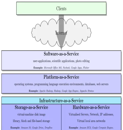
NIST categorises cloud services into three different categories in different layers of service. The service layout which determines what is being provisioned is depicted in Fig. 2.2. User can access these services through the internet using a client device such as a web browser or a program interface. These services from bottom-up are:

Infrastructure-as-a-Service (IaaS) provides the physical infrastructure of cloud computing. This category itself is divided into two subcategories: Hardware-as-a-Service (HaaS) and Storage-as-a-Service. HaaS provides the processing, memory, networking and all other fundamental things that the user can deploy and run an arbitrary software on them. They are provided in the form of

Virtual Machine (VM) instances. User can create VMs of desired configuration and install arbitrary software tools and interfaces on them. The latter provides virtualised storage in the form of raw disk space or object storage. The network is provided in the form of virtualised network that connects VMs to the internet or a private network. User does not control the cloud infrastructure, but only

(41)

Clients

Internet

Software-as-a-Service

user-applications, scientific applications, photo editing

Example:Microsoft Office 365, Facbook, Google Apps, Flicker

Platform-as-a-Service

operating systems, programming language execution environments, databases, web servers

Example:Apache Hadoop, Hadoop, Google App Engine, Appache Stratos

Infrastructure-as-a-Service

Storage-as-a-Service

virtual-machine disk image library, block and file-based storage

Example:Amazon S3, Google Drive, DropBox

Hardware-as-a-Service

Virtualised Servers, Network, IP addresses, Virtual local area networks

Example:Amazon EC2, Google Compute Engine.

Figure 2.2: The general reference model of the cloud.

the operating system, VMs behaviour and software installed on them. She/He has a limited access over the networking capabilities such as firewall settings.

Platform-as-a-Service (PaaS) offers services such as computing platform, run-time environments, databases, and web servers. It provides a framework for the software and application developers to be able to develop and customise their applications and software. These services are backed by a core middleware platform that is responsible for creating the abstract environment where ap-plications are deployed and executed [BVS13]. It means that service provider manages runtime environment, middleware, operating system, networking, fault tolerance, storage, etc., but users only concentrate on their application development and logic of their work.

Software-as-a-Service (SaaS) layer is build on the top of PaaS. It provides access to software applications which are referred to as on-demand software. Common

(42)

example are Adobe Photoshop, and Microsoft Office. Customers run these application on the cloud instead of a local desktop computer. These applications are usually shared among different users. Customers do not need to worry about installation, maintenance and running of the applications and it is the responsibility of the service provider. Users use a web interface program to access these services.

Users pay for the cloud services. The pricing model for the above services are described asdollar per hour and the cost is different based on the type of the service requested.

NIST provides five essential characteristics of the cloud as follows:

1. On-demand self service: A consumer can access computing resources automati-cally without requiring any human interaction.

2. Broad Network Access: Services and capabilities are available over the network and can be accessed through standard mechanisms anywhere regardless of the type of the device customers use.

3. Resource Pooling: The provider’s computing resources are pooled to serve multiple consumers using a multi-tenant model. Different physical and virtual resources are dynamically assigned and reassigned according to the consumer’s demand. Consumers have no control over the exact location of the provided resources, but they might be able to specify location at a higher level of abstraction.

4. Rapid Elasticity: Resources can scale dynamically and rapidly both inward and outward based on the demand. From the customer’s point of view, the services are unlimited and can be requested at any time.

5. Measured Service: Cloud systems automatically control and optimize resource use by leveraging a metering capability at some level of abstraction appropriate to the type of service (for example storage, processing, bandwidth, and active user accounts). Resource usage can be monitored, controlled, and reported