Bayesian single- and multi- objective optimisation with nonparametric priors

(1)

Bayesian single- and

multi-objective optimisation with

nonparametric priors

Amar Shah

Department of Engineering

University of Cambridge

This dissertation is submitted for the degree of

Doctor of Philosophy

(2)

(3)

Acknowledgements

It has been a privilege to be able to undertake a doctoral degree at such a prestigious institution. Many individuals and organisations have influenced me to get to this position. Here I would like to acknowledge a few of them. My lifelong gratitude to

My Phd supervisor, Zoubin Ghahramani, for education & inspiration, My colleagues from CBL & worldwide, for conversation & collaboration, My college, St John’s, for accommodation & sustentation,

My many friends and family for animation & stimulation, and My parents for building my foundation & overseeing its fortification.

(4)

(5)

Abstract

Optimisation is integral to all sorts of processes in science, economics and arguably underpins the fruition of human intelligence through millions of years of optimisation, orevolution. Scarce resources make it crucial to

max-imise their efficient usage. In this thesis, we consider the task of maximising unknown functions which we are able to query point-wise. The function is deemed to be costly to evaluate e.g. larger run time or financial expense,

requiring a judicious querying strategy given previous observations.

We adopt a probabilistic framework for modelling the unknown function and Bayesian non-parametric modelling. In particular, we focus on the Gaussian

process (GP), a popular non-parametric Bayesian prior on functions. We

motivate these choices and give an overview of the Gaussian process in the introduction, and its application to Bayesian optimisation.

A GP’s behaviour is intimately controlled by the choice of kernel or

co-variance function, typically chosen to be a parametric function. In chapter 2 we instead place a non-parametric Bayesian prior, known as an Inverse Wishart process prior, over a GP kernel function, and show that this may be marginalised analytically leading to a Student-t process (TP). Furthermore

we explore a larger class of elliptical processes, and show that the TP is

the most general for which analytic calculation is possible, and apply it successfully for Bayesian optimisation.

The remainder of the thesis focusses on various Bayesian optimisation set-tings. In chapter 3, we consider a setting where we are able to evaluate a function at multiple locations in parallel. Our approach is to consider a measure of information,entropy, to decide which batch of points to evaluate

(6)

a function at next. We similarly apply information gain for multi-objective

Bayesian optimisation in chapter 4. Here, one wishes to find a Pareto fron-tier of efficient settings with respect to several different objectives through

sequential evaluation. Finally, in chapter 5 we exploit the idea that in a multi-objective setting, functions arecorrelated, incorporating this belief in

(7)

Chapter 1

Introduction

This thesis is about non-parameteric function modelling with Bayesian pri-ors for the purpose of Bayesian optimisation. In this chapter, we begin by providing a high level historical overview of machine learning including research interest in neural networks and kernel machines. Next we introduce Bayesian reasoning, Gaussian process and Bayesian optimisation, before listing the subsequent contributions of this thesis in the remaining chapters. The core of machine learning is the development of statistical and com-putational methods for pattern recognition of data. A practitioner may wish to use a trained model to make predictions or decisions when presented with new unseen data, which is only possible when the model has a good

inductive bias, or generalisability.

Humans collect data about the world through continual interaction with it and develop the ability to predict the results of new actions. Therefore, techniques in machine learning are often inspired by human learning, for example, the perceptron [Rosenblatt, 1962] was inspired by a model of a human neuron [McCulloch and Pitts, 1943]. Neural networks began to be popularised in the 1980s, a key attraction being their ability to adapt basis functions, as opposed to traditional linear models with fixed basis functions [Rumelhart et al., 1986]. The expressiveness and seeming flexibility of neural network based models came at the cost of interpretability; there lacked a principled framework for making key modelling choices, which could affect

(12)

performance drastically in ways which were often difficult to explain. In the 1990s, kernel methods grew in popularity [Cristianini and Shawe-Taylor, 2000]. Kernel methods provided a way to consider infinitely many fixed basis functions whilst utilising finite resources, thanks to the kernel

trick, which implicitly represents inner products of basis function

representa-tions of data points using a kernel matrix [Hofmann et al., 2008].

A successful kernel based, Bayesian modelling tool for modelling non-linear

functions is the Gaussian process [Rasmussen and Williams, 2006], which

we discuss in more detail in the next subsections. In the machine learning community, Gaussian process research really spawned from the interest in neural networks. In fact, Neal [1995] argued that since model performance improved with the ability to account for additional structure in data, that we should pursue the limits of large models. He went on to show that a Gaussian process is in fact the limit of a particular Bayesian neural network architecture, as the number of hidden units tends to infinity. Gaussian process kernel machines are typically not able to scale to the size of today’s large datasets. Simplifying assumptions have been studied to improve scal-ability [Williams and Seeger, 2001; Csató and Opper, 2002; Snelson and Ghahramani, 2006], but Gaussian processes appear to be most useful in a

low to medium data setting. Bayesian optimisation is the task of finding

the maximum of a black-box function through a small number of sequential evaluations, a task well suited to the Gaussian procees and a key focus of this thesis.

1.1

Parametric Modelling

In this section we briefly illustrate the differences between frequentist and Bayesian reasoning in a regression task, in order to subsequently motivate a Bayesian approach to function optimisation. Suppose we have a set of observation pairs {xi, yi}ni=1 where yi is the scalar observed output for a known input vector xi, and that we wish to predict the output y∗ at a new input x∗. The outputs may represent house prices for given inputs such as

(13)

1.1 Parametric Modelling 3 location, house size, number of bedrooms, etc.

A typical statistical approach to learn the mapping from inputs, x, to

outputs, y, is to consider a class of functions which are controlled by a set

of parameters, and learning the parameter values which lead to the best

fit of the training data, for example by minimising the difference between predictions and true observed values. A simple class of functions which is able to learn linear trends is a linear model of the form f(x,w) = w⊤x,

where w are the parameters, or weights. For more complicated tasks, we

may use a linear model with a vector of fixed non-linear basis functions, or features ϕ(x) = [ϕ1(x), ϕ2(x), ..., ϕk(x)], with f(x,w) =w⊤ϕ(x). This is

a linear model, since f is a linear function with respect to the parameters,

but not necessarily with respect to the input space.

A common quantity to want to minimise for regression tasks where outputs are in a continuous space is

E(w) = 1 n n X i=1 (f(xi,w)−yi)2, (1.1)

the mean squared error of the predictions of the model over the training

data set. It is usually possible to minimise E(x) using gradient descent.

Often the output observations are modelled as being noisy, for example, a

reading instrument used to measure the output of a particular process may inherently have a limit as to its accuracy due to hardware factors. For the purposes of our example, we will continue to assume noiseless observations. A fundamental issue with the framework we have outlined above, is that for

k (the number of features) very large, for examplek ≫n, minimising (1.1)

may lead to the model overfitting. This is where f(x,w) focuses on being

able to reproduce the training data very well, caring too much on the random nuances of the training data rather than the true underlying trend, which hurts generalisation to new data. Whilst largerk leads to a more expressive

regression model, it also makes overfitting more likely. A typical approach used to control the level of overfitting, is to add a complexity penalty term to the error being minimised. For example, the original objective can be

(14)

modified to ˜ E(w) = 1 n n X i=1 (f(xi,w)−yi)2+λw⊤w, (1.2) for a positive scalar λ. Introducing a penalty term as we have done here

is called regularisation, the extra term acts so as to discourage weights

from being too large, which in turn limits the amount of overfitting. The

question becomes, “how should one set λ?” so as to trade off the error

and regularisation terms. A standard way to answer this question, is to take a fraction of the training set and place it aside as avalidation set. We

would proceed to train on the remaining data with different values ofλ, and

validate the model by computing the error on the validation set. A search is performed over λ to minimise the error on the validation set. This process

is called cross validation. In practice, it is unclear how one should decide

on what the validation set should be, and how many different settings of λ

should be validated with.

A very different approach to inference and regularisation is a Bayesian

one, where probability distributions are used to represent subjective un-certainty of an inference algorithm [MacKay, 2003; Jaynes, 2003; Barber, 2012; Gelman et al., 2014]. Specifically, we place a prior distribution on

the weights, p(w), and now model each yi as a sample from probability distribution e.g. N(f(xi,w), σ2) for some parameter σ. Bayes’ rule tells us how to compute the posterior distribution of weights given the observed data pw|{xi, yi}ni=1 ∝p(w) n Y i=1 p(yi|w,xi). (1.3)

We subsequently may make a mean prediction at a new input point x∗

by computing an integral Ep(w|{xi,yi}n_i=1)[f(x∗,w)], an example of Bayesian

model averaging, since we are averaging the prediction over multiple function models based on how likely they are given the observed data. This averag-ing prevents overfittaverag-ing as we are no longer consideraverag-ing one explanation of the data, as was the case when optimising (1.1). More generally, we may compute an entire probability distribution for our prediction at a new test point,py∗|x∗,{xi, yi}ni=1

, which enables us to consider all sorts of statistics about the prediction including the variance, mode, median, etc. Having

(15)

1.2 An Introduction to Gaussian Processes 5 an entire predictive distribution over new outputs is crucial for Bayesian decision making. The stochastic nature of predictions under a Bayesian framework reflects the uncertainty in modelling, which at a low level may

come directly from measurement errors, or at a higher level from reasoning about which model structure is ideal for the task. The probabilistic approach uses probability theory to express all forms of uncertainty. Probability theory is the mathematical language for representing and quantifying uncertainty [Ghahramani, 2015].

In this section we have discussed parametric models, which have a fixed representation capacity even as the number of datapoints increases. Non-parametric models do not have a finite number of parameters, in fact, as the number of data points increases, so do the number of parameters. The Gaussian process is a non-parametric Bayesian model which we introduce in the next section.

1.2

An Introduction to Gaussian Processes

Gaussian processes form a class of non-parametric stochastic processes over the space of functions [Rasmussen and Williams, 2006]. Unlike parametric models, the representational complexity of a Gaussian process (GP) grows with the number of observations. This is one of the many reasons which make GPs a popular choice for function modelling.

We proceed to provide a brief introduction to Gaussian process applica-tions to statistical regression. Readers wishing to explore GPs in more detail should benefit from referring to Rasmussen and Williams [2006].

1.2.1

Definition

A Gaussian process is a collection of random variables, of which any finite number are jointly Gaussian distributed. Let f :X → R. We write

(16)

to denote thatf follows a Gaussian process withmean function m(x), and

covariance functionk(x,x′), which fully specify the Gaussian process. The

function value f(x) has mean m(x) and has covariance with some other

function valuef(x′) defined byk(x,x′). Therefore, forX ≡[x1, ...,xn]⊂ X,

if we write fi ≡f(xi) andf ≡[f1, ..., fn]⊤, we have that

f|X ∼ N(m,K), (1.5)

where m≡[m(x1), ..., m(xn)]⊤ and K is a matrix with (i, j) entryKi,j =

k(xi,xj).

1.2.2

Gaussian Processes for Regression

Regression problems are core to statistical inference and machine learning. The goal is to learn a mapping from inputs to outputs based on a set of observed input-output pairs{xi, yi}ni=1. A typical application of learning this

mapping is to subsequently be able to predict an outputy∗ at a new test input

x∗. We describe how one may use a Gaussian process and Bayesian inference to respectively model and learn the function mapping from inputs to outputs. As we described previously, Bayesian inference consists of placing a prior distribution on parameters of interest, observing data and finally computing the posterior belief about parameters given the data. In regression tasks, the goal is to infer the function which maps inputs to outputs. A para-metric approach to Bayesian regression is to consider a family of functions parametrised by a finite set of random variables over which inference is per-formed. A less confined approach to Bayesian inference would be to directly specify a prior over an infinite-dimensional space of functions, instead of implicitly specifying a prior over functions via parameters [Orbanz and Teh, 2011].

A Gaussian process is a very popular choice as a prior over continuous

functions. Suppose f ∼ GP(m, k) and that we evaluate the function at

points x1, ...,xn ∈ X, then f|x ∼ N(m,K) as described above. Further suppose that each input location xi, we observe a real value yi which is

(17)

1.2 An Introduction to Gaussian Processes 7

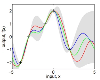
Fig. 1.1 Gaussian process posterior from 5 noiseless observations (plus signs). Coloured lines represent some possible functions to explain the observed data. The shaded region represents a 95 % predictive interval of where the function lies given observations. Figure from Rasmussen and Williams [2006].

stochastically dependent on the underlying function value f(xi). Bayes’

theorem informs us on how to obtain a posterior distribution of the function values at locationsxi given the observations yi:

p(f|y,X) = p(y|f)p(f|X)

p(y|X) =

p(y|f)N(f;m,K)

p(y|X) . (1.6)

A typical scenario is that the observations yi are simply the true function values corrupted by Gaussian noise, i.e. yi|fi ∼ N(fi, σ2). In this case, since both the likelihood p(yi|fi) and the prior p(f) are Gaussian, we can analytically compute the posterior distribution

f|y,X ∼ Nm+K(K+σ2I)−1(y−m),K−K(K+σ2I)−1K, (1.7)

which is in fact multivariate Gaussian distributed. Figure 1.1, taken from Rasmussen and Williams [2006], shows an example of some possible functions which could explain 5 noiseless observations, along with a 95 % predictive interval.

(18)

1.2.3

Gaussian Process Prediction

Whilst the posterior distribution of the functionf at observed input locations

X is useful, what is often of more interest is the predictive distribution

at new input locations. Let X∗ ≡ {x∗

1, ...,x

∗

n′} ⊂ X be a set of new

input locations. Let f_i∗ ≡ f(x∗_i) and f∗ ≡ [f₁∗, ..., f_n∗′]⊤. Further let the

concatenation of old and new input locations be X+ ≡ X ∪X∗, and let

f+ ≡ [f1, ..., fn, f1∗, ..., f

∗

n′]⊤. We write m∗ ≡ [m(x₁∗), ..., m(x∗_n′)]⊤ and m₊

as the concatenation of mandm∗. Further let K+ be a (n+n′)×(n+n′)

covariance matrix such that

K+=

_K _K′

K′⊤ K∗

, (1.8)

where K_i,j∗ = k(x_i∗,x∗_j) for i, j ∈ {1, ..., n′}, and K_i,j′ = k(xi,x∗j) for i ∈

{1, ..., n} and j ∈ {1, ..., n′}. Then p(f∗|y,X+) = Z p(f∗|f,X+)p(f|y,X)df, (1.9) and f∗|y,X+∼ N K′⊤(K+σ2I)−1(y−m) +m∗, (1.10) K∗−K′⊤(K+σ2I)−1K′ . (1.11)

Thus the posterior predictive distribution of a Gaussian process conditioned on observations is itself a Gaussian process.

1.2.4

Hyperparameter Learning

The behaviour of a draw from a Gaussian process prior is predominantly encoded in the choice of the covariance function, k. Typically, the Gaussian

process mean is chosen to be zero (or constant), and the covariance function is chosen to be parametric, such that k = kθ, for some set of parameters

θ. The parameters of the covariance function are often referred to as

hyperparameters of the Gaussian process model. Hyperparameters control the nature of the covariance between points in X, for example, length-scale

(19)

1.3 An Introduction to Bayesian Optimisation 9

|xd−x′d|. The hyperparameters can be learnt by maximising likelihood, i.e. by optimising p(y|X, θ) =−1 2y⊤(Kθ+σ2I)−1y− 1 2log|Kθ+σ2I| − n 2log 2π (1.12) with respect to θ by gradient ascent. Alternatively, one may apply a fully

Bayesian treatment to the hyperparameters by imposing a prior distribution on them, and sampling from the posterior

p(θ|y,X)∝p(y|X, θ)p(θ). (1.13)

1.3

An Introduction to Bayesian

Optimisa-tion

Many tasks in engineering and science can be abstractly described in terms of optimising a nonlinear function f(x) over a compact set X ⊂Rd_{. More} precisely, the task can be described as

max

x∈X f(x). (1.14)

In many instances,f is known in analytically and may also be differentiable,

in which case gradient based optimisation is often employed to find the

maximum of the function. However, there exist many scenarios where f

is not known analytically, and may only be evaluated pointwise through a simulation or process requiring many resources e.g. time or money.

In a scenario where pointwise evaluation is costly, a strategy of evaluating at points in X uniformly at random is naive and wasteful, and would converge

to large values of f far too slowly as the dimensionality of the input space

increases. Letx+ _{denote the best observed input location through sequential}

evaluation, and let x∗ denote the true maximiser of the functionf. In fact,

Betrò [1991] showed that an objective function with Lipschitz continuity

C would require O(C/2ϵ)d _{random uniform evaluations to ensure that}

(20)

Algorithm 1 Bayesian Optimisation 1: D ← ∅ 2: for t= 1,2, ..., T do 3: xt←argmaxx∈X u(x|D) 4: ft←f(xt) 5: D ← D ∪ {x_t, ft} 6: x+ _←argmax x∈ x1:Tf(x) 7: return x+

A Bayesian approach to optimising f, would be to model it by placing

a prior distribution over it, which would be updated sequentially using Bayes’ rule as function evaluations are observed. The posterior model off

given function evaluations is subsequently used to decide where in the input

domain, X, to evaluate the function next, in order to maximise a chosen

analytically tractable criterion which trades off exploration and exploita-tion. The criterion, u(x), is often referred to as the acquisition function.

A basic version of the Bayesian optimisation procedure is outlined in Al-gorithm 1 and illustrated in Figure 1.2 taken from [Brochu et al., 2009], which offers a nice and more thorough introduction to Bayesian optimisation. Bayesian optimisation research has been fuelled by many successful applica-tions in a diverse range of tasks. A few such successes are listed below:

• Robotics and reinforcement learning. Parametrising a robot’s

gait parameters allows you to optimise over its velocity or smoothness using Bayesian optimisation [Lizotte, 2008]. Similarly, robotic policy parametrisation and search techniques can be used to navigate a robot through landmarks whilst minimising uncertainty about location and map estimation [Martinez-Cantin et al., 2007].

• Natural language, processing and text. Bayesian optimisation

has been used to improve text extraction [Wang et al., 2014] and to tune representations for general text and language tasks [Yogatama and Smith, 2015].

• Sensor placement. Meteorological sensors can be expensive to ob-tain, so intelligent placement of them for the task at hand is useful.

(21)

1.3 An Introduction to Bayesian Optimisation 11 Bayesian optimisation has been used to tackle this problem [Garnett et al., 2010]. For mobile sensing, a cost can be associated in mak-ing a measurement (e.g. on a unmanned autonomous vehicle), this cost can be incorporated in decision making processes using Bayesian optimisation [Marchant and Ramos, 2012].

• Automatic machine learning. The goal is to automatically search over hyperparameters of machine learning algorithms for a given task. For example, when training a neural network, one has to choose a learning rate, momentum, weight decay, etc. Cross validation can be very expensive when a lot of parameters have to be searched over. Bayesian optimisation has recently been successfully applied to search over the space of hyperparameters, in some cases finding state of the art settings [Snoek et al., 2012].

The two key design choices required for implementing a Bayesian optimisation algorithm are: (i) the model forf, and (ii) theacquisition function to decide

where to evaluate the function next. We discuss each of these choices in the following subsections.

1.3.1

Model Choice for

f

Gaussian processes have been the most popular choice of prior over the

function f as they are non-parametric and permit analytically tractable

computation, as we will see in the next subsection. The use of Gaussian process priors for Bayesian optimisation began in the late 1970s [O’Hagan, 1978; Zilinskas, 1980].

The choice of covariance function is integral to the Gaussian process prior as it determines the smoothness properties of drawn samples. Various forms of covariance functions are discussed in Rasmussen and Williams [2006]. For isotropic function modelling, the squared exponential kernel with single

hyperparameter θ is most common, and defined as

k(x,x′) = exp

− 1

2θ2||x−x

(22)

acquisition max acquisition function (u(·)) observation (x) objective fn (f(·)) t = 2 new observation (xt) t = 3 posterior mean (µ(·)) posterior uncertainty (µ(·)±σ(·)) t = 4

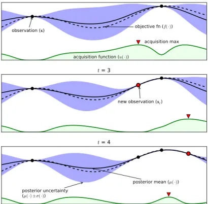
Figure 1: An example of using Bayesian optimization on a toy 1D design problem.

The figures show a Gaussian process (GP) approximation of the objective function over four iterations of sampled values of the objective function. The figure also shows the acquisition function in the lower shaded plots. The acquisition is high where the GP predicts a high objective (exploitation) and where the prediction uncertainty is high (exploration)—areas with both attributes are sampled first. Note that the area on the far left remains unsampled, as while it has high uncertainty, it is (correctly) predicted to offer little improvement over the highest observation.

The posterior captures our updated beliefs about the unknown objective func-tion. One may also interpret this step of Bayesian optimization as estimating

the objective function with a surrogate function (also called a response

sur-face), described formally in§2.1 with the posterior mean function of a Gaussian

process.

To sample efficiently, Bayesian optimization uses an acquisition function to

determine the next location xt+1 ∈ A to sample. The decision represents an

automatic trade-off between exploration (where the objective function is very

uncertain) and exploitation (trying values of x where the objective function is

expected to be high). This optimization technique has the nice property that it aims to minimize the number of objective function evaluations. Moreover, it is likely to do well even in settings where the objective function has multiple local maxima.

3

Fig. 1.2 An example of Gaussian process based Bayesian optimisation on a 1D objective to be maximised. Figures show 3 iterations of sampled values from the objective function from top to bottom. Observations are represented by dots, the true objective is the dotted line, the GP posterior mean and 95 % predictive interval are given by the dark solid lines and the purple shaded regions respectively. The green line at the bottom of each plot shows the acquisition function at each iteration. The acquisition is high where the GP predicts a high function value (exploitation) and where the predictive uncertainty is high (exploration). Figure from Brochu et al. [2009].

Most applications require anisotropic models which do not assume differences

in each component of x contribute to the covariance equally. In such a

scenario, the squared exponential with automatic relevance determination

(ARD) hyperparameters θ is a popular choice, defined as

k(x,x′) = exp − 1 2(x−x ′₎⊤_diag( θ)−2(x−x′) , (1.16)

where diag(θ) is a diagonal matrix with dth diagonal entry_θd. We can see

(23)

1.3 An Introduction to Bayesian Optimisation 13 less dependant on variations in the dth dimension of x, hence the kernel

function determines the relevance of each input dimension. One drawback of the squared exponential kernels is that they lead to very smooth functions which are infinitely differentiable. The Matérn kernel [Matérn, 1986] attempts to alleviate this problem by incorporating a smoothness parameter ζ, and is

defined as k(x,x′) = 1 2ζ−1Γ(_ζ) 2qζ||x−x′|| ζ Hζ 2qζ||x−x′|| (1.17) where Γ(.) and Hζ(.) are the Gamma function and the Bessel function of

order ζ. As ζ → ∞, the Matérn kernel reduces to the squared exponential

kernel. It is common to incorporate ARD hyperparameters into the Matérn kernel in practice. Kernels can be formed by composing other kernels.

1.3.2

Acquisition Functions

Theacquisition function controls the search for the optimum of the unknown

objective function given the model. Typically, an acquisition functionu(x|D)

defines the current expected utility of evaluating f at xgiven the observed

data so far, D, is defined such that values of high acquisition correspond to

input locations which offer more utility in evaluating the function at next.

Hence, maximising the acquisition function tells one where to evaluate f

next i.e. xt= argmaxxu(x|D).

In this subsection, we will describe 3 of the most common choices of acqui-sition functions for Bayesian optimisation tasks. We assume a Gaussian

process prior over the function f, and that we have observed the pairs

D = {xs, fs}Ts=1, with x+ = argmaxx∈x1:Tf(x). We denote the posterior

mean and covariance of f given observations D at location xas µ(x) and

σ(x)2_.

Kushner [1964] suggested maximising the probability of improving over the current best evaluation f(x+_{) with some margin,} _τ _≥ _{0, defining an}

(24)

acquisition function uPI(x|D) =P(f(x)≥f(x+) +τ) = Φ µ(x)−f(x+)−τ σ(x) ! (1.18) where Φ(.) is the standard normal cumulative distribution function. Large

values of τ lead to more exploration whilst small values encourage

exploita-tion, leading Kushner to recommend a schedule for τ such that it starts out

fairly high in the optimisation procedure and is decreased to zero as the algorithm progresses. Note that the probability of improvement acquisition function is indeed differentiable with respect to x, making gradient ascent

of the acquisition function possible.

Jones [2001b] studied the impact of the τ parameter on the performance of

Bayesian optimisation algorithm and concluded that it was highly sensitive. A more satisfying approach would weigh up the magnitude of improvement with the probability of improvement. In this vein, Mockus et al. [1978] defined the expected improvement over the current best evaluation as

uEI(x|D) = E

h

max

f(x)−f(x+),0i

=σ(x)hκ(x)Φ(κ(x)) +ϕ(κ(x))i (1.19)

where κ(x) =µ(x)−f(x+)/σ(x) and ϕ(.) is the standard normal density

function. The expected improvement acquisition function elegantly weighs up both the probability and magnitude of improvement over the current best. Another fairly simple way to trade off exploration and exploitation is to maximise an upper confidence bound of the form

uUCB(x|D) = µ(x) +βtσ(x) (1.20)

where βt isO

√

dlogt[Srinivas et al., 2010]. Note that each of the

acquisi-tion funcacquisi-tions presented here are myopic, in the sense that they maximise a

quantity based on a one-step ahead reward. The task in Bayesian optimisa-tion is to find an optimiser withinT steps, or more concretely, to minimise

(25)

1.4 Contributions 15

f(x∗)−f(x+) afterT steps. However, sampling multiple steps ahead quickly

becomes computationally infeasible due to the combinatorial explosion of possibilities over multiple steps. Nevertheless, Ginsbourger et al. [2008] did analytically compute expected improvement for the two-step ahead problem. Bayesian optimisation is intimately related to the problem of multi-armed bandits, where at each time step, a decision maker chooses an action from an action set, at∈ A, and receives a reward rt from the environment. The ac-tions are commonly described as arms in an analogy to the choice a gambler makes when deciding between several slot machines (one armed-bandits), which has a random payoff dependent on the particular arm. The gambler chooses so as to maximise their long term reward, by exploiting arms which pay well and exploring arms for which we require more information [Robbins, 1952; Gittins, 1979]. There have been many successful applications of multi-armed bandits including clinical trials [Thompson, 1933] and scheduling [Veatch and Wein, 1996].

1.4

Contributions

Here I outline the key contributions in this dissertation. Most of the work has been published in peer-reviewed conferences, but additional details and derivations are included in this document.

Previously in this chapter, we introduced the Gaussian process. However, the Gaussian distribution is only one of a large class ofelliptical distributions.

In chapter 2, we explore the possibility of more general elliptical processes, and prove that the Student-t process is the most general elliptical process

which permits analytically tractable predictions. We subsequently show that the Student-t process is useful for applications with heavy tailed noise and

also for Bayesian optimisation.

In chapter 3 we develop a novel acquisition function for Bayesian opti-misation where we are able to evaluate an objective function at multiple points in parallel. The acquisition function uses the notion of information

(26)

gain and statistical entropy in deciding at which points to evaluate next. Our method is the only one known to us which is able to choose a batch of points together, rather than one by one in a greedy fashion.

A similar but modified entropy based approach can be used in the multi-objective optimisation setting. In chapter 4, we discuss the notion of a Pareto frontier of optimal points when jointly trying to optimise multiple objectives, and show how one can choose to evaluate multiple objectives at a location which maximises the information gain about the true Pareto frontier. Finally in chapter 5, we model correlations between objective functions for the purpose of multi-objective optimisation. This proves to be fruitful in realistic scenarios as the multiple objective one may wish to optimise jointly are typically inherently correlated. In this work, we consider a volume based generalisation of the expected improvement acquisition function, and derive an analytically tractable approximation to the desired acquisition function.

(27)

Chapter 2

Student-

t

and Elliptical

Processes

In the introduction, I discuss the Gaussian process and the parameters which control its behaviour. A key design choice in prescribing a Gaussian process prior is in the covariance function. Whilst the kernel function is almost always chosen to be a parametric function, in this chapter we consider a non-parametric, stochastic alternative called the inverse Wishart process

(IWP), which attempts to learn the most appropriate form of covariance

function based on the training data. Marginalising the IWP prior on the Gaussian process covariance function leads to a Student-t process.

A connection to a more general class called elliptical distributions is made,

and we construct a Student-t process via an alternative generative process,

shedding light on some of the redundancies of the inverse Wishart process framework. The GP with IWP covariance function is designed to be able to flexibly model the covariance between function points and therefore is ideally suited to Bayesian optimisation, which is our primary application area. The core of this chapter was research I conducted in collaboration with Andrew Gordon Wilson and Zoubin Ghahramani, and has been published at AISTATS [Shah et al., 2014]. The majority of the work including the param-eterisation of the IWP, the experiments and the geometric interpretation

(28)

of the IWP were developed by myself, whilst Andrew and Zoubin offered guiding thoughts and suggestions for applications.

2.1

Introduction

Gaussian processes are rich distributions over functions, which provide a Bayesian non-parametric approach to regression. Owing to their inter-pretability, non-parametric flexibility, large support, consistency, simple exact learning and inference procedures, and impressive empirical perfor-mances [Rasmussen, 1996], Gaussian processes as kernel machines have steadily grown in popularity over the last decade.

At the heart of every Gaussian process (GP) is a parametrised covari-ance kernel, which determines the properties of likely functions under a GP. Typically simple parametric kernels, such as the Gaussian (squared exponential) kernel are used, and its parameters are determined through marginal likelihood maximisation, having analytically integrated away the Gaussian process. However, a fully Bayesian non-parametric treatment of regression would place a non-parametric prior over the Gaussian process covariance kernel, to represent uncertainty over the kernel function, and to reflect the natural intuition that the kernel does not have a simple parametric form.

Likewise, given the success of Gaussian processes kernel machines, it is also natural to consider more general families of elliptical processes [Fang et al., 1989], such as Student-t processes, where any collection of function

values has a desired elliptical distribution, with a covariance matrix con-structed using a kernel.

As we will show, the Student-t process can be derived by placing an inverse

Wishart process prior on the kernel of a Gaussian process. Given their intuitive value, it is not surprising that various forms of Student-t processes

have been used in different applications [Yu et al., 2007; Zhang and Yeung, 2010; Xu et al., 2011; Archambeau and Bach, 2010]. However, the

(29)

connec-2.1 Introduction 19 tions between these models and their theoretical properties, remain largely unknown. Similarly, the practical utility of such models remains uncertain. For example, Rasmussen and Williams [2006] wonder whether “the Student-t

process is perhaps not as exciting as one might have hoped”.

In this work, we precisely define and motivate the inverse Wishart pro-cess [Dawid, 1981] as a prior over covariance matrices of arbitrary size,

and derive a Student-t process (TP), from hierarchical Gaussian process

models. Our Student-t process has analytic forms of marginal and predictive

distributions, and analytic derivatives of the marginal likelihood. We go on to define elliptical distributions and corresponding processes, and prove that the Student-t process is the most general elliptically symmetric process with

analytic marginal and predictive distributions. This result allowed us to derive a new way of sampling from the inverse Wishart process, which intu-itively resolves the seemingly bizarre marginal equivalence between inverse Wishart and inverse Gamma priors for covariance kernels in hierarchical GP models. Unlike for a GP, we show that the predictive covariance of a TP depend on the values of training observations. Contrary to the Student-t

process described in Rasmussen and Williams [2006], we are able to derive an analytic TP noise model which can be used to separate signal and noise analytically.

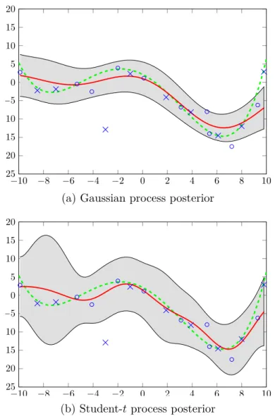
The TP appears to be more robust to change-points and model misspecifica-tion than the GP, and seems to have notably improved predictive covariance.

The TP further supports useful tail-dependence between distant function

values (which is separate from the choice of kernel). Both of these proper-ties make the TP particularly promising for Bayesian optimisation, where predictive covariance are especially important, as we show in Section 2.6.2. We proceed by introducing and defining the inverse Wishart process, and then apply it as a prior over a GP covariance function, leading to the Student-t process. Next we discuss elliptical distributions and processes,

drawing on some interesting connections to our initial approach to deriving a Student-t process. Finally we discuss some of our experimental findings

(30)

2.2

Inverse Wishart Process

We claim that the inverse Wishart distribution is an attractive choice of prior for covariance matrices of arbitrary size. The Wishart distribution is a probability distribution over Π(n), the set of real valued, n×n, symmetric,

positive definite matrices. Its density function is defined as follows.

Definition 1. A random Σ∈Π(n) is Wishart distributed with parameters

ν > n−1, K∈Π(n), and we write Σ∼Wn(ν,K) if its density is given by

p(Σ) =cn(ν,K)|Σ|(ν−n−1)/2_exp₋ 1 2Tr K−1Σ , (2.1) where cn(ν,K) = |K|ν/22νn/2Γn(_ν/2) −1 .

The Wishart distribution defined with this parametrisation is consistent under marginalisation. If Σ∼ Wn(ν, K), then any n1 ×n1 principal

sub-matrix, Σ11, is Wn1(ν, K11) distributed. This property is one which makes

the Wishart distribution appear to be an attractive prior over covariance matrices. Unfortunately the Wishart distribution suffers a flaw which makes it impractical for non-parametric Bayesian modelling.

Suppose we wish to model a covariance matrix using ν−1_Σ, with expected

value E[ν−1_Σ] =_K, and var[_ν−1_Σ

ij] =ν−1(K2ij+KiiKjj). Since we require

ν > n− 1, we must let ν → ∞ to define a process which has positive

semi-definite Wishart distributed marginals of arbitrary size. However, as

ν → ∞, ν−1_Σ tends to the constant matrix _K almost surely. Thus the

requirementν > n−1 prohibits defining a useful process which has Wishart

marginals of arbitrary size. Nevertheless, the inverse Wishart distribution

does not suffer this problem. Dawid [1981] parametrised the inverse Wishart distribution as follows:

Definition 2. A random Σ ∈ Π(n) is inverse Wishart distributed with

parameters ν ∈R+, K∈Π(n) and we write Σ∼IWn(ν,K) if its density is

given by p(Σ) = cn(ν,K)|Σ|−(ν+2n)/2_exp₋1 2Tr KΣ−1 , (2.2)

(31)

2.3 Deriving the Student-t Process 21

with cn(ν, K) = |K|

(ν+n−1)/2

2(ν+n−1)n/2Γn((_ν+_n₋1)_/2).

If Σ ∼ IWn(ν,K), Σ has mean and covariance only when ν > 2 and

E[Σ] = (ν−2)−1_K. Both the Wishart and the inverse Wishart distributions

place prior mass on every Σ ∈ Π(n). Furthermore Σ ∼ Wn(ν,K) if and

only if Σ−1 _∼IWn(_ν₋_n+ 1_,_K−1).

Dawid [1981] shows that the inverse Wishart distribution defined as above is consistent under marginalisation. IfΣ∼IWn(ν,K), then any principal submatrix Σ11 will be IWn1(ν,K11) distributed. Note the key difference in

the parametrisation of both distributions: the parameter ν does not need

to depend on the size of the matrix in the inverse Wishart distribution. These properties are desirable and motivate defining a process which has inverse Wishart marginals of arbitrary size. Let X be some input space and

k :X × X →R a positive definite kernel function.

Definition 3. Σis an inverse Wishart process onX with parametersν ∈R+

and base kernel k : X × X →R if for any finite collection x1, ..., xn ∈ X,

Σ(x1, ..., xn)∼IWn(ν,K) where K∈ Π(n) with Kij =k(xi, xj). We write

Σ∼IWP(ν, k).

In the next section we use the inverse Wishart process as a non-parametric prior over kernels in a hierarchical Gaussian process model.

2.3

Deriving the Student-t

Process

Gaussian processes (GPs) are characterised by a mean function and a kernel function. Practitioners tend to use parametric kernel functions and learn their hyperparameters using maximum likelihood or sampling based methods. We propose placing an inverse Wishart process prior on the kernel function, leading to a Student-t process.

For a base kernel function kθ parametrised by θ, and a continuous mean

(32)

σ ∼IWP(ν, kθ)

y|σ ∼GP(ϕ,(ν−2)σ), (2.3)

where σ is an infinite dimensional covariance function defined on X × X.

Since the inverse Wishart distribution is a conjugate prior for the covariance matrix of a Gaussian likelihood, we can analytically marginalise σ in the

generative model of (2.3). For any collection of data y= (y1, ..., yn)⊤ with

We leverage this result to define a Student-t process as follows.

Definition 4. y∈Rn _{is multivariate Student-t} _{distributed with parameters}

ν ∈R+\[0,2], ϕ∈Rn and K∈Π(n) if it has density

p(y) = Γ( ν+n 2 ) ((ν−2)π)n2Γ(ν 2) |K|−1/2× 1 + (y−ϕ)⊤K−1(y−ϕ) ν−2 −ν+n₂ (2.5) We write y∼MVTn(ν,ϕ,K).

The mean and covariance of the MVT are easily computed using the genera-tive derivation:

E[y] =E[E[y|Σ]] =ϕ

cov[y] =E[E[(y−ϕ)(y−ϕ)⊤|Σ]] = E[(ν−2)Σ] =K. (2.6)

It is also straightforward to show that the Student-t is consistent under

marginalisation, which we do in the following Lemma.

(33)

2.3 Deriving the Student-t Process 23

Proof. Assume the generative process of equation 3 of the main text. Σ11

is IWn1(ν,K11) distributed for any principal submatrix ofΣ. Furthermore y1|Σ11 ∼ Nn1(0,(ν−2)Σ11) since the Gaussian distribution is consistent

under marginalisation. Hence y1 ∼MVTn1(ν, µ1,K11).

We are now able to define a Student-t process.

Definition 6. f is a Student-t process on X with parameters ν >2, mean

function Φ : X → R, and kernel function k : X × X → R if any finite

collection of function values have a joint multivariate Student-t distribution,

i.e. [f(x1), ..., f(xn)]⊤ ∼ MVTn(ν,ϕ,K) where K ∈ Π(n) with Kij =

k(xi, xj) and ϕ ∈Rn with ϕi = Φ(xi). We write f ∼TP(ν,Φ, k).

The Student-t process generalises the Gaussian process. In fact, a GP can

be seen as a limiting case of a TP as shown in the following Lemma. Lemma 7. Suppose f ∼TP(ν,Φ, k) and g ∼GP(Φ, k). Then f tends to g

in distribution as ν → ∞.

Proof. It is sufficient to show convergence in density for any finite collection

of inputs. Let y∼MVTn(ν,ϕ, K) and set β = (y−ϕ)⊤K−1(_y₋_ϕ) then

as ν→ ∞, p(y)∝ 1 + β ν−2 −(ν+n)/2 →e−β/2.

Hence the distribution ofy tends to a Nn(ϕ, K) distribution asν → ∞.

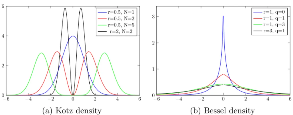
The ν parameter controls how heavy tailed the Student-t process is. Smaller

values ofν correspond to heavier tails. Asν gets larger, the tails converge to

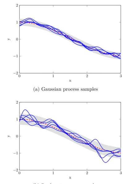
Gaussian tails. This is illustrated in prior sample draws shown in Figure 2.1. Notice that the samples from the TP tend to have more extreme behaviour than the GP, despite sharing the same mean and covariance functions.

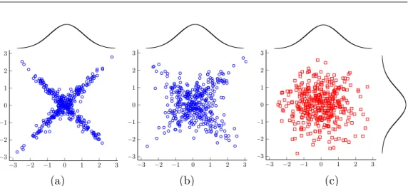
ν also controls the dependence between variables which are jointly Student-t

distributed, and not just their marginal distributions. In Figure 2.2 we show plots of samples which all have Gaussian marginals but different joint distributions determined by either a Student-t or a Gaussian copula. Note

(34)

0 1 2 3 −2 −1 0 1 2 x y 0 1 2 3 −2 −1 0 1 2 x y 1

(a) Gaussian process samples

0 1 2 3 −2 −1 0 1 2 x y 0 1 2 3 −2 −1 0 1 2 x y 1

(b) Student-t process samples

Fig. 2.1 Five samples (blue solid) from (a) GP(Φ, k) and (b) TP(ν,Φ, k),

with ν = 3. The mean and covariance functions are Φ(x) = cos(x) (red

dashed) and k(xi, xj) = 0.01 exp(−20(xi −xj)2) respectively. The grey shaded area represents a 95% predictive interval under each model.

Student-t copula is not an elliptical distribution, hence the non-elliptical

nature of Figure 2.2(a). Notice how the tail dependency of these distri-butions is controlled by ν. The dependency between y(xp) and y(xq) are

different depending on whether y is a TP or a GP, even if they share the

(35)

2.3 Deriving the Student-t Process 25 Manuscript under review by AISTATS 2014

−6 −5 −4 −3 −2 −1 0 1 2 3 4 5 6 0 0.5 1 1.5 2 2.5 3 1 −6 −5 −4 −3 −2 −1 0 1 2 3 4 5 6 0 0.5 1 1.5 2 2.5 3 1 −6 −5 −4 −3 −2 −1 0 1 2 3 4 5 6 0 0.5 1 1.5 2 2.5 3 1 −3 −2 −1 0 1 2 3 −3 −2 −1 0 1 2 3 −3 −2 −1 0 1 2 3 −3 −2 −1 0 1 2 3 −3 −2 −1 0 1 2 3 −3 −2 −1 0 1 2 3 1 −3 −2 −1 0 1 2 3 −3 −2 −1 0 1 2 3 −3 −2 −1 0 1 2 3 −3 −2 −1 0 1 2 3 −3 −2 −1 0 1 2 3 −3 −2 −1 0 1 2 3 1 −3 −2 −1 0 1 2 3 −3 −2 −1 0 1 2 3 −3 −2 −1 0 1 2 3 −3 −2 −1 0 1 2 3 −3 −2 −1 0 1 2 3 −3 −2 −1 0 1 2 3 1 − 6 − 5 − 4 − 3 − 2 − 1 0 1 2 3 4 5 6 0 0 . 5 1 1 . 5 2 2 . 5 3 1

Figure 2: Bivariate samples from a student-t copula withν= 3 (left), a student-t copula withν= 10 (centre) and a Gaussian copula (right). All marginal distributions are N(0,1) distributed.

Proof. It is sufficient to show convergence in den-sity for any finite collection of inputs. Let y ∼

MVTn(ν,φ, K) and setβ= (y−φ)>K−1(y−φ) then

p(y)∝1 + β

ν−2

−(ν+n)/2

→e−β/2

anν → ∞. Hence the distribution of ytends to a Nn(φ, K) distribution asν→ ∞.

Theνparameter controls howheavy tailedthe process is. The smaller it is, the heavier the tails. Asνgets larger, the tails converge to mimic Gaussian tails. This is illustrated in prior sample draws shown in Figure 1. Notice that the samples from the TP leave the 95% confidence band more often than the samples from the GP, a clear indicator of the heavier tails.

It is important to note thatνalso controls the nature of the dependence between variables which are jointly student-t distributed and not just the marginal distri-bution of points. In Figure 2 we show plots of samples which all have Gaussian marginals but different joint distributions. Notice how the tail dependency of the bivariate distributions is controlled byν.

4.2 Conditional distribution

We now derive the conditional distribution for a multivariate student-t distribution. Suppose y ∼

MVTn(ν,φ, K) and lety1andy2represent the first

n1 and remaining n2 entries of y respectively. Let β1 = (y1 −φ1)>K11−1(y1 −φ1) and β2 = (y2 − ˜ φ2)>K˜22− 1 (y2−φ˜2), where ˜φ2=K21K11−1(y1−φ1)− φ2and ˜K22=K22−K21K11−1K12.

Note thatβ1+β2= (y−φ)>K−1(y−φ). We have p(y2|y1) = p(y1,y2) p(y1) ∝1 +β1+β2 ν−2 −(ν+n)/2 1 + β1 ν−2 (ν+n1)/2 ∝1 + β2 β1+ν−2 −(ν+n)/2 (6)

Comparing this density to the one in equation 5, we note that y2|y1∼MVTn2 ν+n1,φ˜2,ν+β1−2 ν+n1−2× ˜ K22 . (7)

Asνtends to infinity, this predictive distribution tends to a Gaussian process predictive distribution as we would expect given Lemma 2. The predictive mean has the same form as for a Gaussian process predic-tive. The key difference is in the predictive covariance, which is a scaled version of the Gaussian process pre-dictive covariance.

A somewhat disappointing feature of the Gaussian process is that for a given kernel, the predictive co-variance of new samples does not explicitly depend on previous observations.

The scaling constant of the multivariate student-t pre-dictive covariance has an intuitive explanation. Note thatβ1is distributed as the sum of squares ofn1

inde-pendent MVT1(ν,0,1) distributions and henceE[β1] = n1. If the observed value ofβ1is larger thann1, the

predictive covariance is scaled up and vice versa. The magnitude of scaling is controlled byν.

The fact that the predictive covariance of the multi-variate student-t depends on the data is one of the key benefits of this distribution over a Gaussian one.

(a)

Manuscript under review by AISTATS 2014

−6 −5 −4 −3 −2 −1 0 1 2 3 4 5 6 0 0.5 1 1.5 2 2.5 3 1 −6 −5 −4 −3 −2 −1 0 1 2 3 4 5 6 0 0.5 1 1.5 2 2.5 3 1 −6 −5 −4 −3 −2 −1 0 1 2 3 4 5 6 0 0.5 1 1.5 2 2.5 3 1 −3 −2 −1 0 1 2 3 −3 −2 −1 0 1 2 3 −3 −2 −1 0 1 2 3 −3 −2 −1 0 1 2 3 −3 −2 −1 0 1 2 3 −3 −2 −1 0 1 2 3 1 −3 −2 −1 0 1 2 3 −3 −2 −1 0 1 2 3 −3 −2 −1 0 1 2 3 −3 −2 −1 0 1 2 3 −3 −2 −1 0 1 2 3 −3 −2 −1 0 1 2 3 1 −3 −2 −1 0 1 2 3 −3 −2 −1 0 1 2 3 −3 −2 −1 0 1 2 3 −3 −2 −1 0 1 2 3 −3 −2 −1 0 1 2 3 −3 −2 −1 0 1 2 3 1 − 6 − 5 − 4 − 3 − 2 − 1 0 1 2 3 4 5 6 0 0 . 5 1 1 . 5 2 2 . 5 3 1

Proof.It is sufficient to show convergence in den-sity for any finite collection of inputs. Let y ∼

MVTn(ν,φ, K) and setβ= (y−φ)>K−1(y−φ) then

p(y)∝1 + β

ν−2

−(ν+n)/2

→e−β/2

anν → ∞. Hence the distribution ofy tends to a Nn(φ, K) distribution asν→ ∞.

We now derive the conditional distribution for a multivariate student-t distribution. Suppose y ∼

MVTn(ν,φ, K) and lety1 andy2 represent the first

n1 and remaining n2 entries of y respectively. Let β1 = (y1−φ1)>K11−1(y1 −φ1) and β2 = (y2− ˜ φ2)>K˜22− 1 (y2−φ˜2), where ˜φ2=K21K11−1(y1−φ1)− φ2and ˜K22=K22−K21K−111K12.

Note thatβ1+β2= (y−φ)>K−1(y−φ). We have p(y2|y1) = p(y1,y2) p(y1) ∝1 +β1+β2 ν−2 −(ν+n)/2 1 + β1 ν−2 (ν+n1)/2 ∝1 + β2 β1+ν−2 −(ν+n)/2 (6)

Comparing this density to the one in equation 5, we note that y2|y1∼MVTn2 ν+n1,φ˜2,ν+β1−2 ν+n1−2× ˜ K22 . (7)

Asνtends to infinity, this predictive distribution tends to a Gaussian process predictive distribution as we would expect given Lemma 2. The predictive mean has the same form as for a Gaussian process predic-tive. The key difference is in the predictive covariance, which is a scaled version of the Gaussian process pre-dictive covariance.

inde-pendent MVT1(ν,0,1) distributions and henceE[β1] = n1. If the observed value ofβ1is larger thann1, the

(b)

Manuscript under review by AISTATS 2014

−6 −5 −4 −3 −2 −1 0 1 2 3 4 5 6 0 0.5 1 1.5 2 2.5 3 1 −6 −5 −4 −3 −2 −1 0 1 2 3 4 5 6 0 0.5 1 1.5 2 2.5 3 1 −6 −5 −4 −3 −2 −1 0 1 2 3 4 5 6 0 0.5 1 1.5 2 2.5 3 1 −3 −2 −1 0 1 2 3 −3 −2 −1 0 1 2 3 −3 −2 −1 0 1 2 3 −3 −2 −1 0 1 2 3 −3 −2 −1 0 1 2 3 −3 −2 −1 0 1 2 3 1 −3 −2 −1 0 1 2 3 −3 −2 −1 0 1 2 3 −3 −2 −1 0 1 2 3 −3 −2 −1 0 1 2 3 −3 −2 −1 0 1 2 3 −3 −2 −1 0 1 2 3 1 −3 −2 −1 0 1 2 3 −3 −2 −1 0 1 2 3 −3 −2 −1 0 1 2 3 −3 −2 −1 0 1 2 3 −3 −2 −1 0 1 2 3 −3 −2 −1 0 1 2 3 1 − 6 − 5 − 4 − 3 − 2 − 1 0 1 2 3 4 5 6 0 0 . 5 1 1 . 5 2 2 . 5 3 1

Proof.It is sufficient to show convergence in den-sity for any finite collection of inputs. Let y ∼ MVTn(ν,φ, K) and setβ= (y−φ)>K−1(y−φ) then

p(y)∝1 + β

ν−2

−(ν+n)/2

→e−β/2

anν → ∞. Hence the distribution ofy tends to a Nn(φ, K) distribution asν→ ∞.

We now derive the conditional distribution for a multivariate student-t distribution. Suppose y ∼ MVTn(ν,φ, K) and lety1andy2 represent the first

n1 and remaining n2 entries of y respectively. Let

β1 = (y1 −φ1)>K11−1(y1−φ1) and β2 = (y2− ˜ φ2)>K˜22− 1 (y2−φ˜2), where ˜φ2=K21K11−1(y1−φ1)− φ2and ˜K22=K22−K21K11−1K12.

Note thatβ1+β2= (y−φ)>K−1(y−φ). We have

p(y2|y1) =p(y1,y2) p(y1) ∝1 +β1+β2 ν−2 −(ν+n)/2 1 + β1 ν−2 (ν+n1)/2 ∝1 + β2 β1+ν−2 −(ν+n)/2 (6) Comparing this density to the one in equation 5, we note that y2|y1∼MVTn2 ν+n1,φ˜2,ν+β1−2 ν+n1−2× ˜ K22 . (7) Asνtends to infinity, this predictive distribution tends to a Gaussian process predictive distribution as we would expect given Lemma 2. The predictive mean has the same form as for a Gaussian process predic-tive. The key difference is in the predictive covariance, which is a scaled version of the Gaussian process pre-dictive covariance.

inde-pendent MVT1(ν,0,1) distributions and henceE[β1] =

n1. If the observed value ofβ1is larger thann1, the

(c)

Fig. 2.2 Uncorrelated bivariate samples from (a) a Student-t copula with ν = 3, (b) a Student-t copula withν = 10 and (c) a Gaussian copula (right).

All marginal distributions are N(0,1) distributed.

The conditional distribution for a multivariate Student-t has an analytic

form which we state and prove in Lemma 8.

Lemma 8. Suppose y ∼ MVTn(ν,ϕ,K) and let y1 and y2 represent the

first n1 and remaining n2 entries of y respectively. Then

y2|y1 ∼MVTn2 ν+n1,ϕ2˜ , ν+β1−2 ν+n1−2 ×K˜₂₂ , (2.7) where ˜ ϕ2 =K21K−111(y1−ϕ1) +ϕ2 β1 = (y1−ϕ1)⊤K11−1(y1−ϕ1), ˜ K22 =K22−K21K−111K12. Note that E[y2|y1] = ˜ϕ2, cov[y2|y1] = ν+β1 −2 ν+n1−2 ×K˜22.

(36)

Proof. Letβ2 = (y2−ϕ2˜ )⊤K˜22−1(y2−ϕ2˜ ).

Note thatβ1+β2 = (y−ϕ)⊤K−1(y−ϕ). We have

p(y2|y1) = p(y1,y2) p(y1) ∝ 1 + β1+β2 ν−2 −(ν+n)/2 1 + β1 ν−2 (ν+n1)/2 ∝ 1 + β2 β1+ν−2 −(ν+n)/2

Comparing this expression to the definition of a MVT density function gives the required result.

Asνtends to infinity, this predictive distribution tends to a Gaussian process

predictive distribution as we would expect given Lemma 7. Perhaps less intuitively, this predictive distribution also tends to a Gaussian process predictive asn1 tends to infinity. For n1 above 50, there typically would not

be a noticeable difference between the Student-t and Gaussian predictive

distribution. Therefore the Student-t process is interesting predominantly

in the low data setting.

The predictive mean has the same form as for a Gaussian process, con-ditioned on having the same kernel k, with the same hyperparameters. The

key difference is in the predictive covariance, which now explicitly depends on the training observations. Indeed, a somewhat disappointing feature of the Gaussian process is that for a given kernel with fixed hyperparameters, the predictive covariance of new samples does not depend on training ob-servations. Importantly, since the marginal likelihood of the TP in (2.5) differs from the marginal likelihood of the GP, both the predictive mean and predictive covariance of a TP will differ from that of a GP, after learning kernel hyperparameters.

The scaling constant of the multivariate Student-t predictive covariance