Computational Optimization Methods in Statistics, Econometrics and Finance
COMISEF WORKING PAPERS SERIES
WPS-042 24/08/2010
A comparative study of the
Lasso-type and heuristic
model selection methods
I. Savin
-A comparative study of the Lasso-type and
heuristic model selection methods
∗
Ivan Savin
Department of Economics, Justus Liebig University Giessen
Abstract
This study presents a first comparative analysis of Lasso-type (Lasso, adaptive Lasso, elastic net) and heuristic subset selection methods. Although the Lasso has shown success in many situations, it has some limitations. In particular, inconsistent results are obtained for pairwise strongly correlated predictors. An alternative to the Lasso is consti-tuted by model selection based on information criteria (IC), which remains consistent in the situation mentioned. However, these crite-ria are hard to optimize due to a discrete search space. To overcome this problem, an optimization heuristic (Genetic Algorithm) is ap-plied. Monte-Carlo simulation results are reported to illustrate the performance of the methods.
Keywords: Model selection, Lasso, adaptive Lasso, elastic net, heuristic methods, genetic algorithms.
∗Financial support from the German Academic Exchange Service (DAAD) and the EU Commission through MRTN-CT-2006-034270 COMISEF is gratefully acknowledged.
1
Introduction
The model selection process is crucial for the further analysis of any multiple regression model. Picking up too many regressors increases the variance of the constructed model, and taking fewer regressors than needed results in inconsistent estimates. In the last years the least absolute shrinkage and se-lection operator (Lasso) (Tibshirani 1996) has become a very popular method for simultaneous model selection and parameter estimation.
Among the Lasso’s main advantages are the combination of prediction accuracy and the parsimony of models built. The Lasso-type estimator out-performs simple application of parameter estimation methods (as, e.g., or-dinary least squares or method of moments) since it shrinks the coefficients of insignificant regressors towards zero. Hence, the resulting models concen-trate on the strongest effects and the total accuracy of the model forecast is increased. In addition, the Lasso solutions are more stable than other subset selection techniques based on the information criteria (IC) and step-wise strategies as, e.g., the general-to-specific approach (PcGets) discussed by Hendry and Krolzig (2005) and its bottom-up alternative (RETINA) an-alyzed by Perez-Amaral et al. (2003).
Another important advantage of the Lasso is its computational feasibil-ity. Since its computational cost hardly exceeds the complexity of one linear regression (Efron et al.2004), it is more attractive in comparison to classical model selection strategies that involve more intensive combinatorial search. However, the Lasso-estimator has some limitations. In particular, inconsis-tent results are obtained for highly correlated regressors (see Section 2).
In the last five years many studies have been devoted to methods revising and improving the initial Lasso concept. Since it is infeasible to describe them all in detail in this short introduction, I name only the most important ones from my perspective: the elastic net (EN) (Zou and Hastie 2005) and the adaptive Lasso (aLasso) (Zou 2006). A special case of the Lasso-type technique with the penalty term’s exponent less than one is analyzed by Knight and Fu (2000).
based on IC. In opposition to the Lasso, IC remain consistent even for data sets with correlated regressors. The IC’s main constraint is the computa-tional burden associated with the search for the optimum solution even for a moderate number of regressors. However, as is shown, e.g., by Maringer and Winker (2009), thanks to recent advances in heuristic optimization methods mimicking natural evolution processes, there are efficient algorithms able to select a model with at least a good approximation to the IC’s global opti-mum. To the best of my knowledge, this article is the first that compares the Lasso-type and the heuristic model selection methods. An important contri-bution of this study is the demonstration that in certain situations (e.g., if the portion of relevant predictors in a given data set is large) subset selection methods via heuristic algorithms can outperform the Lasso-type solutions.
The remainder of the paper proceeds as follows. Section 2 introduces both the Lasso-type methods and the heuristic model selection technique. Section 3 provides the results of our Monte-Carlo analysis and Section 4 illustrates an application to a cross-country growth model. Finally, Section 5 concludes.
2
Model selection strategies
2.1
Least absolute shrinkage and selection operator
The least absolute shrinkage and selection operator (Lasso) was introduced by Tibshirani (1996). Initially suggested as a constrained version of the ordi-nary least squares estimator, Lasso can be applied to a variety of estimation methods including, e.g., VAR-models (Hsuet al.2007) and GMM-estimators (Caner 2009). Numerous applications of this technique can be found in medicine, economics and other scientific fields (Foster et al. 2008, Hastieet al. 2009).
Let us consider the basic approach to the model selection problem for the following regression function:
where 𝛼 is an 𝑛-vector with all elements equal, 𝑋 is an 𝑛×𝑘 matrix of 𝑘
regressors and their values for 𝑛 observations, 𝛽 is a 𝑘×1 vector of their coefficients and 𝜀 is an 𝑛×1vector of residuals.
In (1) 𝑋𝑜𝑝𝑡 refers to the subset of all regressors one seeks to identify.
This might be the ‘true’ model in a Monte-Carlo simulation set-up or an optimal approximation to the unknown real data generating process. Let us assume that the predictors have been standardized to have mean zero and unit length, and that the response has mean zero:
𝑛 ∑ 𝑖=1 𝑦𝑖 = 0, 𝑛 ∑ 𝑖=1 𝑥𝑖𝑗 = 0, 𝑛 ∑ 𝑖=1 𝑥2𝑖𝑗 = 1, 𝑖= 1, ..., 𝑛, 𝑗 = 1, ..., 𝑘. (2) Hence, one can omit𝛼 without loss of generality. Then, the Lasso objec-tive function can be presented as follows:
ˆ 𝛽𝐿𝑎𝑠𝑠𝑜 = arg min 𝛽 [ ∥𝑦−𝑋𝛽ˆ∥22 +𝜆∥𝛽ˆ∥1 ] . (3)
While the first term in the right part of equation (3) is just the residual sum of squares (RSS), the second term with 𝜆 >0is the amount of shrinkage the Lasso applies to the sum of the absolute values of the coefficients.1 Hence,
the Lasso can be referred to as a special case of the Bridge regression approach (Frank and Friedman 1993) imposing an upper bound on the 𝐿𝑞-norm of the parameters (0< 𝑞 <∞) with 𝑞= 1: ∥𝛽ˆ∥𝑞= [ 𝑘 ∑ 𝑗=1 ∣𝛽𝑗∣𝑞 ]1/𝑞 . (4)
Equivalently to (3), the Lasso chooses𝛽ˆby minimizing RSS subject to a bound 𝑡 on the𝐿1-norm of the parameters:
ˆ
𝛽𝐿𝑎𝑠𝑠𝑜 = arg min 𝛽
∥𝑦−𝑋𝛽ˆ∥22 subject to ∥𝛽ˆ∥1≤𝑡 (5) 1𝜆 is a tuning parameter that can be defined using a data-driven method as, e.g., cross-validation.
with 𝑡 being inversely proportional to𝜆.
In the following the intuition behind the Lasso algorithm (a modification of the LARS algorithm) is briefly described.2 One starts with an empty model (all coefficients are set to zero) and identifies the predictor 𝑥𝜁 out of
the full set of 𝑘 regressors (ℐ) most correlated with the response 𝑦:
ˆ 𝜁 = arg max 𝜁 ∣ˆ𝑐𝜁∣, where ˆ𝑐𝜁 =𝑋 ′ ℐ(𝑦−ˆ𝜇0) (6)
with 𝜇ˆ=𝑋𝒜𝛽ˆbeing a prediction vector of regressors included in the model (respectively, one starts with 𝜇ˆ0 = 0).
Transferring the𝜁-regressor to the ’solution path’ (𝒜) one needs to ensure that the next predictor 𝑥𝜍 to be included in 𝒜 (𝑥𝜍 is the most correlated
covariate with the current residual) has as much correlation with 𝑦2−𝜇ˆ1 as
𝑥𝜁. In other words, 𝑦2 −𝜇ˆ1 has to ’bisect’ the angle between 𝑥𝜁 and 𝑥𝜍, so that 𝑐𝜁(𝜇ˆ1) =𝑐𝜍(𝜇ˆ1). To this end, one increases ˆ𝜇0 in the direction of 𝑥𝜁:
ˆ
𝜇1 =ˆ𝜇0+ˆ𝛾𝜁𝑥𝜁. (7) In theLARS algorithm ˆ𝛾𝜁 is taken as the smallest positive value, so that
another regressor can be included in the solution path fulfilling the condi-tion of ’equally correlated regressors’. Starting from the third predictor one employs an ’equiangular vector’ (𝑢𝒜) in (7) instead of the previous included
regressor (𝑥𝜁). The ’equiangular vector’ is a unit vector constructed based
on all covariates already transferred to 𝒜 (𝑋𝒜) generating equal angles with
the regressors.
In addition, the algorithm enforces that in each step𝜓 = 1,2, ...,Ψ(when a new regressor is included in 𝒜) the sign of all predictors’ estimates (𝑠𝒜)
in the Lasso solution 𝛽ˆmust agree with the sign of the current correlation3 ˆ
𝑐𝜓,𝒜 =𝑋′(𝑦−𝜇ˆ𝜓−1):
𝑠𝒜 =sign(ˆ𝑐𝒜) =sign(𝛽ˆ𝒜). (8)
2For a detailed (technical) explanation of all steps see Efronet al.(2004).
3Ψ is an additional stopping criteria limiting the maximum number of steps. In the LARS algorithmΨ = 8𝑘that is usually enough for all k to be included in𝒜.
If the restriction (8) is violated, the corresponding regressor𝑥𝜌is removed
from𝒜and, therefore, is removed from the calculation of the next equiangu-lar direction (𝑢𝒜). However, later𝑥𝜌 can be re-included in𝒜, but the order
of predictors in the solution path will be already different. This process con-tinues until all 𝑘 regressors are transferred to 𝒜, thus, ensuring that at each step 𝜓 only one regressor can be included or excluded from𝒜,𝑚𝑎𝑥(𝜓)≥𝑘. As a result, one obtains a piecewise-linear solution path in the tuning parameter𝜆 ∈[0,∞)with all𝛽ˆ’s set to zero at𝜆 =∞and equal to the OLS estimate at 𝜆= 0 (all 𝑘 covariates included).
Then, in order to select a single Lasso-solution out of 𝒜, tenfold cross-validation minimizing the prediction error (PE) of 𝛽ˆis applied:
𝑃 𝐸 =𝐸(𝑦−𝑋𝛽ˆ )2
. (9)
In (9) the original sample is randomly partitioned into ten subsamples, whereas nine subsamples are used as training data to obtain 𝛽ˆ and a single subsample is retained as validation data for testing the model. The process is repeated ten times and the results from the folds are averaged. Alterna-tively, bootstrap resampling or the Stein’s unbiased estimate of risk can be used (Tibshirani 1996).
The pseudocode of the procedure described is stated in Algorithm 1.
Algorithm 1 Pseudocode for the Lasso.
1: Generate an empty solution 𝛽0, initialize𝑘,Ψ,𝒜and ℐ 2: whileℐ ∕=∅ and 𝜓≤Ψdo
3: Select max∣ˆ𝑐𝜁∣, transfer𝑥𝜁 from ℐ into𝒜
4: Identify𝜇ˆ that𝑐𝜁(𝜇) =ˆ 𝑐𝜍(𝜇)ˆ
5: for𝑥𝜌⊂ 𝒜 do
6: Estimate(ˆ𝑐𝒜)and (𝛽ˆ𝒜)
7: if sign(ˆ𝑐𝒜)∕=sign(𝛽ˆ𝒜)then
8: Transfer𝑥𝜌 from 𝒜intoℐ
9: end if
10: end for
11: end while
12: Identify 𝛽ˆ𝐿𝑎𝑠𝑠𝑜 with min(𝑃 𝐸)
property, i.e., only a subset of resulting predictors in (3) has non-zero coef-ficients. This feature of the Lasso technique increases the total accuracy of the model forecast and makes the selected model more interpretable.
However, the Lasso-estimator has substantial limitations. First, the Lasso is inconsistent when 𝑘≫𝑛 (overdetermined linear system). In this case, the Lasso algorithm can identify not more than 𝑛−1 (standardized) predictors (Efron et al. 2004). Second, it is also not able to identify all ’true’ predictors in a data set with pairwise highly correlated regressors (Zou and Hastie 2005). The latter limitations can be referred to as the ’irrepresentable condition’ stated by Zhao and Yu (2006, p. 2544). As a result of the two constraints, the Lasso estimations can be biased.
Let us assume that in the ’true’ model 𝛽𝑡𝑟𝑢𝑒={𝛽
1, ..., 𝛽𝑟, 𝛽𝑟+1, ..., 𝛽𝑘} all
non-zero coefficients are located between 1 and 𝑟. Then the matrix 𝐶 =
1
𝑛𝑋
′
𝑛𝑋𝑛 can be expressed in a block-wise form:
𝐶 = ( 𝐶11 𝐶12 𝐶21 𝐶22 ) (10) with 𝐶11 being an 𝑟×𝑟 matrix.
For the Lasso to be consistent, it is essential that
∣𝐶21𝐶11−1𝑠∣<1 (11)
with 𝑠 = (sign(𝛽1), ..,sign(𝛽𝑟))
′
and 1 is a(𝑘−𝑟)×1 vector of ones so that the inequality (11) holds element-wise.
In other words, none of the irrelevant regressors (the amount of its co-variate) can be represented by the covariates of ’true’ predictors. Otherwise the 𝐿𝑞-norm constraint on the regression coefficients has to be smaller than
1 (𝑞 <1).
The condition (11) is known as the (weak) irrepresentable condition. It is always satisfied, e.g., for 𝑘= 2 or for the orthogonal design (uncorrelated re-gressors). For more details on situations where the irrepresentable condition holds, see Zhao and Yu (2006, p. 2548).
2.2
Lasso modifications
In the last five years a large amount of studies has been devoted to methods revising and improving the initial Lasso concept:
- the elastic net (EN) that uses a combination of the Lasso and ridge regression penalty (Zou and Hastie 2005);
- the adaptive Lasso (aLasso) applying different amounts of shrinkage for each regression coefficient (Zou 2006);
- the generalized 𝐿𝑞-norm (Bridge) regression approach with 0 < 𝑞 < 1
(fulfilling the condition (11)) analyzed by Knight and Fu (2000).
In the following I concentrate on two main extensions of the Lasso: EN and aLasso. The reason for this choice is twofold. First, the selected ex-tensions are particularly designed to deal with the Lasso limitations stated above. Second, in contrast to the Bridge approach, the two methods operate in a continuous space and, therefore, are computationally more efficient.
2.2.1 Elastic net
In many fields of application it is still common that only a small number of reliable observations (historical data) exists for a large series of potential predictors (𝑘 ≫ 𝑛). Numerous examples of this problem can be found in genetic engineering (e.g., gene expression data) or in chemometrics (e.g., fluorescence spectra) (Frank and Friedman 1993). In addition to the lack of degree of freedom, these models include a set of highly correlated predictors. The latter problem can be encountered even for independent regressors 𝑋𝑘
as long as 𝑘 ≫𝑛 (see Fan and Lv (2008, p. 852)).
In this case the standard Lasso-algorithm is not the first choice (see Sec-tion 2.1 ). In order to overcome the problems described, EN includes an ad-ditional𝐿2-norm (ridge) shrinkage parameter into the objective function (3):
ˆ 𝛽 = arg min 𝛽 [ ∥𝑦−𝑋𝛽ˆ∥22 +𝜆1 ∥𝛽ˆ∥1 +𝜆2 ∥𝛽ˆ∥22 ] . (12)
Thanks to the added parameter in (12) with𝜆2 >0, the total EN penalty is strictly convex and, therefore, EN regression coefficients tend to be equal
for highly correlated predictors, whereas the Lasso assigns two different (bi-ased) coefficients (Zou and Hastie 2005).
To solve problem (12), one increases the original data set(𝑦, 𝑋):
𝑦∗ = ( 𝑦 0 ) , 𝑋∗ = (1 +𝜆2)− 1 2 ( 𝑋 √ 𝜆2𝐼 ) . (13)
Due to the transformation in (13), the new data set (𝑦∗, 𝑋∗)has the sample size 𝑘+𝑛. Hence, EN can potentially select all 𝑘 regressors.
Then the EN solution has the following form:
ˆ 𝛽𝐸𝑁 = √ 1 +𝜆2𝛽ˆ∗, (14) where: ˆ 𝛽∗ = arg min 𝛽∗ [ ∥𝑦∗−𝑋∗𝛽ˆ∗∥22 + 𝜆1 √ 1 +𝜆2 ∥𝛽ˆ∗∥1 ] . (15)
Thereafter, one takes a grid of values for𝜆2 ={0,0.01,0.1,1,10,100}and perform the LARS-EN algorithm (as it is recommended in Zou and Hastie (2005)) for each of the values, selecting the one with the smallest PE.
2.2.2 Adaptive Lasso
Another approach ’correcting’ the Lasso was introduced by Zou (2006) dif-ferentiating the amount of shrinkage for the coefficients. For this a vector of weights (ˆ𝜔) is included in (3): ˆ 𝛽𝑎𝐿𝑎𝑠𝑠𝑜 = arg min 𝛽 [ ∥𝑦−𝑋𝛽ˆ∥22 +𝜆 𝑘 ∑ 𝑗=1 ˆ 𝜔𝑗∣𝛽𝑗∣ ] , (16)
where the weights can be determined either by the OLS regression, 𝜔ˆ𝑗 =
∣𝛽ˆ𝑂𝐿𝑆∣−𝜐 (if no collinearity is assumed), or by the ridge regression, 𝜔ˆ𝑗 = ∣𝛽ˆ𝑟𝑖𝑑𝑔𝑒∣−𝜐 with𝜐 >0. In the following only the ’ridge-weights’ are used since
they are more stable in the case of correlated predictors. As recommended by Zou (2006),𝜐 >0can be selected from the grid of values {0.5, 1, 2} using two-dimensional cross-validation (the second tuning parameter is 𝜆).
The objective function in (16) can be easily integrated in the LARS al-gorithm by defining 𝑋∗∗ =𝑋/𝜔ˆ and 𝛽𝑎𝐿𝑎𝑠𝑠𝑜 =𝛽ˆ∗∗/𝜔ˆ (Zou 2006):
ˆ 𝛽∗∗ = arg min 𝛽 [ ∥𝑦−𝑋∗∗𝛽ˆ∥22 +𝜆 𝑘 ∑ 𝑗=1 ∣𝛽𝑗∣ ] . (17)
For 𝑛 → ∞, 𝜔ˆ𝑗’s of ’false’-predictors grow to infinity applying an
addi-tional shrinkage for respective coefficients and, therefore, fulfilling the con-sistency condition (11).
However, similarly to Lasso, aLasso is not consistent for overdetermined linear systems. In addition, for moderate sample sizes (𝑛) aLasso may not be dealing efficiently with correlated predictors. To the best of my knowledge, there is a lack of numerical studies on the performance of aLasso under these circumstances (the only exception I am aware of is presented by Zou and Zhang (2009)).
2.3
Heuristic optimization methods
As an alternative to the Lasso technique the information criteria (IC) are taken in this study. IC ranks different models according to their fitness, while taking into account a penalty for model complexity. Over the last years IC has become a standard instrument in model selection problems ranging from lag order selection in multivariate linear (VAR and VEC) and nonlinear (MS-VAR) autoregression models to selection between rival nonnested models (Winker 1995).
Consider a vector 𝜏 of the length 𝑘 with ones and zeros corresponding to selected and not selected regressors. To rank these vectors the Bayesian IC (BIC) and the Hannan-Quinn IC (HQIC) are implemented in this study. Both these criteria have a similar structure:
IC=ln(∥𝑦−𝑋𝛽ˆ∥22) +𝑓(ℎ, 𝑛), (18) where the second term in the right part is a penalty dependent on the num-ber of parameters included (ℎ) and on the sample size (𝑛). In particular,
Imposing some weak assumptions on the model space (𝑥𝑖 and 𝜀𝑖)
accord-ing to the results of Sin and White (1996), it can be shown that the vector𝜏𝑖
that minimizes the IC converges to𝜏𝑡𝑟𝑢𝑒with probability close to 1 as𝑛→ ∞.
But for this to be true, it is essential that the penalty term𝑓(ℎ, 𝑛)→ ∞and
𝑓(ℎ, 𝑛)/𝑛→0 as𝑛 → ∞. In this sense, BIC and HQIC are consistent. In general, the IC in (18) can be described as a 𝐿0-constraint penalizing not the coefficients’ values, but only their number:
ˆ 𝛽𝐼𝐶 = arg min 𝛽 [ ∥𝑦−𝑋𝛽ˆ∥22 +𝜆 ∥𝛽ˆ∥0 ] . (19)
As noted by Zhao and Yu (2006, p. 2553), the solution of (19) remains consistent even for data sets with correlated regressors since it fulfills the condition (11).
However, since the search space of candidate models in (19) is discrete, the objective function is not necessarily ’well-behaved’ enough to guarantee a global optimal solution using standard gradient methods, as the Newton or quadratic hill-climbing techniques. In fact, Breiman (2001) demonstrates the so called ’Rashomon Effect’, where different model specifications with very similar IC values provide different conclusions. Hence, quality and precision of econometric estimation is crucially dependent on detecting the global op-timum of (18). The full enumeration of all possible solutions is only feasible for a small 𝑘. In the following Monte-Carlo setup (see Section 3 below) the selection is made out of 50 and 100 variables. Since a full enumeration of solutions results in2𝑘potential sub-models, the full enumeration is infeasible
even using efficient algorithms.
In the last two decades, new nature-inspired optimization methods have become available. These methods are called ’heuristic’ because of their stochastic nature. However, thanks to the recent advances in heuristic opti-mization methods, there are efficient algorithms able to select a model with at least a good approximation to the IC optimum. A formal study on the con-vergence of heuristic algorithms can be found in Maringer and Winker (2009). For an overview of these optimization techniques, see Gilli and Winker (2009). In Savin and Winker (2010) a similar subset selection problem was handled
by two heuristic algorithms: Threshold Accepting and Genetic Algorithms. Since Genetic Algorithms (GA) provided some better results in terms of both CPU time and solution quality, only GA are considered in the following.
GA are population-based heuristic methods that operate on a set of solu-tions (population). Thus, GA investigate the search space in many direcsolu-tions simultaneously, so that the probability of getting stuck into a local optimum is reduced.
The members in the GA population (chromosomes) are represented as bit strings, in which each position (gene) has two possible values: 1 and 0. In each generation GA replace parts of a population with new chromosomes (children) aimed to represent better solutions for a given problem. For opti-mal model selection, the GA pseudocode described in Algorithm 2 is used.
Algorithm 2 Pseudocode for Genetic Algorithms.
1: Generate initial population 𝐾 of solutions, initialize𝐺 and𝐶
2: for𝑔= 1 to 𝐺do
3: Sort chromosomes in K
4: Select𝐾′ ⊂𝐾 (parents), select𝐾∗ ⊂𝐾 (elitist)
5: initialize𝐾′′=∅(set of children)
6: for𝑐= 1 to 𝐶 do
7: Select individuals 𝑥𝑝𝑎𝑟𝑒𝑛𝑡1 and 𝑥𝑝𝑎𝑟𝑒𝑛𝑡2 at random from𝐾′
8: Apply cross-over to 𝑥𝑝𝑎𝑟𝑒𝑛𝑡1 and 𝑥𝑝𝑎𝑟𝑒𝑛𝑡2 to produce 𝑥𝑐ℎ𝑖𝑙𝑑
9: 𝐾′′ =𝐾′′∪𝑥𝑐ℎ𝑖𝑙𝑑
10: end for
11: 𝐾= (𝐾′, 𝐾′′)
12: Mutate𝐾 ∖𝐾∗ at 5 random points
13: end for
𝐾 is a matrix of 𝑝 = 500 initial solutions generated by random distri-bution of zeros and ones.4 Thereafter, the population is sorted according
to (18). Then, the 50% of the chromosomes with the best target values (parents, 𝐾′) are transferred to the new population and new chromosomes (children, 𝐾′′) are constructed by crossing them over. Generating children one allows parents with superior objective values to be selected more often (see Savin and Winker (2010)). In this implementation the uniform crossover 4This number is considered to be large enough to screen the search space and to allow for effective selection of the best solutions.
mechanism is used. Hence, parents may be split not only at one particular gene, but at each gene. Evidence on advantages of the uniform crossover technique can be found in Fogel (2006) and Savin and Winker (2010).
After a new population is formed, mutation is applied at five random genes with a probability of 50%. All chromosomes in 𝐾 excepting the ten best (elitist) solutions and the 10 children generated from the elitist solutions by mutation (𝐾∗) are mutated. This procedure is repeated for a given number of generations 𝐺= 2000 (computational resources).
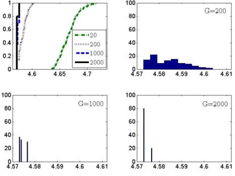
An illustration on the distribution of resulting IC values for 100 Monte-Carlo restarts (𝑛 = 400, 𝑘 = 50 with only five of them actually involved in generating an artificial response variable) can be found in Figure 1. In-creasing 𝐺 the distribution shifts left and becomes less dispersed (see also Gilli and Winker (2009, page 98)). Since GA are a stochastic method, the algorithm is restarted ten times and the solution with the best IC value is selected.
3
Monte-Carlo study
In this Section the performance of the Lasso-type methods (Lasso, aLasso, EN) and the one of the subset-selection technique via GA (BIC, HQIC) are compared. The goal of this comparison is to determine how stable the methods are: in what Monte-Carlo set-ups each of them provides superior results (in terms of correctly identified subsets and estimation accuracy) and what is the corresponding CPU time needed.
The Monte-Carlo set-ups below have certain parallels with the scenarios tested in Frank and Friedman (1993), Zou (2006) and Zou and Zhang (2009), making potential comparison of the results possible. However, there are also significant distinctions in the DGP (e.g., amount of noise, portion of relevant regressors) and in the scope of the methods tested (including both the Lasso-type and the heuristic model selection methods).
3.1
Data generating process
In order to compare the performance of the Lasso-type techniques with the GA algorithm implemented, various artificial data sets are generated. These set-ups are tested using different numbers of regressors in a data set and different numbers of observations per regressor (𝑘 = 50 and 𝑛 = 400, 𝑘 = 50 and 𝑛 = 100 or 𝑘 = 100 and 𝑛 = 60). In the latter case the situation where 𝑘 ≫𝑛 is analyzed.
The covariance matrix Σ is set either Σ𝑖,𝑗 = 0.5∣𝑖−𝑗∣ or 0.75∣𝑖−𝑗∣ with
1 ≤𝑖, 𝑗 ≤𝑘. In the former case, all off-diagonal elements do not exceed 0.5 (’low correlation’); in the latter one, pairwise highly correlated regressors are generated (’high correlation’). The ’true’ regression coefficient vector (𝛽𝑚𝑐)
contains either a small or a large portion of non-zero coefficients (𝑘𝑡𝑟𝑢𝑒 =
5or25, respectively), which are either equal (𝛽𝑚𝑐
𝑗 = 1) or unequal (𝛽𝑗𝑚𝑐=𝑗2).
In the latter case 𝛽𝑗𝑚𝑐 = (1,4,9,16, ...).
For each set-up, 50 restarts of the following procedure are performed. First, a set of regressors (𝑋𝑚𝑐) with a joint Gaussian distribution and a specified Σ is randomly generated. Then, using 𝛽𝑚𝑐 and adding an i.i.d. error term, the response variable (𝑦𝑚𝑐) is generated as follows:
𝑦𝑚𝑐 =𝑋𝑚𝑐𝛽𝑚𝑐+𝜀, 𝜀∼𝑛(0, 𝜎2𝜀), (20) where 𝜎𝜀2 is the variance of the residuals.
In (20) one chooses 𝜎 such that the corresponding signal-to-noise ratio (SNR) is either 5 (’low noise’) or 0.5 (’high noise’), where the SNR is given by:
SNR= (var(𝑋
𝑚𝑐𝛽𝑚𝑐))1/2
𝜎 . (21)
3.2
Simulation results
The simulation results are compared using the True Positive Rate (TPR) and the False Negative Rate (FNR)5 as estimations of a correctly identified
model. The mean-squared error (MSE = 𝐸[(𝛽ˆ− 𝛽𝑚𝑐)′Σ(𝛽ˆ−𝛽𝑚𝑐)]) with standard deviations computed over 50 replications given in parentheses are used as a measure of the estimation accuracy. In addition, the CPU time corresponding to a single restart using Matlab 7.7 on a Pentium IV 2.67 GHz is reported.6
As one can see in Table 1, Lasso-type solutions perform well identifying the correct subset structure in the scenario with low level of noise7 (at most, only one false regressor included). It is also clear that in the case of high correlation and low noise level, EN outperforms other Lasso-type methods.
However, in the scenario with high amount of noise, all Lasso-type meth-ods tend to exclude two or three ’true’ regressors from the solution identified (FNR≈4-6%). In this case aLasso performs the best out of the other Lasso-type techniques.8 If the regressors in the ’true’ subset are also correlated, some false regressors are selected by all of the Lasso-type estimators. This 5TPR is the percentage of ’true’ regressors from all variables selected and FNR is the portion of rejected ’true’ regressors among correctly selected and correctly rejected ones.
6For each of the methods, the averaged results over 50 replications of the procedure are reported.
7This corresponds to the situation when a data set includes the majority of significant predictors which explain𝑦.
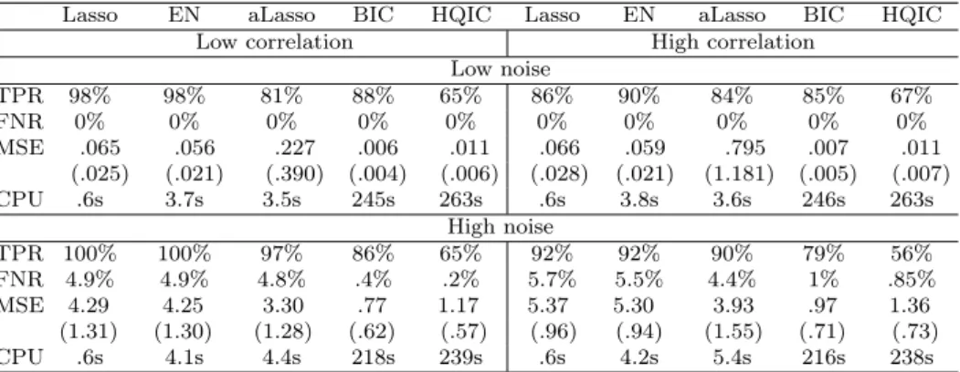
Table 1: Simulation results for𝑛 = 400, 𝑘= 50, 𝑘𝑡𝑟𝑢𝑒 = 5 and 𝛽𝑗𝑚𝑐= 1.
Lasso EN aLasso BIC HQIC Lasso EN aLasso BIC HQIC
Low correlation High correlation
Low noise TPR 98% 98% 81% 88% 65% 86% 90% 84% 85% 67% FNR 0% 0% 0% 0% 0% 0% 0% 0% 0% 0% MSE .065 .056 .227 .006 .011 .066 .059 .795 .007 .011 (.025) (.021) (.390) (.004) (.006) (.028) (.021) (1.181) (.005) (.007) CPU .6s 3.7s 3.5s 245s 263s .6s 3.8s 3.6s 246s 263s High noise TPR 100% 100% 97% 86% 65% 92% 92% 90% 79% 56% FNR 4.9% 4.9% 4.8% .4% .2% 5.7% 5.5% 4.4% 1% .85% MSE 4.29 4.25 3.30 .77 1.17 5.37 5.30 3.93 .97 1.36 (1.31) (1.30) (1.28) (.62) (.57) (.96) (.94) (1.55) (.71) (.73) CPU .6s 4.1s 4.4s 218s 239s .6s 4.2s 5.4s 216s 238s
results in a large estimation bias.
In contrast, the results of the heuristic method are not influenced as strongly by the amount of noise in the simulated data sets. In terms of the estimation bias IC via heuristics outperform all Lasso-type solutions in both set-ups with low and high SNR. This is most obvious with the Bayesian IC that provides sparser models in comparison to HQIC. To this end, for small SNR IC via heuristics are better off identifying the ’true’ subset (on average, BIC includes or excludes not more than one variable incorrectly).
In terms of the CPU time, the Lasso-type methods have a significant advantage over the heuristic approach. As an example, one Lasso simulation does not last longer than 1s. Since EN and aLasso require a two-dimensional cross-validation, they need 3-5s on average. IC via GA need about 250s per restart for 𝑛 = 400. Reducing 𝑛 results in a corresponding decline in the CPU time.
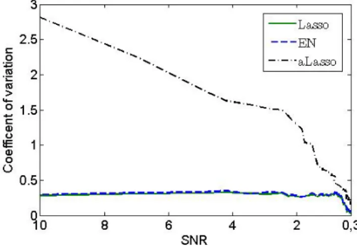
In Table 1 the high variance in the estimated bias for aLasso (especially, in the situation with low noise level) is remarkable. In an additional experiment the described set-up is simulated 100 times for SNR∈(0.3,10) and the coef-ficient of variation for all three Lasso-type solutions is measured (Figure 2). Obviously, for SNR >0.5 the variation in results for aLasso is much higher than for other Lasso-type methods. Similar results can be obtained for both
ridge- and OLS-weighths and are present in all our simulation studies.9
Figure 2: Coefficients of variation for Lasso-type estimators.
In the following one or two characteristics in the simulation set-up psented in Table 1 are changed and only major differences in results are re-ported. Thus, considering different regression coefficients (Table 2), one can see that the relative supremacy of the heuristic approach has remained. All methods tested under this scenario exclude more correct regressors, which results in a higher MSE.
Increasing the portion of ’true’ regressors (𝑘𝑡𝑟𝑢𝑒 = 25), one finds that
for high SNR heuristics outperform the Lasso-type methods in identifying the correct subset structure (Table 3). There can be two reasons for this. First, due to the stronger parsimony property of the Lasso methods (aLasso excludes correct variables even with the small portion of noise). Second, due to the larger proportion of relevant predictors, the problem of correlated predictors is more challenging. This is evident when one compares the left and the right panels of Table 3. Reducing the SNR leads to a much larger proportion of mistakes in model selection for all methods. Nevertheless, the
9This is mainly due to the asymptotic property of the aLasso-weights ( ˆ
𝜔𝑗) adding some
instability in the model estimation. For SNR>0.5and, respectively, smaller MSE values this instability becomes more evident.
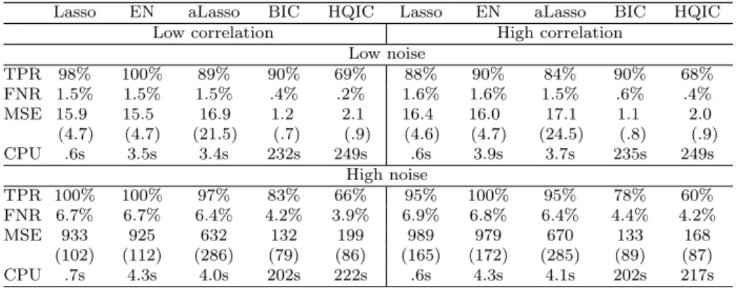
Table 2: Simulation results for𝑛 = 400,𝑘 = 50, 𝑘𝑡𝑟𝑢𝑒= 5 and 𝛽𝑚𝑐 𝑗 =𝑗2.
Lasso EN aLasso BIC HQIC Lasso EN aLasso BIC HQIC
Low correlation High correlation
Low noise TPR 98% 100% 89% 90% 69% 88% 90% 84% 90% 68% FNR 1.5% 1.5% 1.5% .4% .2% 1.6% 1.6% 1.5% .6% .4% MSE 15.9 15.5 16.9 1.2 2.1 16.4 16.0 17.1 1.1 2.0 (4.7) (4.7) (21.5) (.7) (.9) (4.6) (4.7) (24.5) (.8) (.9) CPU .6s 3.5s 3.4s 232s 249s .6s 3.9s 3.7s 235s 249s High noise TPR 100% 100% 97% 83% 66% 95% 100% 95% 78% 60% FNR 6.7% 6.7% 6.4% 4.2% 3.9% 6.9% 6.8% 6.4% 4.4% 4.2% MSE 933 925 632 132 199 989 979 670 133 168 (102) (112) (286) (79) (86) (165) (172) (285) (89) (87) CPU .7s 4.3s 4.0s 202s 222s .6s 4.3s 4.1s 202s 217s
heuristic approach still results in a lower MSE.10
Table 3: Simulation results for 𝑛= 400, 𝑘 = 50, 𝑘𝑡𝑟𝑢𝑒= 25 and 𝛽𝑚𝑐 𝑗 = 1.
Lasso EN aLasso BIC HQIC Lasso EN aLasso BIC HQIC
Low correlation High correlation
Low noise TPR 83% 84% 98% 98% 92% 76% 77% 98% 97% 90% FNR 0% 0% .9% 0% 0% 0% 0% 2.3% 0% 0% MSE .58 .57 3.34 .11 .15 .65 .64 5.26 .14 .19 (.09) (.08) (5.61) (.04) (.03) (.16) (.15) (10.3) (.04) (.03) CPU .5s 2.9s 2.5s 428s 452s .5s 3.3s 2.5s 434s 464s High noise TPR 91% 91% 87% 83% 75% 71% 71% 72% 72% 70% FNR 24% 24% 23% 21% 19% 21% 21% 24% 22% 21% MSE 41.3 41.2 37.9 28.3 25.2 45.0 44.7 58.7 26.9 24.1 (2.4) (2.4) (2.9) (2.4) (2.9) (6.7) (6.7) (7.0) (6.2) (3.9) CPU .6s 4.1s 3.7s 244s 284s .7s 4.1s 4.4s 246s 275s
If one reduces the sample size (𝑛 = 100), the Lasso-type methods (except aLasso) are less affected by the asymptotic property than IC via heuristics (Table 4). In the case of low level of noise, heuristics are still better off in terms of MSE, although they accept significantly more false regressors. But for high noise level Lasso-type methods surpass IC via GA in terms of the estimation bias.11 In general, this is good evidence that Lasso are more 10Due to the higher 𝑘𝑡𝑟𝑢𝑒, the heuristic requires more CPU time (approximately 450s)
identifying all ’true’ predictors under low noise and estimating their regression coefficients. 11An exception is constituted for the case with correlated predictors: since the Lasso
suitable for small 𝑛 (see also Hsu et al. (2007, page 3649)).
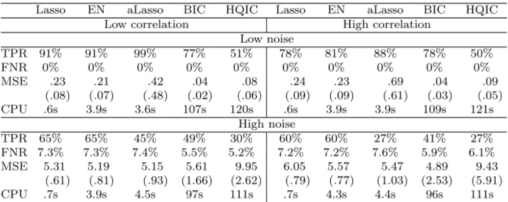
Table 4: Simulation results for𝑛 = 100, 𝑘= 50, 𝑘𝑡𝑟𝑢𝑒 = 5 and 𝛽𝑚𝑐 𝑗 = 1.
Lasso EN aLasso BIC HQIC Lasso EN aLasso BIC HQIC
Low correlation High correlation
Low noise TPR 91% 91% 99% 77% 51% 78% 81% 88% 78% 50% FNR 0% 0% 0% 0% 0% 0% 0% 0% 0% 0% MSE .23 .21 .42 .04 .08 .24 .23 .69 .04 .09 (.08) (.07) (.48) (.02) (.06) (.09) (.09) (.61) (.03) (.05) CPU .6s 3.9s 3.6s 107s 120s .6s 3.9s 3.9s 109s 121s High noise TPR 65% 65% 45% 49% 30% 60% 60% 27% 41% 27% FNR 7.3% 7.3% 7.4% 5.5% 5.2% 7.2% 7.2% 7.6% 5.9% 6.1% MSE 5.31 5.19 5.15 5.61 9.95 6.05 5.57 5.47 4.89 9.43 (.61) (.81) (.93) (1.66) (2.62) (.79) (.77) (1.03) (2.53) (5.91) CPU .7s 3.9s 4.5s 97s 111s .7s 4.3s 4.4s 96s 111s
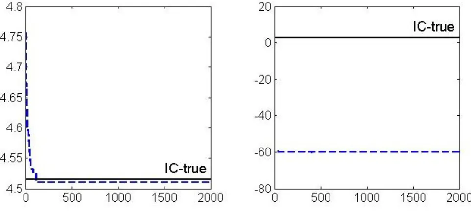
Finally, considering an overdetermined linear system one finds that the performance of all methods dramatically decreases (Table 5). This is more evident for the heuristic approach. The case with 𝑘 ≫ 𝑛 can result in extremely small RSS values if a large number of available regressors (𝑘 ∼𝑛) is included. As the IC’s natural logarithm goes to minus infinity, the penalty on model complexity remains in the same (former) order of magnitude. Hence, the resulting difference in IC ’compensates’ incorrect variables to be included by GA.12 An illustration of this effect is presented in Figure 3. In the left plot with 𝑛 = 400, GA identifies a smaller IC value (dashed line) than the one attributed to the ’true’ subset structure (’IC-true’). The smaller the 𝑛, the larger the difference between the two values. In the extreme case with
𝑘 ≫𝑛 (right plot) this difference becomes much more apparent.
Consequently, the real limitation of the heuristic approach is the objective function (18) that is not suitable for 𝑘 ≫ 𝑛, while GA algorithm performs well in both set-ups (for more discussion on this see Appendix). In the set-up with 𝑘 ≫ 𝑛, Lasso-type methods (in particular, Lasso and EN) are superior model selection strategies in terms of both correctly identified subset structures and estimated bias.13
methods are inconsistent here, BIC via GA provides a smaller MSE. 12A similar finding is also made for the Akaike information criterion.
pre-Figure 3: IC values for different sample sizes.
Table 5: Simulation results for𝑛 = 60, 𝑘 = 100, 𝑘𝑡𝑟𝑢𝑒 = 5 and 𝛽𝑚𝑐 𝑗 = 1.
Lasso EN aLasso BIC HQIC Lasso EN aLasso BIC HQIC
Low correlation High correlation
Low noise TPR 61% 75% 49% 8% 8% 43% 54% 46% 8% 8% FNR 0% 0% 0.1% 0% 0% 0% 0% 0.1% 0% 0% MSE .18 .16 .25 1.41 1.81 .16 .15 0.13 1.75 2.11 (.10) (.09) (.87) (.49) (.86) (.09) (.08) (0.51) (1.10) (1.68) CPU 0.7s 5.2s 5.4s 914s 964s 0.7s 5.3s 5.7s 917s 967s High noise TPR 38% 38% 19% 6% 5% 32% 32% 13% 4% 5% FNR 4.2% 4.2% 3.7% 3% 4% 4.2% 4.2% 3.9% 5% 4% MSE 4.99 5.04 13.03 73.08 73.39 5.15 5.15 23.32 79.82 83.88 (.28) (.51) (9.4) (14.05) (16.45) (.25) (.36) (28.78) (17.42) (24.85) CPU .7s 4.8s 4.5s 916s 925s .8s 4.9s 5.4s 1339s 1091s
4
Application on a cross-country growth model
To illustrate the model selection techniques, let us apply them to an actual empirical problem, using the real per capita GDP growth rate over 1960-1992 and a series of country’s characteristics evaluated for 1960.14 The data set was first tested and described in detail by Sala-i-Martin (1997). Due to a large number of missing observations, Fernandez et al. (2001) reduce the original
screening that reduces the dimensionality of the problem is employed in this study (as e.g., Sure Independent Screening). Thus, only the methods described in Section 2 are considered.
14A set of characteristics is selected that best explains the GDP growth rate within a standard linear regression model.
Table 6: Summary results for the cross-country growth model.
BIC BIC(adj.) Lasso EN aLasso Constant 0.0797 0.0419 0.0206 0.0399 0.0998
Primary school enrollment 0.0249 - - - -Life expectancy 0.0009 0.0010 0.0010 0.0009 0.0011
Log of per capita GDP −0.0188 −0.0130 −0.0111 −0.0126 −0.0177
Fraction of confucius 0.0759 0.0577 0.0423 0.0460 -Fraction of muslim 0.0078 0.0118 0.0052 0.0038 -Sub-Saharan dummy −0.0218 - −0.0091 −0.0131 −0.0209 Rule of law 0.0131 - 0.0103 0.0108 0.0096 Equipment investment 0.1511 0.2181 - 0.0036 -... ... ... ... ... ... ℎ=22 ℎ=7 ℎ=32 ℎ=34 ℎ=10 𝑅2(adjusted) 92% 79% 78% 81% 67%
data set from 134 countries and 62 regressors to 72 and 42, respectively. The data was used in a series of studies applying different model selection strategies. The most interesting for us (for comparative reasons) are the ap-plication of genetic algorithms by Acosta-Gonzalez and Fernandez-Rodriguez (2007) and adaptive Lasso by Schneider and Wagner (2009).
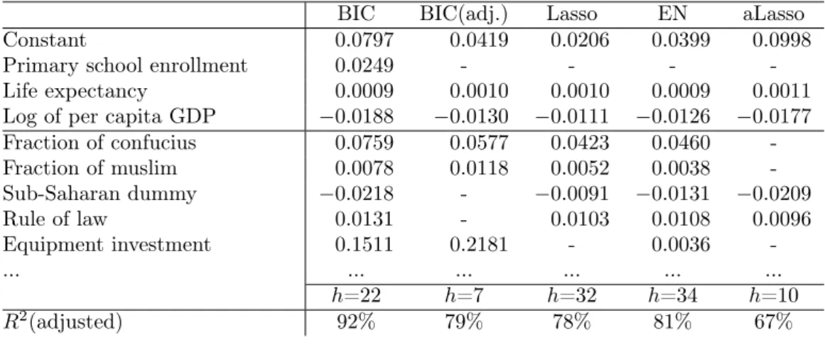
A brief summary of the results for the data set with a total number of regressors included (ℎ) by each strategy is presented in Table 6 (see Table 8 in Appendix for a complete version of the results). As one can see, BIC via GA, Lasso and EN include more than half of the available regressors in the final solution. Comparing their model fits, the IC has the highest 𝑅2 adjusted with the smaller subset of predictors.15 This can be due to a larger
number of incorrect variables included by the Lasso-type methods (see results in Table 3). Based on this and together with our Monte-Carlo simulations, the model estimation obtained via GA is considered as the most accurate one in this particular example. Due to a potentially large portion of relevant regressors and high pairwise correlation between certain variables (e.g., for equipment investment and life expectancy it is above 0.64), EN is seen to outperform the other Lasso-type methods.16
15In contrast, aLasso rather excludes some relevant regressors, which results in the smaller goodness-of-fit.
Acosta-Gonzalez and Fernandez-Rodriguez (2007) try to avoid over-para-metrization with an adjusted BIC (18) by doubling its penalty on model complexity. They come up with a smaller model subset (see BIC(adj.)). By employing Algorithm 2 for GA, the same model as in Acosta-Gonzalez and Fernandez-Rodriguez (2007) is identified.
In Table 8 two out of three regressors always included by Sala-i-Martin (1997) are also selected by all the model selection strategies: life expectancy and GDP per capita. In contrast, there is less evidence for primary school enrollment to be retained in the model. This finding is also supported by Fernandez et al. (2001).
5
Conclusions and outlook
The model specification step has a vital role for the further regression anal-ysis, since any ad-hoc or intuitive decisions can reduce the estimation accu-racy or introduce an estimation bias. In this study the Lasso-type (Lasso, adaptive Lasso, elastic net) and a heuristic model selection strategy are com-pared. First, one describes the implementation of all methods underlining their strengths and weaknesses. Second, an illustration of their performances based on several Monte-Carlo experiments is provided. Finally, the methods are implemented on real empirical data and their results are contrasted.
One finds that an application of the Lasso modifications has some influ-ence on its resulting performance in terms of both subset selection correctness and estimation bias. However, this influence is rather marginal in comparison to other model selection methods, in particular, heuristic optimization.
In general, the Lasso-type techniques provide sparser solutions than the heuristic approach. They can better identify irrelevant predictors in a final subset, but exclude more relevant ones. As a result, in most of the simulated set-ups the Lasso methods exhibit a larger estimation bias. If the portion of relevant regressors in a given data set is large or available regressors can ex-plain the indicator of interest to a large extent (’small noise’), the supremacy
Schneider and Wagner (2009). This is due to another choice of tuning parameters made. In particular, Schneider and Wagner (2009) employ OLS-weights and set𝜐 equal to one.
of the heuristics becomes more apparent.
Based on the simulated experiments, one can consider the Lasso methods more suitable for data sets with small sample sizes. In contrast, application of heuristics in this case is constrained by the asymptotic property of IC.
The Lasso methods have a significant advantage over heuristic methods in terms of the CPU time required. Although, as it is demonstrated in this study, nowadays IC via heuristics can be optimized using reasonable computational time.
In the future one can compare the methods discussed with the adaptive elastic net (Zou and Zhang 2009) that combines strengths of the elastic net and the adaptive lasso, or with the adaptive ridge selector (Armagan and Zaretzki forthcoming) that differentiates amounts of shrinkage according to t-statistics. An alternative is to test an application of heuristic methods on the generalized 𝐿𝑞-norm approach with 0< 𝑞 <1.
Acknowledgements Valuable comments and suggestions from Peter Winker, Thomas Wagner, Marianna Lyra and Henning Fischer are gratefully acknowl-edged. All remaining shortcomings are my responsibility.
References
Acosta-Gonzalez, E. and F. Fernandez-Rodriguez (2007). Model selction via genetic algorithms illustrated with cross-country growth data.Empirical Economics 33(2), 313–337.
Armagan, A. and R. L. Zaretzki (forthcoming). Model selection via adaptive shrinkage with t priors. Computational Statistics.
Breiman, L. (2001). Statistical modelling: the two cultures. Statistical Sci-ence 16(3), 199–231.
Caner, M. (2009). Lasso-type GMM estimator.Econometric Theory25, 270– 290.
Efron, B., T. Hastie, I. Johnstone and R. Tibshirani (2004). Least angle regression. Annals of Statistics 32, 407–489.
Fan, J. and J. Lv (2008). Sure independence screening for ultrahigh di-mensional feature space. Journal of the Royal Statistical Society B
70(5), 849–911.
Fernandez, C., E. Ley and M. Steel (2001). Model uncertainty in cross-country growth regressions. Journal of Applied Econometrics 16, 563– 576.
Fogel, D. B. (2006). Evolutionary Computation: Toward a New Philosophy of Machine Intelligence. Wiley-IEEE Press. Hoboken, NJ.
Foster, S. D., A. P. Verbyla and W. S. Pitchford (2008). A random model approach for the lasso. Computational Statistics 23, 217–233.
Frank, I. E. and J. H. Friedman (1993). A statistical view of some chemo-metrics regression tools. Technometrics 35(2), 109–135.
Gilli, M. and P. Winker (2009). Heuristic optimization methods in economet-rics. In: Handbook of Computational Econometrics (D. A. Belsley and E. Kontoghiorghes, Eds.). pp. 81–119. Wiley. Chichester.
Hastie, T., R. Tibshirani and J. Friedman (2009).The Elements of Statistical Learning: Data Mining, Inference, and Prediction. Springer Verlag. New York.
Hendry, D. F. and H. M. Krolzig (2005). The properties of automatic "GETS" modelling. The Economic Journal 115(502), C32–C61.
Hsu, N.-J., H.-L. Hung and Y.-M. Chang (2007). Subset selection for vector autoregressive processes using lasso. Computational Statistics & Data Analysis 52(7), 3645–3657.
Johnson, B. A. (2009). On lasso for censored data. Electronic Journal of statistics 3, 485–506.
Knight, K. and W. Fu (2000). Asymptotics for lasso-type estimators.Annals of Statistics 28(5), 1356–1378.
Maringer, D. and P. Winker (2009). The convergence of estimators based on heuristics: Theory and application to a GARCH model. Computational Statistics 24, 533–550.
Perez-Amaral, T., G. M. Gallo and H. White (2003). A flexible tool for model building: The relevant transformation of the inputs network approach (RETINA).Oxford Bulletin of Economics and Statistics65(1), 821–838.
Sala-i-Martin, X. (1997). I just ran four million regressions. Technical Report 6252. NBER Working Paper.
Savin, I. and P. Winker (2010). Heuristic optimization methods for dynamic panel data model selection. Application on the Russian innovative per-formance. Technical Report 27. COMISEF Working Papers Series. Schneider, U. and M. Wagner (2009). Catching growth determinants with
the adaptive lasso. Technical Report 55. wiiw Working Paper.
Sin, C.-Y. and H. White (1996). Information criteria for selecting possibly misspecified parametric models. Journal of Econometrics71(1-2), 207– 225.
Tibshirani, R. (1996). Regression shrinkage and selection via the lasso. Jour-nal of the Royal Statistical Society B 58(1), 267–288.
Winker, P. (1995). Identification of multivariate AR-models by threshold accepting. Computational Statistics & Data Analysis 20(3), 295–307. Zhao, P. and B. Yu (2006). On model selection consistency of lasso. Journal
of Machine Learning Research 7, 2541–2563.
Zou, H. (2006). The adaptive lasso and its oracle properties. Journal of the American Statistical Association 101, 1418–1429.
Zou, H. and H. H. Zhang (2009). On the adaptive elastic-net with a diverging number of parameters. Annals of Statistics 37(4), 1733–1751.
Zou, H. and T. Hastie (2005). Regularization and variable selection via the elastic net. Journal of the Royal Statistical Society B 67(2), 301–320.
6
Appendix
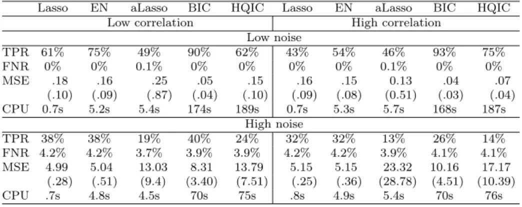
Extensively simulating with different forms of IC (with absolute values of the logarithm and the use of RSS’s absolute value instead of its logarithm in conjunction with a re-scaled penalty for model complexity) one can find an ’adjusted’ IC form suitable for the 𝑘 ≫ 𝑛 case. For example, one can take RSS absolute value and adjust the penalty term via a data-driven multipli-cator 𝜅 set equal to 20 or 1600 (depending on the SNR):
IC=∥𝑦−𝑋𝛽ˆ∥22 +𝜅ℎln(𝑛)/𝑛, (22) In the result, one can obtain much better results for the IC via GA (Ta-ble 7). However, this form of the IC is no longer ’universal’ and has to be calibrated for each particular data set.
Table 7: Simulation results for𝑛 = 60, 𝑘 = 100, 𝑘𝑡𝑟𝑢𝑒 = 5 and 𝛽𝑚𝑐 𝑗 = 1.
Lasso EN aLasso BIC HQIC Lasso EN aLasso BIC HQIC
Low correlation High correlation
Low noise TPR 61% 75% 49% 90% 62% 43% 54% 46% 93% 75% FNR 0% 0% 0.1% 0% 0% 0% 0% 0.1% 0% 0% MSE .18 .16 .25 .05 .15 .16 .15 0.13 .04 .07 (.10) (.09) (.87) (.04) (.10) (.09) (.08) (0.51) (.03) (.04) CPU 0.7s 5.2s 5.4s 174s 189s 0.7s 5.3s 5.7s 168s 187s High noise TPR 38% 38% 19% 40% 24% 32% 32% 13% 26% 14% FNR 4.2% 4.2% 3.7% 3.9% 3.9% 4.2% 4.2% 3.9% 4.1% 4.1% MSE 4.99 5.04 13.03 8.31 13.79 5.15 5.15 23.32 10.16 17.17 (.28) (.51) (9.4) (3.40) (7.51) (.25) (.36) (28.78) (4.51) (10.39) CPU .7s 4.8s 4.5s 70s 75s .8s 4.9s 5.4s 70s 76s
Table 8: Results for the cross-country growth model.
BIC BIC(adj.) Lasso EN aLasso
Constant 0.0797 0.0419 0.0206 0.0399 0.0998
Primary school enrollment 0.0249 - - -
-Life expectancy 0.0009 0.0010 0.0010 0.0009 0.0011
Log of per capita GDP -0.0188 -0.0130 -0.0111 -0.0126 -0.0177
Fraction of GDP in mining 0.0328 - 0.0337 0.0370
-Degree of capitalism - - 0.0023 0.0022
-Number of years open economy - 0.0176 0.0056 0.0036
-Fraction speaking English -0.0078 - -0.0058 -0.0064
-Fraction speaking foreign language - - -0.0008 -0.0006
-Exchange rate distortions - - 3.3×10⁻⁶ 2.4×10⁻⁶
-Equipment investment 0.1511 0.2181 - 0.0036
-Non-equipment investment 0.0295 - 0.0108 0.0256
-Std dev of black market premium - - −2.4×10⁻⁶ −1.8×10⁻⁶
-Outward orientation -0.0035 - -0.0021 -0.0023
-Black market premium -0.0055 - -0.0037 -0.0041
-Total area of the country - - −2.5×10⁻⁸ −3.3×10⁻⁸ 6.1×10⁻¹⁰
Latin American dummy -0.0127 - -0.0050 -0.0055 -0.0118
Sub-Saharan dummy -0.0218 - -0.0091 -0.0131 -0.0209
Higher education enrollment -0.1213 - - -
-Public education share - - - -
-Revolutions and coups - - 0.0012 0.0012
-War dummy - - -0.0024 -0.0033
-Political rights - - -0.0016 -0.0019
-Civil liberties -0.0028 - 0.0019 0.0017 -0.0016
Absolute latitude - - −3.6×10⁻⁷ −1.6×10⁻⁶ −4.4×10⁻⁶
Average age of the population - - −5.0×10⁻⁶ −4.5×10⁻⁶
-British colony dummy 0.0079 - 0.0011 0.0015
-Fraction of buddhist - - 0.0140 0.0121
-Fraction of catholic - - -0.0014 -0.0024
-Fraction of confucius 0.0759 0.0577 0.0423 0.0460
-Ethnolinguistic fractionalization 0.0165 - - 0.0019
-French colony dummy 0.0110 - - -
-Fraction of hindu -0.1108 - -0.0051 -0.0263 -0.0017 Fraction of jewish - - - - -Fraction of muslim 0.0078 0.0118 0.0052 0.0038 -Primary exports - - -0.0039 -0.0040 -Fraction of protestant - -0.0136 -0.0108 -0.0111 -Rule of law 0.0131 - 0.0103 0.0108 0.0096
Spanish colony dummy 0.0140 - - -
-Growth rate of population - - - -
-Ratio workers to population - - -0.0126 -0.0113
-Labor force −3.8×10⁻⁸ - 2.6×10⁻⁹ 7.9×10⁻⁹ −4.9×10⁻⁹
𝑅2 95% 81% 88% 91% 72%