4766.pdf

Housing Wealth Effects Mechanism and the Monetary Policy Transmission in

Turkey

Mustafa Haluk Guler

A dissertation submitted to the faculty of the University of North Carolina at Chapel

Hill in partial fulfillment of the requirements for the degree of Doctor of Philosophy in

the Department of Economics.

Chapel Hill

2012

Approved by:

Richard T. Froyen

Neville R. Francis

Lutz A. Hendricks

Jonathan B. Hill

c

2012

Abstract

Mustafa Haluk Guler: Housing Wealth Effects Mechanism and the Monetary Policy

Transmission in Turkey

(Under the direction of Richard T. Froyen)

It is commonly presumed that significant movements in wealth can often have wider

eco-nomic impacts in consumer spending. This study first investigates the impact of

hous-ing wealth on aggregate consumer spendhous-ing in the context of Turkey ushous-ing a Vector

Er-ror Correction Method (VECM) under the structural break with quarterly data for the

1991Q1-2011Q1 period. Furthermore, to improve the robustness to instability in the

long-run relationship between the variables, we also estimate an alternative econometric

model based upon Carroll (2004). Both the VECM and Carroll’s method suggest that

permanent changes in housing wealth have considerable effects on aggregate

consump-tion after 2001 while there is no significant financial wealth effect for the same period.

Since our VECM results indicate that housing wealth does play a role in determining

consumption, the next step is to find out whether there is a linkage between monetary

policy and housing wealth and if so, how this relationship operates. For this purpose,

we employ a kind of counterfactual experiment. Our results show that interest rate

af-fects the housing market considerably and house prices play an important role in the

Acknowledgments

I would like to express my sincere gratitude to a number of people who provided valuable

assistance and support through my academic journey.

First, I wish to express my appreciation to Dr. Richard Froyen, my committee

chair-man and advisor. Throughout the period I have been writing my dissertation, he has

provided very valuable advice and support.

Second, I would like to thank Drs. Lutz Hendricks, Neville Francis and Jonathan

Hill for providing me the benefit of all their experience in guiding my research.

Finally, my sincere gratitude goes out to my friend M. Aykut Attar for his

Table of Contents

List of Tables . . . .

ix

List of Figures . . . .

x

Chapters

1 Introduction . . . .

1

2 Wealth Effects on Consumption: An Empirical Study on Turkey . . . .

6

2.1 Wealth Effects: Housing Wealth and Financial Wealth . . . .

7

2.2 Theoretical Background . . . .

9

2.3 Estimation Methodology . . . 12

2.3.1

Johansen (1988) Estimation Procedure . . . 13

2.3.2

Estimation of the Cointegrating Vector under the Structural Break 15

2.4 Empirical Literature on Turkey . . . 18

2.5 Empirical Analysis . . . 21

2.5.1

Background of Turkish Economy . . . 21

2.5.2

Data . . . 26

2.5.3

Testing for Cointegration . . . 27

2.5.4

Estimation Results . . . 29

2.6 An Alternative Approach to Estimate Welfare Effects . . . 31

2.6.2

Carroll’s Method with Structural Break . . . 35

2.6.3

Estimation Results for Turkey Using Carroll’s Method . . . 36

2.7 Conclusion . . . 37

3 House Prices and the Monetary Policy Transmission in Turkey . . . 39

3.1 MTM and the Role of Housing Prices in the Economy . . . 42

3.2 Review of the Empirical Studies . . . 44

3.2.1

Housing Prices-Interest Rate Linkage . . . 45

3.2.2

Housing Prices-Consumption and Residential Investment Linkage

46

3.2.3

House Prices and MTM . . . 47

3.3 Model . . . 49

3.4 Estimation Methodology . . . 49

3.5 Data and Their Properties . . . 50

3.5.1

Data . . . 50

3.5.2

Testing for Cointegration . . . 51

3.6 Estimation . . . 52

3.6.1

Identification of the Structural Shocks . . . 53

3.6.2

Impulse Responses and Counterfactual Experiment . . . 54

3.7 Results. . . 56

3.7.1

Results of Benchmark Model . . . 56

3.7.2

Counterfactual Experiment . . . 58

3.7.3

Robustness . . . 59

3.8 Conclusion . . . 60

4 Conclusion . . . 62

Appendix A Tables . . . 64

Appendix C Data Sources . . . 106

List of Tables

Table A.1 Annual % Change in Real House Prices for Some Countries . . . 64

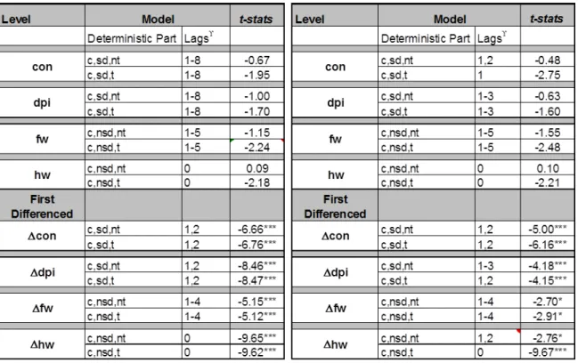
Table A.2 Unit Root Tests (Chap. 2) . . . 65

Table A.3 Information Criteria (Chap. 2) . . . 66

Table A.4 Cointegration Test Results (Chap. 2). . . 67

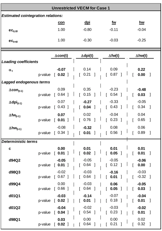
Table A.5 VECM Results for Case 1 . . . 68

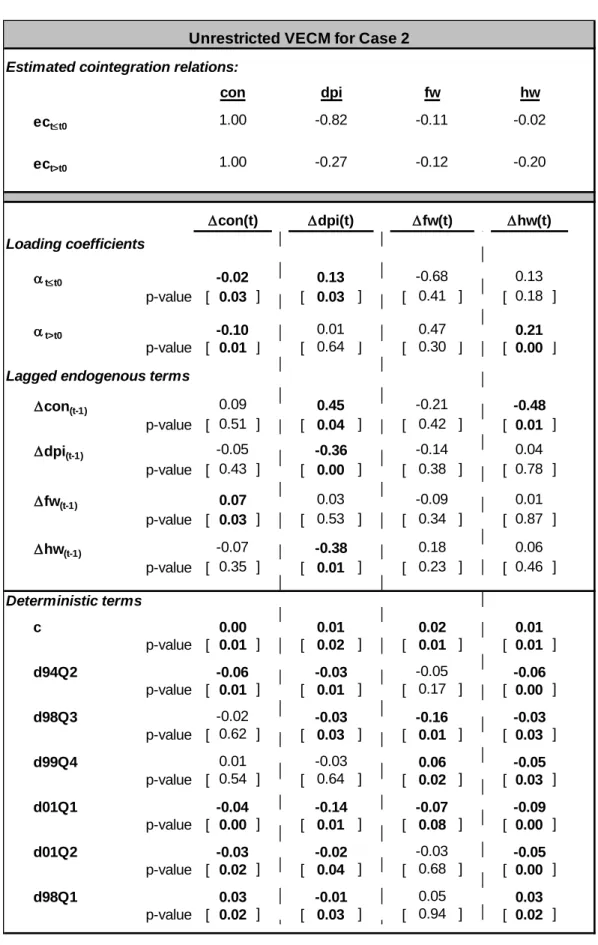
Table A.6 VECM Results for Case 2 . . . 69

Table A.7 LR Tests for Case 1. . . 70

Table A.8 LR Tests for Case 2. . . 71

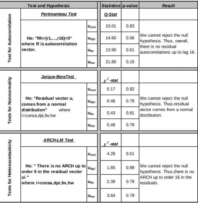
Table A.9 Diagnostic Test Results for Case 1 (Chap. 2) . . . 72

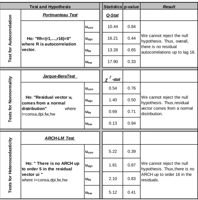
Table A.10 Diagnostic Test Results for Case 2 (Chap. 2) . . . 73

Table A.11 Restricted Cointegration Vectors for Case 1 (Chap. 2) . . . 74

Table A.12 Restricted Cointegration Vectors for Case 2 (Chap. 2) . . . 74

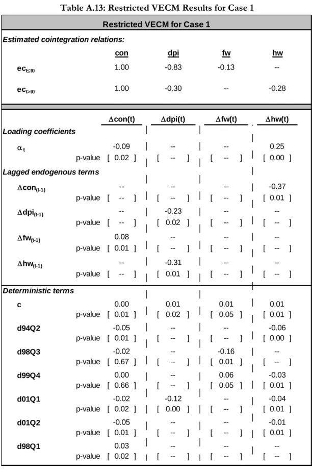
Table A.13 Restricted VECM Results for Case 1 . . . 75

Table A.14 Restricted VECM Results for Case 2 . . . 76

Table A.15 Diagnostic Test Results for Case 1 (Restricted) . . . 77

Table A.16 Diagnostic Test Results for Case 2 (Restricted) . . . 78

Table A.17 Unit Root Tests (Chap. 3) . . . 79

Table A.18 Information Criteria (Chap. 3) . . . 80

Table A.19 Cointegration Test Results (Chap. 3). . . 81

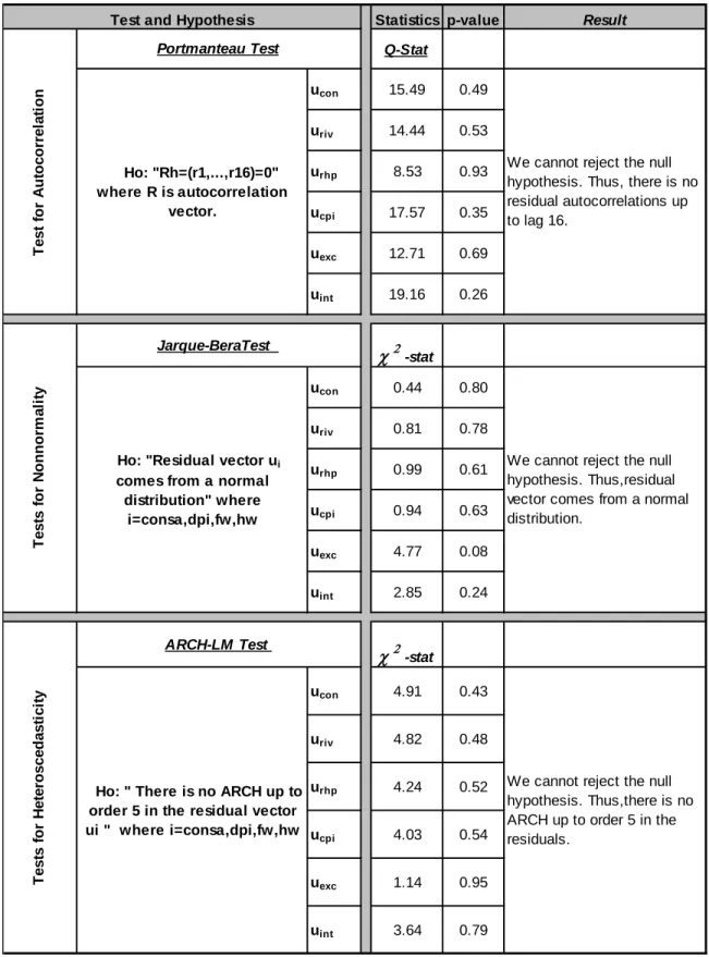
Table A.20 Diagnostic Test Results (Chap. 3) . . . 82

List of Figures

Figure B.1 Ratio of Consumer Credit with Housing Collateral to Total . . . 84

Figure B.2 The Comparison of Real Floor Cost and Real Rent . . . 85

Figure B.3 The Comparison of House Price and Rent . . . 85

Figure B.4 Time-Series Data (Chap. 2) . . . 86

Figure B.5 Monetary Transmission Mechanism . . . 88

Figure B.6 Time-Series Data (Chap. 3) . . . 89

Figure B.7 IRFs for Int. Rate Shock (Benchmark Ordering, pre-2001) . . . 91

Figure B.8 IRFs for Int. Rate Shock (Benchmark Ordering, post-2001) . . . 92

Figure B.9 IRFs for Int. Rate Shock (Benchmark Ordering, 1991-2011) . . . 93

Figure B.10 IRFs for House Price Shock (Benchmark Ordering, pre-2001). . . 94

Figure B.11 IRFs for House Price Shock (Benchmark Ordering, post-2001). . . 95

Figure B.12 IRFs for Int. Rate Shock (Counterfactual Exp., Bench. Ord., pre-2001). 96

Figure B.13 IRFs for Int. Rate Shock (Counterfactual Exp., Bench. Ord., post-2001) 97

Figure B.14 IRFs for Int. Rate Shock (Alternative Ordering 1, pre-2001) . . . 98

Figure B.15 IRFs for Int. Rate Shock (Alternative Ordering 1, post-2001) . . . 99

Figure B.16 IRFs for Int. Rate Shock (Counterfactual Exp., Alt. Ord. 1, pre-2001) . 100

Figure B.17 IRFs for Int. Rate Shock (Counterfactual Exp., Alt. Ord. 1, post-2001) 101

Figure B.18 IRFs for Int. Rate Shock (Alternative Ordering 2, pre-2001) . . . 102

Figure B.19 IRFs for Int. Rate Shock (Alternative Ordering 2, post-2001) . . . 103

Figure B.20 IRFs for Int. Rate Shock (Counterfactual Exp., Alt. Ord. 2, pre-2001) . 104

Chapter 1

Introduction

Household consumption is a function of not only income but also wealth, such as

hous-ing and stock ownership. When the prices of houses or financial assets increase, the

own-ers’ wealth increases and this can spur aggregate consumption, even as income remains

the same. Such change in consumption due to a change in housing or stock prices is called

‘wealth effect’.

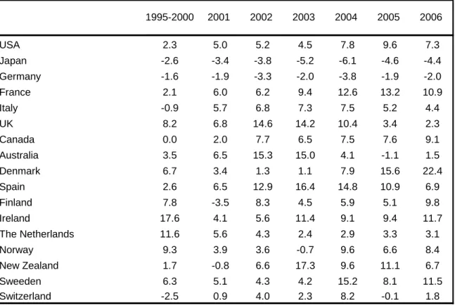
With respect to the wealth effect of housing, the last decade has witnessed dramatic

rise in house prices, followed by substantial price collapse. From 1995-2006, housing

wealth soared globally, with an acceleration after 2000 supported by the combination

of lower interest rates and abundant liquidity. Between the mid 1990s and 2006, the

growth rate of real house price rises in many mature economies reached double-digit

figures (Table A.1).

As the favorable conditions for housing ended with the tightening of monetary policy

in response to global inflationary pressures, housing markets, especially the subprime

mortgage market in the US, came under severe stress. Combined with deficiencies in

the mortgage industry, house prices started to fall dramatically. As measured by the

Standard & Poor’s Case-Shiller index, average home prices in the U.S. were down 32.2

percent as of March 2009 after a peak in the second quarter of 2006. As the subprime crisis

intensified in the US, it damaged the broader economy and eventually triggered a

global output contracted worst since the Great Depression (G-20 Progress Report, 2009).

Since consumption is inherently connected with households’ saving decisions which

could affect price levels and output, in the light of the recent global developments in

housing, it is vital for monetary authority to understand the relationship between

hous-ing wealth and consumption as well as the channels through which such a link might

operate.

Overview of Selected International Studies

There have been numerous academic and government researches that examine

hous-ing wealth effects, particularly for advanced economies. Most, but not all, studies indicate

consensus that rising house prices stimulate consumers to spend more than they would

without such price increases (Case et al. (2005), Ludwig and Slok (2004), Girouard and

Blondal (2001), Carroll et al. (2004)). However, the empirical literature is inconclusive

about the estimates of the marginal propensity to consume out of housing wealth. These

estimates vary substantially across studies. The dispersion in the findings with respect

to the magnitude and timing of the wealth effects stems from the use of different types

of consumption and wealth data and

/

or different estimation techniques that are used to

test the wealth effects. The differences may also stem from the unstable nature of wealth

effects over time.

In recent literature, Case et al. (2005) did a pioneering work in assessing the wealth

effects. The study covered measures of housing wealth for both a panel of 14 developed

economies for the period of 1975-1999 and a panel of all US states from 1982 through

1999. The results of the study suggest that housing wealth effect on consumption is

sta-tistically significant and it is rather large compared to financial wealth for both panels of

data. For the US, the estimate of the elasticity of consumption to housing wealth is found

around 0.04-0.06 while for the international panel, it is about 0.11-0.14. The authors

re-port that the estimated effects for the US are substantially stronger after the mid 1980s

Another multi-country study is conducted by Ludwig and Slok (2004) for the IMF

examining a panel of quarterly data from 1960 through 2000 for 16 OECD economies

divided into bank-based (e.g. Germany, Italy) and market-based (e.g. US, UK) credit

market systems. The authors estimated a larger effect of financial wealth than that from

housing wealth with an MPC of about 8 percent which is twice as large as the elasticity of

house prices. However, due to the use of a single equation approach and data deficiencies

for some countries in the data set, the results are cautioned to be at best, tentative.

Among the studies that have found a role for housing wealth, Girouard and Blondal

(2001) also suggest positive effect of housing wealth for the period 1970-1999 for the US,

the UK, Japan, France as well as Canada with MPCs ranging from 0.02 for the US to 0.18

for Canada, whereas the authors found negative effect of housing wealth for Italy.

Considering the potential instabilities in an economic environment, Carroll et al.

(2004) introduces a new methodology based on the sluggishness of aggregate

consump-tion growth to measure wealth effects for shorter period of time. This method

distin-guishes between immediate (next-quarter) and eventual wealth effects. According to

Car-roll et al.(2004)’s estimation of stock and non-stock wealth effects on consumption for the

US through 1960-2003, while ‘immediate’ wealth effects on consumption are very small

with an MPC out of housing wealth around 2 cents, ‘eventual’ effects are much larger

after several quarters with an MPC amounting to 9 cents.

The Case of Turkey

Although there is a wide range of empirical work, the vast majority of empirical

evidence, refers to advanced economies, particularly the US. However, considering the

increasingly deregulated and deepened financial systems, the accelerated aggregate

con-sumption as well as rising property values in emerging economies, extending the existing

literature to assess the inter-relationship between housing and consumption is critically

important.

housing wealth in Turkey is first motivated by the very high rates of homeownership

and the predominance of housing in total household wealth. The earlier experiences of

very high inflation and shallow financial markets have made the housing asset one of the

most preferred forms of wealth accumulation in Turkey. In addition to that, real price

of housing and the housing stock have followed an increasing trend. Between 2001 and

2011, housing wealth increased approximately 10% annually in real terms. Furthermore,

as the country’s macroeconomic environment has become more stable after 2001, there

has been an expansion of financial products including long-term housing credits. More

importantly, there is a growing interest in mortgage lending which led to the passage of

the new Mortgage Law by the Parliament as of 2007. This legislation is expected to

in-crease the share of housing wealth in wealth composition via raising either the housing

stock (home ownership ratio) or housing prices, ceteris paribus. Due to the recent

devel-opments, future housing wealth effects in Turkey are likely to become more pronounced.

However, to our knowledge, there are only a few contributions which study the

Turk-ish case in depth. Employing weak empirical methodologies and bad proxies for housing

asset value which is due to the lack of data on house stocks and house prices, existing

studies on the housing wealth effect has generally produced poor results. Even more

im-portantly, none of the studies take the structural change in Turkish economy during the

2001 crisis into account.

Chapter II of this dissertation aims to improve the deficiencies of the methodologies

employed in earlier studies by using a system approach that takes the structural break

into consideration, namely the Vector Error Correction Model (VECM), and introduces

a new proxy for housing wealth. Examining the effect of housing wealth as well as

finan-cial wealth upon aggregate consumption in Turkey for the period 1991Q1-2011Q1, our

study indicates that disposable income is the major factor that determines consumption

in Turkey in the long run. However the effect of disposable income decreases after the

2001 crisis whereas the long-run consumption effects of housing wealth get stronger in

crisis while it gets insignificant after the crisis. Furthermore, as an alternative to the

coin-tegration approach, we employ Carroll (2004)’s methodology for the post-crisis period

(after 2001) for estimating the short term and medium term wealth effects on

consump-tion, which does not require stability in cointegrating vectors. The results based on

Car-roll (2004)’s method conclude that both in the short term and medium term, income

and housing wealth have sizeable impacts on consumption whereas no significant effect

is found for financial wealth. The findings of the cointegration approach and Carroll’s

methodology are found to be parallel.

Since consumption is affected by housing wealth, as shown for the Turkish case in

Chapter II, and house prices are influenced by interest rates, there is a channel of

mone-tary policy transmission through house prices and it is important to search how this link

operates. In this regard, Chapter III examines such linkage between monetary policy

and housing wealth and to investigate the role of house prices in monetary transmission

mechanism in Turkey for the period 1991Q1-2011Q1. For this purpose, we employ a

kind of counterfactual experiment. The results show that house prices do play a

consid-erable role in consumption and residential investment in only the medium term (2 year

period) before 2001 whereas they play a crucial role in only the long term (five year

pe-riod) after 2001. Our study suggests that before 2001, following a contractionary interest

rate shock, the increase in house prices is responsible for almost all decreases seen in

con-sumption and residential investment in the medium term. During this period, a house

price change has no long-term effects on consumption and residential investment. After

2001, in response to a contractionary interest rate shock, a decrease in house price has

long-term effects accounting for 33 percent of the fall in consumption and 75 percent of

the fall in residential construction.

The final chapter of this dissertation explores the implications of the findings of

Chapter 2

Wealth Effects on Consumption: An Empirical Study on Turkey

It is commonly presumed that significant movements in wealth can often have wide

economic impacts in consumer spending. This chapter examines the effect of

hous-ing wealth and financial wealth upon aggregate consumption in Turkey for the period

1991Q1-2011Q1 by using a system approach, namely the Vector Error Correction Model

(VECM). The study includes the structral break in the model and improves on the

methodologies presented in previous studies which mostly employed Engle-Granger

sin-gle equation estimation. Having reviewed the earlier methods’ deficiencies to measure

housing wealth, this study also introduces a new measure as a proxy for housing wealth.

The results of the paper indicate that disposable income is the major factor determining

consumption in the long run for Turkey. Also, in the long run, consumption effects of

housing wealth and financial wealth are both found to be positive before 2001. After

the 2001 crisis, housing wealth effect gets larger whereas financial wealth effect becomes

insignificant.

This chapter is organized as follows.

Section 1 reviews the possible

wealth-consumption transmission channels and the arguments on the differences between

hous-ing and financial wealth with respect to their consumption effects. Section 2 briefly

re-views the theoretical framework. Section 3 discusses the estimation methodology while

Section 4 summarizes the empirical literature on Turkey. Section 5 and 6 provide the

2.1 Wealth Effects: Housing Wealth and Financial Wealth

In modern literature, deriving from the permanent income hypothesis developed by

Friedman (1957) and the lifecycle model, developed by Modigliani and Ando (1960) and

Ando and Modigliani (1963), consumption theory suggests that the level of household

consumption is a function of permanent income, demographic variables and physical

wealth that includes both housing and financial wealth. As suggested by the standard

life-cycle model, in response to an unexpected increase in the value of a household’s assets

such as stocks or housing value, a household will increase its spending.

This basic idea and theoretical link between wealth and consumption have been

ex-tended in a number of directions to obtain a more realistic view of consumption

behav-ior. In particular, the so-called collateral effect, which implies an increase in borrowing

capacity, is considered to be an important channel through which accumulated wealth

can stimulate consumer spending. Given the asymmetric information about borrowers

that requires them to provide collateral in credit markets, when there is a rise in wealth,

it will increase the value of the collateral. This will potentially leads to more borrowing

to finance extra consumption using the appreciated asset as collateral. In other words, the

increase in financial wealth or housing wealth can lead to higher consumption by

increas-ing the borrowincreas-ing capacity of previously credit-constrained households. This collateral

channel underpins much of the empirical work on the consumption and housing wealth

link for developed countries like the US and the UK where there is easy access to

mort-gage lending and home equity loans. However, this effect is also becoming significant in

emerging countries like Turkey as the mortgage market and relevant financial products

are developing rapidly, which may be interpreted from Figure B.1

.

According to Figure

B.1, the share of consumer credit with housing collateral in total consumer credits has

risen dramatically in recent years. This may show that the collateral effect of housing

wealth has begun to play an increasing role on consumption behavior of households.

the precautionary motive for saving. Households may choose to hold some assets as a

precaution against negative income shocks. However, when households experience an

increase in wealth, this will lead the value of their “buffer-stock” of wealth to rise and

will allow such households to increase their spending.

In the standard life-cycle view, it is argued that housing and financial wealth effects

are about the same in the long-run. However, this argument is being challenged with the

idea that housing and financial wealth may have different implications for spending. One

of the reasons why the effects could differ is that housing wealth is considered less liquid

than financial wealth because of the high transaction costs with trading in the housing

market. As homeowners are less likely to liquidate their houses in response to a house

price increase, the housing wealth effect on consumption tends to be smaller than the

financial wealth effect.

Another key difference results from the bequest motive which is more important for

housing wealth. For many households, homeownership may be an end in itself due to the

physiological value they attach to the housing asset and their intent to leave their houses

as bequests. Such homeowners who plan to live in their house also obtain a service from

their homes in addition to using their housing assets to accumulate wealth. For them,

a rise in the price of their housing assets may make them to feel wealthier, but this is

not automatically followed by a rise in their consumer spending as the implicit cost of

consuming housing has also increased and they still need housing services in the future.

Also, many homeowners usually appear to be reluctant to trade down into less expensive

houses. Furthermore, for those who intend to buy a house or who are renters, there will

be a negative effect on their wealth as a result of rising house prices. The net housing

wealth effect would depend on the relative share of these categories of population and

the relative size of their responses to changes in house prices; thus, housing wealth could

be more ambiguous and potentially weaker as compared to the financial wealth effect.

One other reason for a more modest effect of housing wealth on consumption relative

to that of financial wealth relies on the idea that changes in stock prices more clearly

indicates future increases in a country’s productivity potential whereas a rise in house

prices may be experienced simply due to supply-side constraints which clearly does not

indicate that the overall economy is better off (Mishkin, 2007).

Despite these theoretical arguments which suggest a smaller impact of housing wealth

on consumption, several empirical studies have found greater consumption effects of

housing wealth. One of the reasons behind these findings is the above mentioned

collat-eral effect. Since housing is by far the most important collatcollat-eral asset for most households

due to the more evenly spread homeownership compared to the ownership of financial

assets which is highly concentrated in a certain population segment, housing wealth can

have stronger impacts on consumption. Moreover, as changes in house prices are much

less volatile than changes in stock prices, the housing wealth effect tends to be more

permanent than financial wealth effect; thus, its impact on spending could be relatively

greater.

2.2 Theoretical Background

The key theoretical link between wealth and consumption, the so-called lifecycle model

developed by Ando and Modigliani (1963) suggests that households use their wealth to

keep their consumption in its planned level. However, it is crucial to solve the nature of

the contemporaneous correlation between changes in wealth and consumption in order

to assess the long-run implications of changes in asset prices.

Following Campbell and Mankiw (1989), Lettau-Ludvigson (2001) first formalized

the idea that consumption, income and wealth move together in the long run. They

that if consumption growth and returns on wealth are stationary, then the log

con-sumption, wealth and labor income should be cointegrated. Following Lettau-Ludvigson

(2001), we present the theoretical framework of this cointegration with the accumulation

of wealth equation, in other words the budget constraint:

W

= (

1

+

R

)(

W

−

C

)

(2.1)

where

W

is aggregate wealth,

C

is consumption and

R

is the net return on

ag-gregate wealth. Campbell and Mankiw (1989) showed that if the consumption to wealth

ratio is stationary, taking the first Taylor approximation of this equation gives the

follow-ing;

∆

w

≈

k

+

r

+ (

1

−

1

/

p

)(

c

−

w

)

(2.2)

where lowercase letters denote log variables,

p

=

1

−

exp

(

c

−

w

)

,

k

is a constant and

r

=

log

(

1

+

R

)

. Solving this equation forward, the consumption wealth ratio may be

written as;

c

−

w

=

X

i=1

p

w

(

r

−

∆

c

)

(2.3)

We can also take this term’s conditional expectation and express it as;

c

−

w

=

E

∞

X

p

i=1

(

r

−

∆

c

)

(2.4)

Total wealth can be written as;

W

=

F W

+

Y

+

HW

(2.5)

as a proxy in the literature. Thus, we can approximate the logarithm of wealth as follows:

w

=

γ

f w

+

θ

y

+ (

1

−

γ

−

θ

)

hw

(2.6)

where

γ

,

θ

and

(

1

−

γ

−

θ

)

are respectively the steady state shares of financial wealth

(

F W

/

W

), disposable income (

Y

/

W

) and housing wealth (

HW

/

W

) in total wealth.

Then, return to aggregate wealth can be expressed as

(

1

+

R

) =

γ

(

1

+

R

) +

θ

(

1

+

R

) + (

1

−

γ

−

θ

)(

1

+

R

)

(2.7)

where

RW

is the return of total wealth,

RF W

is the return of financial wealth,

RY

is the return of human wealth and

RHW

is the return of housing wealth. Taking logs of

both sides and linearizing around the means give;

r w

=

γ

r f w

+

θ

r y

+ (

1

−

γ

−

θ

)

r hw

(2.8)

If we insert Equations (2.6) and (2.8) to the Equation (2.4), we get;

c

−

γ

f w

−

θ

y

−

(

1

−

γ

−

θ

)

hw

=

E

∞

X

p

i=1

(

γ

r f w

+

θ

r y

+(

1

−

γ

−

θ

)

r hw

−

∆

c

)

(2.9)

The equation above shows that the consumption to wealth ratio (left hand side of the

equation) is a function of expected returns and expected changes in consumption (right

hand side of the equation). We can assume that consumption growth (

∆

c

) and the real

returns of the wealth components (

r f w

,

r y

and

r hw

) are stationary. Since the

right hand side of the equation is presumed stationary, the consumption to wealth ratio

should also follow a stationary path, in other words, consumption and wealth should be

short run according to the expected changes in the right hand side variables. However,

this equation does not tell us whether consumption or wealth changes in the long run for

the correction of the long run disequilibrium.

2.3 Estimation Methodology

Following Lettau-Ludvigson (2001), recent macroeconomic studies have analyzed the

consumption function using logarithmic approximation of the budget constraint and

searched for the cointegration relationship between consumption, income and wealth

that is shown in Equation (2.9). The steady state share coefficients

γ

and

θ

in the

equa-tion also give the long run elasticities of consumpequa-tion with respect to different forms of

wealth. This in turn helps to derive the marginal propensity from the given values.

In the short run, it is more likely to have some deviations from the long-run

rela-tionship. Thus, the system moves to restore the equilibrium. In order to investigate the

short-run dynamics that include the variables’ adjustments to restore the long run

equi-librium and the time taken in this process, the Engle-Granger single equation estimation

method (ECM) is often used by researchers.

The Engle-Granger approach is applied in two steps. In the first step, the long run

re-lationship is identified. Using this long run rere-lationship in the second step as one of

the regressors, a short run function of one of the endogenous variables is estimated.

In the literature, the Engle-Granger method is used to estimate the consumption

func-tion by assuming that both income and wealth variables are weakly exogenous. In other

words, it is assumed that only consumption is affected from the disequilibrium and it

performs the adjustment while income and wealth do not. However, this is not always

the case and it is also not supported by the theoretical framework (Lettau and Ludvigson,

2001). Equation (2.9) gives no guidance about how the adjustment occurs. If in reality,

than the Engle-Granger method, we should use a framework that allows for the

possibil-ity that any or all variables perform this adjustment. Thus, we assume that all variables

are endogenous and estimate them in a system of equations, namely the VECM.

2.3.1 Johansen (1988) Estimation Procedure

In order to formulate the VECM, first we write the VAR model assuming that the

VAR(m) model only contains

m

endogenous I(1) variables;

y

=

µ

y

+

µ

y

+

...

+

µ

y

+

ǫ

(2.10)

where "

ǫ

"s are unobservable i.i.d. zero mean white noises with

ǫ

∼

(

0,

σ

ǫi t

)

and

Σ

t

=

V

. The model can be reparameterized by subtracting

y

from both sides. By

rearranging them, we get the following VAR model;

∆

y

= Π

y

+ Γ

∆

y

+

....

Γ

∆

y

+

ǫ

(2.11)

where

Π =

p

P

i=1

µ

−

I

and

Γ

=

−

p

P

j=i+1

µ

.

If there are stationary linear combinations of the

m

endogenous non-stationary

vari-ables, in other words, if the non-stationary variables are cointegrated, then;

|

I

−

µ

λ

₋

µ

λ

2

₋

_....

₋

µ

λ

|

=

0

(2.12)

for

λ

=

1. Since the endogenous variables are cointegrated, then the rank(

Π

)

=

r

<

m

,

thus,

Π

can be decomposed as

α

, adjustment coefficients, and

β

, cointegration

coeffi-cients, where both are

mx r

full column rank matrices. Thus, the model can be

reinter-preted as VECM where cointegration relationship

β

y

(error correction term) is one

of the regressors in the system;

The variables in

β

show the long-run relationships among the endogenous variables

whereas

α

measures the impact of deviations from this long-run equilibrium in the short

term.

Π

can be estimated from Equation (2.11) directly by using OLS. However, in order

to estimate the elements of

Π

;

α

and

β

separately, we need to have some identifying

restrictions. In this regard, we follow Johansen (1988, 1991) by using the restrictions that

β

includes eigenvectors, in other words, the cointegrating vectors that are orthogonal to

each other.

In Johansen’s algorithm two set of regressions are estimated;

∆

y

=

Π

+

Π

∆

y

+

Π

∆

y

+

...

+

Π

∆

y

+

u

(2.14)

y

=

Ψ

+

Ψ

∆

y

+

Ψ

∆

y

+

...

+

Ψ

∆

y

+

v

(2.15)

where

Π

and

Ψ

denotes

(

nxn

)

matrices of OLS coefficient estimates. Next step is to

calculate the sample variance-covariance matrices of the OLS residuals

u

and

v

;

ˆ

Σ

= (

1

/

T

)

T

X

t=1 ˆ

u

u

(2.16)

ˆ

Σ

= (

1

/

T

)

T

X

t=1 ˆ

v

v

(2.17)

ˆ

Σ

=

Σ

= (

1

/

T

)

T

X

t=1 ˆ

u

v

(2.18)

From these variance-covariance matrices, the eigenvalues of the matrix

ˆ

Σ

vv

ˆ

Σ

Σ

u u

ˆ

Σ

(2.19)

are found with the eigenvalues ordered. After these calculations, maximum likelihood

2.3.2 Estimation of the Cointegrating Vector under the Structural Break

As known, the cointegration approach comes from the log-linear approximation to the

consumer’s intertemporal budget constraint that we have written before as

c

−

γ

f w

−

θ

y

−

(

1

−

γ

−

θ

)

hw

≈

0

(2.20)

where

γ

,

θ

and

(

1

−

γ

−

θ

)

are respectively the steady state shares of financial

wealth, disposable income and housing wealth in total wealth. As seen, this equation

is preference-free since it is derived simply from the budget constraint. In order to have a

stationary consumption-wealth ratio, some fundamental parameters that determine this

cointegration relationship should not change permanently over the time frame for which

the relationship is examined. However, if there are major changes in some of those

funda-mental parameters such as taxes, productivity growth, demographics, financial structure,

etc., the theory implies no such stability.

_{Thus, such breaks may lead to misspecification}

of the long-run properties of a system and may result in an inadequate estimation.

The Johansen (1988) model we discussed above does not include a potential shift in the

cointegration vector. If there is a break between the varibles in the cointegration vector,

we should estimate that cointegration vector with another framework that accounts for a

break. Andrade et al. (2005) deals with this type of a problem in the context of a one-time

change in the cointegration vector at a known date. Along the lines of Johansen (1988),

they rewrote the model in the following form;

∆

y

=

1

[

α

β

0

y

] +

1

[

α

β

1

(

y

−

y

)] + Γ

∆

y

+

....

Γ

∆

y

+

ǫ

(2.21)

whete

t

is the date of break which does not occur at the limit points of the sample

and, 1

and 1

determines the regime that currently runs at date

t

. When

ing the cointegration vector, Andrade et al. (2005) distinguished two cases; in the first

one, only the loading coefficients are unchanged across two regimes whereas in the

sec-ond case, the loading coefficients and the cointegration space may both change. In their

algorithm, three set of regressions are estimated;

∆

y

=

Π

+

Π

∆

y

+

Π

∆

y

+

...

+

Π

∆

y

+

u

(2.22)

1

y

=

ˆ

Ψ

+

Ψ

∆

y

+

Ψ

∆

y

+

...

+

Ψ

∆

y

+

v

(2.23)

1

[

y

−

y

] =

ˆ

Υ

+

Υ

∆

y

+

Υ

∆

y

+

...

+

Υ

∆

y

+

µ

(2.24)

where

Π

,

Ψ

and

Υ

denote

(

nxn

)

matrices of OLS coefficient estimates.

First Case: Cointegration Vector Changes while Loading Coefficients do not

Change

In the first case, where the loading coefficients do not change, the residuals

in Equation (2.22) are regressed by the residuals in Equations (2.23) and (2.24) in order to

get the

ε

, estimate of the error term in Equation (2.21);

ˆ

u

=

α

[

β

β

′ 1

]









v

µ









+

ε

t

=

1, 2....,

T

(2.25)

Next step is to calculate the sample variance-covariance matrices of all these OLS

residuals

u

,

v

,

µ

and

ε

;

ˆ

Σ

= (

1

/

T

)

T

X

t=1 ˆ

ε

ε

(2.26)

ˆ

Σ

= (

1

/

T

)

T

X

t=1 ˆ

u

u

(2.27)

ˆ

Σ

= (

1

/

T

)

t0

X

t=1 ˆ

ˆ

Σ

= (

1

/

T

)

T

X

t=t0+1

ˆ

u

µ

(2.29)

ˆ

Σ

= (

1

/

T

)

t0

X

t=1 ˆ

v

v

(2.30)

ˆ

Σ

= (

1

/

T

)

T

X

t=t0+1

ˆ

µ

µ

(2.31)

From these variance-covariance matrices, we find the eigenvalues of the matrix

ˆ

Σ

εε

–

Σ

Σ

Σ

+

Σ

Σ

Σ

™

Σ

εε

(2.32)

with the eigenvalues ordered. After these calculations, maximum likelihood estimates

of the parameters (e.g.

α

,

β

,

β

) can be derived.

Second Case: Both Cointegration Vector and Loading Coefficients Change

In the

second case, different from the first case, the residuals in Equation (2.22) are regressed by

the residuals in Equations (2.23) and (2.24) separately for the two regimes in order to get

the

ε

, estimate of the error term in Equation (2.21);

ˆ

u

=

α

β

ˆ

v

+

ε

t

=

1, 2, ..

t

(2.33)

ˆ

u

=

α

β

ˆ

µ

+

ε

t

=

t

+

1, ..

T

(2.34)

From the calculated variance-covariance matrices in Equations (2.26)-(2.31), the

eigen-values of the matrix

ˆ

Σ

u u

ˆ

Σ

Σ

Σ

uv

ˆ

Σ

u u

(2.35)

ˆ

Σ

u u

ˆ

Σ

Σ

Σ

uµ

ˆ

Σ

u u

(2.36)

are found for the estimation of

α

and

β

where

P

0

u u

is the variance-covariance matrix

of the period

t

¶

t

and

P

1

u u

is the variance-covariance matrix for the period

t

>

t

.

2.4 Empirical Literature on Turkey

While there is growing need to test the link between housing wealth and consumption

in Turkey, the relevant literature is sparse. One of the main limitations of research on

Turkey is the lack of data on house prices.

Among the few empirical studies that attempted to incorporate housing wealth in

consumption function for Turkey, Akkoyunlu (2002) employed the Engle-Granger single

equation estimation using annual data for the period of 1962-1994. In order to

approx-imate the real house prices, Akkoyunlu (2002) used the private housing investment and

housing stock and assumed that real house prices increased 3.25 percent per annum for

the entire period of the study. Thus, her analysis is based on a constant real increase in

housing prices, which clearly does not reflect a realistic view for such a long period since

Turkey had encountered a number of deep economic crises during that period. The study

found that housing wealth has a significant effect on consumption expenditure in Turkey,

although it is marginal compared to financial wealth effect which is approximated with

the M2

/

GNP ratio.

In a similar strand of research as Akkoyunlu (2002), Ozer and Tang (2009) recently

estimated the consumption function via Engle-Granger single equation estimation and

studied the financial and housing wealth effects on aggregate private consumption in

Turkey for the period of 1987-2007. Their study employed a proxy for housing wealth

by constructing a quarterly housing price index as a weighted average of the housing

by the housing stock series. The study’s findings are that disposable income is the major

factor determining private consumption in Turkey, with elasticity over 0.90 and both

fi-nancial wealth and housing wealth have positive effects on consumption, with elasticities

of 0.077 and 0.046 respectively while there is not enough evidence to show that one effect

is stronger than the other.

Another recent study that analyzed financial and housing wealth effects on

consump-tion for Turkey was conducted by Binay and Salman (2008) for the period of 1990-2005.

They used the percentage change in rent price index as a proxy for housing wealth

with-out taking the dwelling stock into consideration, which is widely accepted as an

impor-tant driver of housing wealth in Turkey. The estimation by Binay and Salman (2008) is

based on a simple consumption equation by least square estimator through which they

found that housing wealth has a significant effect on total consumption, with an elasticity

of 0.2 while financial wealth has no significant effect on total consumption.

In another recent study, Aydede (2008) analyzed the unfunded social security system’s

effect on consumption for Turkey and used a single equation estimation introducing

in-strumental variables. In the study, the link between housing wealth and consumption is

also analyzed by using the rental income from dwellings as a proxy of housing wealth.

However, this proxy includes only dwellings that provide rental income for their

own-ers; thus, it only measures the benefit stream of a particular form of housing asset rather

than the stock value of all housing assets. The study suggested that housing wealth has

a sizeable positive effect on consumption whereas the financial effect on consumption is

negative (possibly due to increased savings).

Differing from the methods in the afore mentioned studies, Akin (2008) looked at

the consumption effects of stock market, housing wealth and financial wealth by

estimat-ing a VECM by usestimat-ing quarterly time series data for the 1987-2006 period. Akin (2008)

constructed a housing wealth series considering residential floor area costs as a proxy for

the house prices. However, it is seen that Akin’s measure does not include the cost of

in the long run, housing wealth has a positive effect on the non-durables consumption

(0.27 percent) in contrast to durables consumption. On the other hand, she found that

stock market wealth does not have a significant long-run effect on consumption of

non-durables, but has strong effect on the durables consumption. Looking at the short-run,

Akin (2008) found that while housing wealth has negative effect on non-durables

con-sumption, stock market wealth and financial wealth have positive effects on consumption

of both durables and non-durables.

Among all previous studies covering the period after 2001, the effect of a structural

change in Turkish economy is ignored and it is assumed that the cointegration

relation-ship between consumption and wealth components remained stable over the time frame

for which the relationship is examined. However, in case of major changes in some of

those fundamental parameters in the economy such as taxes, productivity growth,

de-mographics, financial structure, etc., the theory implies no such stability. In fact, these

major changes may lead to misspecification of the long-run properties of a system and

re-sult in an inadequate estimation. Thus, as in the case of the 2001 crisis, if there is a break

between the variables in the cointegration vector, we should estimate that cointegration

vector with an improved framework that takes the break into consideration.

Also, in all of the reviewed studies, the simultaneous relationship between

consump-tion and wealth is generally not accounted for, except in the study by Akin (2008).

In other words, by using methods other than VECM, most studies assumed that only

consumption performs the disequilibrium adjustment while income and wealth do not.

However, this assumption does not have theoretical support since it is widely accepted

that income and wealth also perform the disequilibrium adjustment (Lettau and

Ludvig-son, 2004). Following the theoretical framework, our study aims to analyze the

con-sumption effect of housing wealth and financial wealth with the VECM.

In this paper, we employed a different approach from Akin (2008) with regard to

the proxy for housing prices. Instead of using residential floor area costs as a proxy for

Statistics Institution of Turkey. (see Figure B.2 for the comparison of two measures)

In order to show that rent price is a reliable proxy for housing prices for Turkey, we

used the monthly real estate price and rent data from Reidin’s Real Estate Index that is

based on sales and rental price levels in the real estate markets of Turkey’s 7 major cities,

71 districts, and their 481 sub districts. This index starts at the beginning of June 2007.

A close look at the Figure B.3 indicates that there is high correlation between the rent

and price data. The correlation coefficient between the percentage changes of these two

variables is 0.89. Binay and Salman (2008) also showed that there is a high correlation

between rent and price data. Using data on house prices and rents for Ankara, the capital

city of Turkey, for the period of 2000-2005Q2 from TURYAP, the largest real estate

broker in Turkey, the authors found that rent prices for Ankara are highly correlated with

house prices for the same city. Thus, we conclude that the rent price index is a good proxy

for house prices for Turkey. However, as mentioned before, Binay and Salman’s (2008)

rent price index does not capture the dwelling stocks’ effect on housing wealth. To deal

with this limitation, this paper introduces the stock data into the index by multiplying

the rent price index by the dwelling stock in order to approximate the housing wealth.

2.5 Empirical Analysis

2.5.1 Background of Turkish Economy

In order to get a fuller understanding and better modeling of private consumption

behav-ior in a country, it is important to look at its macroeconomic background and identify

major economic events which have undeniable impact on household consumption and

saving choices.

In the period over which this analysis is conducted – from 1991Q1 to 2011Q1

Turkey’s economy has undergone fundamental changes. Being a country with

histor-ically high inflation rates and a constant public sector deficit, Turkey has experimented

econ-omy.

The financial crises in 1994 and 2001 as well as the Russian crisis in 1998 were the

three major turmoils that affected the Turkish economy. During the early 1990s, in the

debt financing of Turkey’s high public sector deficit, banks heavily involved in short-term

borrowing in foreign currency and the size of their open currency positions got larger.

This trend shortened maturity of domestic debt and increased the vulnerability of the

fi-nancial market causing an upward pressure on real interest rates and the cost of financing

of public debt. In such a vulnerable financial structure, in 1994, the government decided

to cancel the Treasury’s domestic public debt auctions in order to lower interest rates

and prevent further rises in cost of servicing the domestic debt. Instead of domestic debt

financing, the government relied upon the Central Bank resources in financing the public

deficit. Coupled with the downgrading of Turkey’s credit rating, this caused turbulence

in exchange rate markets and the banking sector that had taken substantial open currency

positions went into crisis. With increased uncertainty due to the banking crisis, public

rushed into foreign currency, and as a result, the Turkish Lira depreciated sharply. As

the Central Bank intervened in the foreign exchange market, its foreign reserves, which

were not high enough to effectively manage the crisis, were rapidly diminished. In order

to prevent further dollarization of the economy, the interest rates were raised, and

con-sequently consumption and investment spending declined substantially, which led the

banking crisis develop into an economic crisis. The government’s announcement of an

unlimited deposit insurance scheme ended the crisis in the banking sector and restored

financial stability.

The Russian default in 1998 had resulted in a massive capital outflow from Turkey as

the country’s equities were in the same basket as Russian equities. The outflow led to

higher interest rates, larger fiscal deficit, credit shortages and a fall in industrial

produc-tion. Also, the decrease in Russian demand for Turkish exports further deteriorated the

country’s industrial performance.

triggered by liquidity problems in the banking sector and the political fight between the

president and the prime minister. Different from other crises observed in the past, the

2001 crisis brought about substantial changes in Turkey’s political and economic systems,

and led to the introduction of significant structural reforms and programs. With a view

to gain a good understanding of these changes and their implications, it would be useful

to summarize why and how the crisis developed.

Basically, there are three main factors that are responsible for the 2001 crisis. The first

one is the high public deficit financed by monetization. As a result of very high levels

of public deficits and budget deficits in the 1990s, the debt stock saw a rapid increase.

Fi-nancing this debt through monetary expansion resulted in a hyperinflation-like process.

The uncertainty of such an inflationary period and high government spending away from

fiscal discipline created short-maturity debt and increases in interest rates which led to a

debt-interest rate spiral.

Another factor underlying the crisis is the heightened level of risk observed in

finan-cial markets and the increased vulnerability of the banking system. In a system of pegged

exchange rates and control policies, banks took excessive risk with their open currency

positions and this led to a more fragile financial system. In addition to that, the maturity

structure of capital flows remained short due to uncertainty in such a high inflationary

period, and combined with this, the large duty losses of public banks that were financing

discretionary political spending inevitably increased the vulnerability of the system.

At this point, considering its relevance to households’ consumption functions, it is

noteworthy to mention that prior to the 2001 crisis, the banking sector’s main

func-tion of financing the private sector was affected negatively and the private sector credits

remained very low in banks’ actives. Instead, the banking sector used its resources to

finance the short-maturity public debt.

The third main factor behind the 2001 crisis is the unstable political landscape that