Fleming_unc_0153M_17460.pdf

(1)

A CONCEPTUAL MODEL OF PATHOGEN-SPECIFIC HAZARDS IN PIT LATRINES OVER TIME

Lisa L. Fleming

A thesis submitted to the faculty of the University of North Carolina at Chapel Hill in partial fulfillment of the requirements for the degree of Master of Science in the Department of Environmental Science and

Engineering in the Gillings School of Global Public Health.

Chapel Hill 2017

(2)

(3)

iii

ABSTRACT

Lisa L. Fleming: A Conceptual Model of Pathogen-Specific Hazards in Pit Latrines Over Time (Under the direction of Peter J. Kolsky)

A conceptual model of pathogen-specific hazards in pit latrines over time is presented. The

development, limitations, and results of an illustrative application of the model are reviewed. Literature reviews were conducted to determine the required model inputs of each reference pathogen included in the illustrative application. Findings of the reviews are included. Results of the illustrative model

application indicate hazard reaches a steady-state equilibrium and the majority of cumulative hazard for a two-year latrine use period is contributed in the most recent month. As a result of these behavioral trends, we found manipulating pit emptying frequency (or pit fill rates) and utilizing double pit technology could have large impacts on the relative hazard posed by a community’s pit latrine waste stream. Our

(4)

iv

ACKNOWLEDGEMENTS

First and foremost I want to thank my advisor, Pete Kolsky. It has been an honor to be one of his M.S students. His deep love and enthusiasm for the field of sanitation was contagious and motivational for me, particularly during the tough times in my M.S pursuit. I sincerely appreciate all of his

contributions of time, ideas, patience and thought-provoking questions that made my graduate school experience stimulating and deeply fulfilling.

My fellow Water Institute colleagues have contributed immensely to my personal and

professional time at the University of North Carolina. The group has been a source friendship as well as invaluable advice. I am especially grateful for Allison Fechter, David Holcomb, and Lauren Joca who offered to read over multiple drafts of this thesis and share ideas over coffee.

I would like to thank my defense committee, Jill Stewart (UNC) and Barbara Evans (Univ. Leeds), for their time, interest, and insightful questions. I would also like to thank Jaime Bartram for sharing his professional insight and encouraging me to think about the bigger picture. Their comments challenged me to think deeper about my thesis.

I gratefully acknowledge the funding source, the Bill & Melinda Gates Foundation, that made my Masters work possible.

Lastly, I would like to thank my family for all their love and encouragement. In particular, I would like to thank my mom for raising me with a love of science and supporting me in all my pursuits.

(5)

LIST OF TABLES

TABLE 1. INCLUSION AND EXCLUSION CRITERIA FOR SYSTEMATIC LITERATURE REVIEW ... 20

TABLE 2. SUMMARY OF REFERENCE PATHOGEN DECAY RATES “K” IN FECAL MATERIAL IN THE ABSENCE OF TREATMENT.1 (ALL K VALUES PROVIDED BELOW ARE REPORTED IN DAYS-1) ... 20

TABLE 3. AVERAGE VALUE OF EACH INPUT ... 22

TABLE 4. SUMMARY CHARACTERISTICS OF ILLUSTRATIVE CASE STUDY. ... 27

TABLE 5. DESCRIPTION OF HAZARD (META-DALYS) AT STEADY-STATE EQUILIBRIUM. ... 32

(7)

vii

LIST OF FIGURES

FIGURE 1. FLOW DIAGRAM OF THE PIT LATRINE HAZARD MODEL...8 FIGURE 2. FLOW DIAGRAM OF SYSTEMATIC LITERATURE REVIEW OF PATHOGEN DECAY STUDY

SCREENING PROCESS. ... 19 FIGURE 3. CUMULATIVE HAZARD (META-DALYS) DETERMINED FOR THE MODEL PIT LATRINE;

SUMMATION OF META-DALYS ATTRIBUTABLE TO EACH REFERENCE PATHOGEN. ... 28 FIGURE 4. META-DALYS ATTRIBUTABLE TO EACH REFERENCE PATHOGEN IN MODEL PIT

LATRINE OVER TWO-YEAR PERIOD. ... 29 FIGURE 5. VISUAL REPRESENTATION OF HOW MULTI-LOADING EVENT MODEL STRUCTURE

USED IN THIS PAPER DIFFERS FROM THE CONVENTIONAL SINGLE LOADING EVENT STUDY STRUCTURE. ... 31 FIGURE 6. ESTIMATION OF HAZARD (META-DALYS) DISCHARGED INTO THE ENVIRONMENT

BASED ON EMPTYING FREQUENCY. ... 34 FIGURE 7. PERCENTAGE CHANGE IN CUMULATIVE HAZARD (META-DALYS) DISCHARGED INTO

THE ENVIRONMENT WITH DIFFERENT PIT LATRINE EMPTYING FREQUENCIES

(BASE = DAILY EMPTYING). ... 35 FIGURE 8. PROPORTION OF META-DALYS CONTRIBUTED FROM RECENT LOADING EVENTS (DAY,

WEEK, AND MONTH) GIVEN A TWO-YEAR USE PERIOD. ... 36 FIGURE 9. CHANGE IN META-DALYS OF A SINGLE LOADING EVENT OVER TIME. ... 38 FIGURE 10. (UPPER LEFT). PROPORTION OF TOTAL VIABLE PATHOGEN COUNT ATTRIBUTED

TO EACH REFERENCE PATHOGEN, GIVEN A TWO-YEAR USE PIT LATRINE USE PERIOD. ... 41 FIGURE 11. (UPPER RIGHT). PROPORTION OF TOTAL POTENTIAL CASES ATTRIBUTED TO EACH

REFERENCE PATHOGEN, GIVEN A TWO-YEAR PIT LATRINE USE PERIOD. ... 41 FIGURE 12. (CENTER). PROPORTION OF CUMULATIVE HAZARD (META-DALYS) ATTRIBUTED

TO EACH REFERENCE PATHOGEN, GIVEN A TWO-YEAR PIT LATRINE USE PERIOD. ... 41 FIGURE 13. DAILY AVERAGE HAZARD DISCHARGED TO THE ENVIRONMENT (META-DALYS

PER DAY) BY OPEN DEFECATION VS. DAILY AVERAGE HAZARD RELEASED TO THE

ENVIRONMENT BY PIT LATRINES WITH DIFFERENT EMPTYING FREQUENCIES. ... 43 FIGURE 14. DAILY AVERAGE HAZARD DISCHARGED (META-DALYS PER DAY) TO THE

ENVIRONMENT BY PIT LATRINES WITH DIFFERENT EMPTYING FREQUENCIES

VS. DAILY AVERAGE HAZARD DISCHARGED TO THE ENVIRONMENT BY CONVENTIONAL

SEWERAGE TREATED 1LOG10 AND 2LOG10. ... 45 FIGURE 15. CUMULATIVE HAZARD (META-DALYS) DETERMINED FOR THE MODEL PIT LATRINE;

SUMMATION OF META-DALYS ATTRIBUTABLE TO EACH REFERENCE PATHOGEN WITH

(8)

viii

FIGURE 16. PERCENTAGE CHANGE IN CUMULATIVE HAZARD (META-DALYS) DISCHARGED INTO THE ENVIRONMENT WITH DIFFERENT PIT LATRINE EMPTYING FREQUENCIES (BASE = DAILY EMPTYING) AND DIFFERENT IQR RANGE OF REFERENCE PATHOGEN

DECAY RATES. ... 49 FIGURE 17. PROPORTION OF META-DALYS CONTRIBUTED FROM RECENT LOADING EVENTS

(DAY, WEEK, AND MONTH) GIVEN A TWO-YEAR USE PERIOD WITH IQR RANGE OF

PATHOGEN DECAY RATES DISPLAYED... 50 FIGURE 18. PROPORTION OF CUMULATIVE HAZARD (META-DALYS) ATTRIBUTED TO EACH

REFERENCE PATHOGEN, GIVEN A TWO-YEAR PIT LATRINE USE PERIOD. THE OUTER RING DISPLAYS THE PROPORTIONAL BREAKDOWN UNDER K75 DECAY RATES; THE MIDDLE RING DISPLAYS THE PROPORTIONAL BREAKDOWN UNDER MEDIAN DECAY RATES; AND THE INNER RING DISPLAYS THE PROPORTIONAL BREAKDOWN UNDER K25 DECAY RATES. NOTE: THE PATHOGENS NOT DISPLAYED EXPLICITLY (I.E. SHIGELLA

SPP., ASCARIS, AND E. COLI SP.) COMPRISE <1% OF THE CUMULATIVE HAZARD. ... 51 FIGURE 19. DAILY AVERAGE HAZARD DISCHARGED (META-DALYS PER DAY) TO THE

ENVIRONMENT BY PIT LATRINES WITH DIFFERENT EMPTYING FREQUENCIES VS. DAILY AVERAGE HAZARD DISCHARGED TO THE ENVIRONMENT BY (1) OPEN

(9)

ix

LIST OF EQUATIONS

Equation 1. Reference pathogen loading rate ………..9

Equation 2. Reference pathogen loading event survival………..9

Equation 3. Viable reference pathogen count………..11

Equation 4. Potential number of reference pathogen case………..12

Equation 5. Reference pathogen hazard (Meta-DALYs)……….13

Equation 6. Cumulative hazard………14

Equation 7. Average daily hazard discharged for pit latrines………..16

Equation 8. Average daily hazard discharged for 1-Log10 wastewater treatment………..16

Equation 9. Average daily hazard discharged for 2-Log10 wastewater treatment………..16

(10)

x

LIST OF ABBREVIATIONS

DALYs EPA GBD ID50 IQR JMP NOx OD PM2.5 QMRA RP SFD SPP UNICEF WaSH WHO WW

Disability-adjusted life years

Environmental Protection Agency (USA) Global Burden of Disease

Infectious Dose (Median) Interquartile Range

Joint Monitoring Programme Nitrogen Oxide

Open Defecation

Fine particulate matter (2.5 microns) Quantitative Microbial Risk Assessment Reference Pathogen

Shit Flow Diagram Several Species

United Nations Children’s Fund

(11)

1

CHAPTER 1: INTRODUCTION

Sanitation remains a major public health concern with an estimated 2.3 billion people still lacking access to basic sanitation services, and among them nearly 900 million people still practicing open defecation [UNICEF & WHO, 2013]. The failure to effectively contain and manage human excreta is associated with a wide range of health problems and a large disease burden [Bartram et al., 2010; Pruss-Ustun et al., 2008; Boschi-Pinto et al., 2009]. Recent systematic reviews have suggested that

improvements in sanitation can be effective in reducing a range of important health outcomes, including diarrheal disease [Waddington et al., 2009; Carincross et al., 2010; Clasen et al., 2010; Fewtrell et al., 2005] and soil-transmitted helminth infections [Ziegelbauer et al., 2012].

While sanitation planners and engineers have promoted improved sanitation for public health benefit, they do not currently have a clear method for assessing the relative threat of different sanitation problems arising from various interventions [Kolsky et al., 2015]. This is largely because of the vast diversity among disease-causing agents (pathogens), environmental conditions, human exposure routes, and a limited understanding of the relative public health hazard posed by different sanitation technologies [Feachem et al., 1983].

Pit latrines are the main form of sanitation for many low and middle income countries [UNICEF & WHO 2013; Graham et al., 2013], and the primary focus of many sanitation interventions [Waddington et al., 2009; Fewtrell et al., 2005]. Numerous studies suggest they will reduce morbidity from fecally-related diseases [Clasen et al., 2010; Carincross et al., 2010], but the behavior (e.g. accumulation and

subsequent decay) of fecal pathogens in pit latrines is still not well understood [Williams et al., 2015; Schonning et al., 2004; Feachem et al., 1983]. The public health impact of pit latrines will vary

(12)

2

Unless planners understand and account for these variations in pathogen hazards, the public health impact of sanitation interventions cannot be maximized.

Recent efforts have resulted in the Shit Flow Diagram (SFD), a powerful tool to help engineers, planners, and policy makers assess which sanitation services are “safe” and “unsafely” managed

[Fernandez-Martines et al., 2016; Blackett et al., 2016; SFD Promotion Initiative, 2015]. However, currently the SFD does not weight unsafe waste flows by the relative threats each poses to human health; some contain many more viable pathogens (hazards) than others (see ‘A Note About Hazard’

below for more information) [JMP 2015; SFD Promotion Initiative, 2015]. As a result, all on-site sanitation

waste, once removed from containment is considered “unsafe” unless it undergoes additional treatment [Fernandez-Martines et al., 2016; Joint Monitoring Program et al., 2015]. A method to account for the reduction of disease-causing organisms in pit latrines during storage is needed to aid in prioritizing sanitation interventions that will maximize public health benefits.

This paper presents the development (Section 2), limitations (Section 5), and results of an illustrative application (Section 6) of a conceptual model of pathogen-specific hazards in pit latrines over time. The model explicitly represents the accumulation and subsequent decay of pathogens in pit latrines under daily use conditions. We model the pit latrine waste stream for a community, where pathogens are added via daily excreta loading events and are lost through pathogen die-off; this preliminary version of the model does not account for leakage from or overflow of the pit. To illustrate the kinds of results the model can produce we apply it to a case study of a 5,000 person population infected with five reference pathogens1_{(Rotavirus, Shigella spp., Cryptosporidium spp., Ascaris, and E. coli spp.). A comprehensive} literature review (Section 4) determined best estimates of the specific model parameters such as the pathogen-specific decay rates in the absence of treatment. Because of their critical importance in the model, a sensitivity analysis (Section 6) of decay rates was performed. Our model provides a method to estimate the viable pathogens in pit latrines and quantify the potential disease burden they pose to a

1_{A select number of pathogens are included in the model; each is referred to as a reference pathogen (RP) (see}

(13)

3

given community. This technically simple conceptual model provides a tool to aid planners in

understanding and accounting for variations in hazards in pit latrines under different operating conditions, and provides the foundations of a framework to allow for comparison of pit latrines to other sanitation technologies from a public health perspective.

A Note About Hazard & Hazard Assessments

Hazard in this paper refers to pathogens present in human excreta which can harm human health and it is quantified in potential disability-adjusted life years (defined here as “Meta-DALYs”, derived from

DALY estimates of actual burden of disease, measured in DALYs.2_{). “Hazard” and “risk” are two terms} that are often used interchangeably in everyday language [Young et al., 1990], but in public health literature they have two distinct definitions [Mitchell et al., 2016; Barlow et al., 2015]. Hazard is broadly defined as anything that can cause harm (e.g. a chemical, electricity, ladders, etc.) and risk is the probability someone will be harmed by a specified hazard [Ropeik et al., 2002]. In particular, fecal contamination risk results from a combination of pathogen hazards and an exposure pathway [WHO, 2016]. It is important to note that the model introduced in this paper does not examine exposure and therefore does not quantify risk. Our model quantifies the potential public health threat posed by pathogens in pit latrine sludge. The details of our method for quantifying the hazard is the basis of the model presented in this paper.

Hazard identification is cited as one of the first steps required for a quantitative microbial risk assessment (QMRA) [WHO 2016a] to define the scope. However, hazard identification is largely a qualitative process in QMRAs to identify microorganisms of concern [WHO 2016a]. The authors have not seen a quantitative pathogen hazard assessment of on-site sanitation described in water, sanitation, and hygiene literature. While risk assessments are valuable tools, they are typically very involved and in particular for sanitation the exposure routes may be too numerous [WHO 2016a; EPA, 2010]. The quantitative pit latrine hazard model we introduce here is a part of a larger quantitative sanitation hazard

(14)

4

assessment model being developed. Assessing the hazard provides an opportunity for planners to identify

which sanitation problems are the worst sources of pathogen “pollution”, and act accordingly. But it does

not allow estimation of the probability of infection attributed to each source based on different associated routes of exposure (i.e. risk). This is similar to identifying which sources emit the greatest quantities of air pollutants (e.g. NOx, PM2.5), a public health hazard [Arden Pope et al., 2006; WHO 2016b] in order to reduce total pollution emissions. As opposed to trying to estimate the risk of a range of pulmonary diseases through different exposure routes in a population [WHO 2016b]; while helpful, determining risk is a decidedly more difficult task [WHO 2016b]. Hazard assessments may provide a helpful method for conducting a large-scale assessment to identify and compare which sanitation problems are the greatest

(15)

5

CHAPTER 2: MODELING OBJECTIVES & APPROACH

No model solves all problems. And most models, like many experts, provide only imperfect answers. The conceptual pit latrine hazard model we introduce here is intended to help with the following activities in the context of a low or middle income country:

• Estimate the number of viable pathogens in a given community’s3_{pit latrine waste stream;}

• Quantify the potential disease burden the viable pathogens might inflict on the given community; • Demonstrate how pathogen hazard may behave over time in pit latrines under daily use

conditions;

• From the pathogen behavior, determine if any pit latrine management options can effectively reduce pit latrine hazard;

• Identify which fecal pathogens pose the greatest public health threat, for a given community • Derive an estimate of pit latrine hazard that may be used in sanitation hazard assessments, for a

given community.

Our pit latrine hazard model provides a rational application of pathogen decay in simple onsite sanitation. It demonstrates the potential feasibility of assessing the public health significance of pit latrines by tracking pathogens and the potential feasibility of performing comparative hazard assessments with different sanitation technologies and management options. Finally, our model demonstrates the potential of natural die-off and storage in pit latrines to maximize public health benefits from sanitation.

To the author’s knowledge, our model is the first to explicitly represent pathogen hazards and their relative accumulation and decay in pit latrines over time. The general approach (see Figure 1 for

summary of model) is to determine the viable pathogen count in a community’s pit latrine waste stream,

(16)

6

using a constant pathogen loading rate and a constant species-specific rate of exponential pathogen decay. Given the viable pathogen count, we determined the total potential number cases (i.e. infectious doses) and finally the resulting potential disease burden of a given community’s pit latrine waste stream.

Our estimate of potential disease burden (Meta-DALYs) is meant to provide an estimate of cumulative public health hazard, and will hopefully be used as a comparable metric to help determine which sanitation problems are the worst “polluters” in future hazard assessments. Note that we do not propose Meta-DALYs as a predictive tool of disease prevalence, but rather as a better indicator pf the public health threat of a waste stream than any other currently used waste stream parameter.

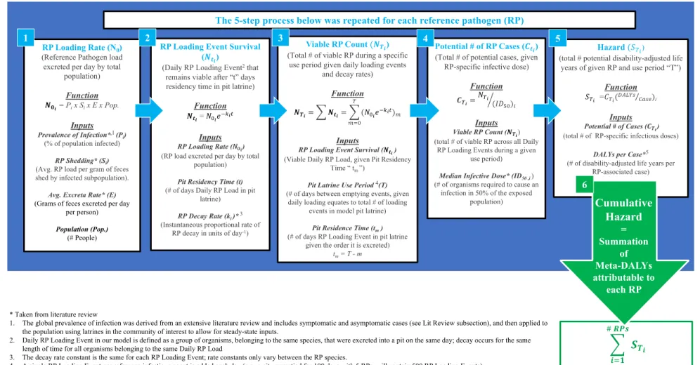
Our model is comprised of six components (summarized in Figure 1 and described in detail below). The first five components represent a five-step sequence that needs to be repeated for each reference pathogen species being modeled. The final component is the summation of the potential disease burdens attributable to each reference pathogen species. Microsoft Office Excel © software was used to manage the model data and perform the hazard analysis described in this paper.

2.1 List of Assumptions and Model Parameters

• Reference pathogens: A select number of pathogens are included in the model; each is referred to as a reference pathogen (RP). While our model is able to handle a large number of pathogen species, it is not likely a sanitation planner or engineer will have relevant information on all fecal-related disease causing agents, nor that they are all of major public health significance.

• Viable pathogens introduced daily: To simulate pit latrines in use, a fixed number of RPs are introduced daily4, 5_.

• Steady-state inputs: The daily loading rate for each reference pathogen is constant.

4_{Pathogen load= the daily load (number) of pathogens introduced each day in normal use.}

5_{Reference pathogen loading event is defined as a group of organisms, belonging to the same species, that were}

(17)

7

• Hazard was assessed on a community-scale: Each RP loading rate was quantified for total number of people using pit latrines in the community of interest, thus allowing us to average endemic infections, and assume a steady-state of inputs (e.g. constant daily loading rate) more reasonable6_.

• No leakage or overflow of pit latrine occurs: No pathogens lost through another route; pathogens only removed from pit latrine through pathogen die-off.

• Pathogen die-off is modeled by exponential first-order decay functions (N𝑡_𝑖= N_0𝑖e−k𝑖t) • No interaction between reference pathogens

• Determinants of Die-off7_{: Decay rate “}_k_i_{”, pit residency time or time passed since the RP loading}

event was excreted “t”, and the initial concentration of pathogens, which is equivalent to the

daily RP loading rate (𝑁0_𝑖).

• Decay rates “ki” constant across all cohorts comprised of same pathogen species: Decay rates

only vary between different pathogen species.

6_{For a single pit latrine, the users will recover from an infection relatively quickly and pathogen shedding will stop.}

(18)

Figure 1. Flow diagram of the pit latrine hazard model.

(19)

9

2.2 Reference Pathogen Loading Rate

[𝑁0]𝑖 = 𝑃𝑖 × 𝑆𝑖 × 𝐸 × 𝑃𝑜𝑝. Eq. 1

Equation 1 describes the first component of our model, and represents the reference pathogen loading rate for a given reference pathogen species. In Eq. 1, 𝑃𝑖 = the prevalence of infection in the population for a given reference pathogen, or the proportion of the population that is infected at a given time; 𝑆_𝑖= the reference pathogen shedding rate, or the number of organisms shed per gram of feces by an infected individual per day; E = the average fecal excretion rate, or the average grams of feces excreted per person per day; Pop. = the total number of people using pit latrines in the community of interest; i = specifies that this component was calculated individually for each reference pathogen. The loading rate is a per day rate; the group of organisms for a given reference pathogen excreted per day is hereafter referred to as a loading event. The reference pathogen loading rate describes inflow of

pathogens into the pit for our model, it is assumed constant over time, and is the model’s primary input.

The loading rate is determined for a community, rather than for a single household, to take advantage of the law of large numbers [Renze et al., 2017]. At this scale, assuming a constant daily loading rate, or steady-state inputs, is more reasonable. For example, for a single pit latrine, the users will recover from an infection relatively quickly and pathogen shedding will stop. However, if we consider an entire community, once one individual recovers from an infection another individual may develop the same infection and the pathogen loading rate remains constant over time. Finally, analyzing hazard at a community-scale, will likely be more helpful for public health officials and engineers as sanitation planning typically occurs at the district level and interventions involve multiple households.

2.3 Reference Pathogen Loading Event Survival "𝑵

𝒕𝒊"

[𝑵𝒕]𝒊 = 𝑁0𝑖𝑒−𝑘𝑖𝑡 Eq. 2

(20)

10

loading event was excreted into the pit “t”. A loading event is defined as a group of reference pathogens, belonging to the same species, excreted into the model pit latrine on the same day. In Eq. 2, 𝑁0_𝑖= the RP loading rate, or the total number of viable organisms excreted into the model pit latrine per day by total population, it is the primary outcome variable from component 1; e = is the mathematical constant that is the base of the natural logarithm [Marsden, 1985]; ki = the RP-specific decay rate8 reported in days-1,

which is assumed constant over time and for all RP loading events; t = pit residency time, or the number of days since the loading event was excreted into the model pit; i = specifies that this component was calculated individually for each reference pathogen.

Our reference pathogen loading event survival analysis used the first order exponential decay equation to describe inactivation kinetics [Rogers et al., 2011]. While it may oversimplify the death kinetics, the first order exponential decay equation is widely used in microbiology [Petrucci, 2007]. The only determinants of die-off (or survival) is ki the RP-specific decay rates, the initial concentration of RP

(equivalent to 𝑁0_𝑖the RP loading rate), and t the pit residence time. The authors are fully aware that environmental conditions (e.g. temperature, pH, moisture content, etc.) affect the rate of pathogen die-off. In our model the variation in these abiotic factors is captured in the decay rates ki.

A new loading event for a given reference pathogen species is added each day. Our model is based on the principle theory that pathogen decay begins upon the moment of excretion from a human host [Feachem et al., 1983]; a loading event excreted 200 days ago is likely to have far fewer viable pathogens present compared to a loading event excreted 1 day ago. To account for the temporal nature of pathogen excretions in pit latrines and the resulting effect on pathogen survival, we analyzed the survival of each loading event individually.

We assumed no leakage or overflow occurs between emptying events. In our model pathogens are only removed from the model pit between loading events by death or pathogen inactivation,

8_{Comprehensive literature reviews (section 4) were used to determine the RP-specific decay rates for the illustrative}

(21)

11

described by Eq. 2. Additionally, we assumed no interaction occurs between reference pathogens, so no predation or replication occurs in the model pit latrine.

2.4 Viable Reference Pathogen Count " 𝑵

𝑻𝒊"

[𝑵_𝑻]_𝒊 = [∑𝑇 (𝑁_𝑡)_𝑚

𝑚=0 ]𝑖 Eq. 3.1

𝑁_𝑇_𝑖= [∑𝑇 (𝑁_𝑡)_𝑚

𝑚=0 ]𝑖 = [∑𝑇𝑚=0(𝑁0𝑖𝑒−𝑘𝑖𝑡)_𝑚]_𝑖= 𝑁0𝑖(

1−𝑒−𝑘𝑖(𝑇+1)

1−𝑒−𝑘𝑖 ) Eq. 3.2

𝑡_𝑠 = 𝑇 − 𝑠 Eq. 3.3

Equation 3.1 describes the third component of our model, and represents the viable reference pathogen count [𝑁𝑇_𝑖], given a specified pit latrine use period “T” (number of days between pit emptying events). The total viable pathogen count is the summation of surviving pathogens across each loading

event (Eq. 3.1); “m” is the identifying index number for a given loading event.

When the summation of Eq. 3.1 is expanded out, it simplifies to Eq. 3.2 (see Annex for full derivation). In Eq. 3.2, 𝑁𝑡_𝑖= the number of surviving viable pathogens from a single daily loading event; 𝑁0_𝑖= the RP loading rate, or the total number of viable organisms excreted into the model pit latrine per day by total population; e = is the mathematical constant that is the base of the natural logarithm [Marsden, 1985]; ki = the RP-specific decay rate; t = pit residency time, or the number of days since

loading event was excreted into the model pit; T = pit latrine use period, or the time between emptying events, given daily loading events it is also equivalent to the total number of loading events in the model pit latrine for a given RP; i = specifies that the third component was calculated individually for each reference pathogen.

Given that we analyzed the survival of each loading event separately (Eq. 2) and the

(22)

12

residence time that was dependent upon the order in which the loading event was excreted into the model pit latrine (Eq. 3.3). In Eq. 3.3, tm = the pit residency time for a given loading event; m = is the

identifying index number for each loading event and correlates with the order in which the loading event was introduced into the model pit latrine (e.g. m = 0 is the first loading event excreted into the pit latrine and m = 1 was excreted a day later and is the second loading event added); T = the pit latrine use period.

It should be noted that while T = the pit latrine use period, or number of days between pit emptying events, it can also be thought as a measure of the pit emptying frequency. And given daily loading events it is also equivalent to the total number of loading events in the model pit latrine for each reference pathogen species. For example, if T = 100, then the pit is emptied every 100 days.

Additionally, if T = 100 and there are 3 reference pathogen species being modeled, there are a total of 300 loading events (100 for each reference pathogens species).

Components 1 – 3 characterize the pathogen behavior in the model pit latrine. The inflow, or pathogen flow rate, is described by component 1, and the subsequent outflow through pathogen die-off or inactivation is described by component 2. Component 3 describes the resulting total viable pathogen count for a given pit latrine use period. Components 4 – 6 are simply translations of component 3, the viable reference pathogen count.

2.5 Potential Number of Reference Pathogen Cases

“𝑪_𝒕_𝒊”

𝑪_𝑻𝒊 = [∑ 𝑁𝑇]𝑖

[𝐼𝐷50]𝑖 Eq. 4

Equation 4 describes the fourth component of our model, and represents the total number of potential cases, or infectious doses, present in the pit latrine sludge given a specified pit latrine use

period “T”. Potential cases are derived individually for each pathogen species being modeled (reference

pathogen). In Eq. 4, Ci = number of potential cases, the primary outcome variable for component 4;

(23)

13

variable derived in component 3; [𝐼𝐷50]𝑖 = the median infective dose for a given RP; i = specifies that this component was calculated individually for each reference pathogen. The total potential number of RP cases is simply a weighting of the viable RP count by infectivity (e.g. a translation of the viable count).

Our estimation of potential cases does not provide an estimate for actual cases that will occur as a result of the pathogens present in the pit latrine sludge. The number of pathogens required to cause an infection will not be doled out in perfect doses to a unique susceptible individual. Some people will ingest more organisms than is needed to cause an infection, others will not ingest enough, and others who ingest the organisms have already developed an immunity. Our results are meant to estimate the total potential cases to provide a measure of hazard, or potential public health threat.

2.6 Reference Pathogen Hazard

"𝑺

_𝑻_𝒊

"

𝑆𝑇𝑖 = C𝑇𝑖× ( 𝐷𝐴𝐿𝑌𝑠 𝐶𝑎𝑠𝑒⁄ )𝑖 Eq. 5

Equation 5 describes the fifth component of our model, and represents the total potential DALYs9 (Meta-DALYs) attributed to a given reference pathogen present in the pit sludge, given a specified pit

latrine use period “T”. In Eq. 5 (ST)i = the Meta-DALYs attributable to each RP for a given use period, the

primary outcome variable for component 5; 𝐶𝑇_𝑖 = the total potential RP cases, the primary outcome variable from component 4; _{( 𝐷𝐴𝐿𝑌𝑠 𝐶𝑎𝑠𝑒}⁄ )𝑖 = is the DALYs per prevalent case unique to each RP. DALYs per prevalent case was based off the 2015 global DALY estimates [GBD 2015] and the global prevalent cases [GBD 2015; Fletcher et al., 2011; Walker et al., 2010; Abba et al., 2009; Huilan et al., 1991] attributable to a given RP. DALYs are a measure of disease burden and therefore reflect disease severity. The RP Meta-DALYs is simply a translation of total potential cases to account for disease severity, and thus is a weighting of the viable RP count (component 3) by infectivity and disease severity.

(24)

14

We introduce Meta-DALYs, a new metric in our hazard assessment model. It is a measure of potential disease burden rather than the widely used measure of observed disease burden, DALYs (GBD 2015). The Meta-DALY is the primary measure of hazard in our model.

Components 1 - 5 represent a five-step sequence which is repeated for each reference pathogen species being modeled.

2.7 Cumulative Hazard

𝐶𝑢𝑚𝑢𝑙𝑎𝑡𝑖𝑣𝑒 𝐻𝑎𝑧𝑎𝑟𝑑_𝑇 = ∑5 𝑆_𝑇𝑖

𝑖=1 Eq. 6

The final component of our model is the summation of Meta-DALYs attributable to each reference pathogen 𝑆𝑇_𝑖, and is described by Eq. 6. The summation of RP Meta-DALYs estimates the cumulative hazard present in the population’s pit sludge, given a specified pit latrine use period “T”. It is the primary

outcome variable for our pit latrine hazard model introduced in this paper.

Our model is the first to explicitly represent pathogen hazards and their relative accumulation and decay in pit latrines over time. While admittedly conceptual, our pit latrine hazard model can provide practical insights. By providing a full look at the “natural history” of a given waste stream, it allows

(25)

15

CHAPTER 3: DESCRIPTION OF SIMULATED CASE STUDY

3.1 Description of Simulated Pit Latrine Case Study Parameters

To provide an illustrative example of the model, we applied it to a simulated case study of a 5,000 person population infected with five reference pathogens. The authors chose a common fecal indicator organism and the organisms attributed with the greatest global disability-adjusted life years (DALYs) from each of the four pathogen classes [GBD 2015] - E. coli spp., Rotavirus, Shigella spp., Cryptosporidium spp., and Ascaris. Reference pathogen-specific decay rates in the absence of treatment and the other required model inputs were determined through comprehensive literature reviews. The methods and results of the literature reviews are described in the following section (see Section 4).

3.2 Description of Comparative Analysis of Different Waste Streams

To gain a preliminary understanding of the public health significance of pit latrines relative to other sanitation waste we included three other identical10_{populations (total of four populations), each} using a different form of sanitation – 1) pit latrines; 2) open defecation; 3) sewerage with wastewater treatment that consistently removes 1-Log10 of all reference pathogens daily; and 4) sewerage with wastewater treatment that consistently remove 2-Log10 of all reference pathogens daily11. We estimate and compare the cumulative hazard attributable to each population’s waste streams.

10_{“identical” population refers to a 5,000 person population infected with the same five reference pathogens. As a}

result, the reference pathogen-specific loading rates and DALYs/prevalent case is the same for each population in our case study.

11_{These removal efficiencies cover the range of secondary wastewater treatments, except high quality membranes}

(26)

16

Open defecation (OD) refers to the practice whereby people defecate in open spaces (e.g. fields, open water bodies, etc.) rather than using a toilet [UNICEF and WHO, 2013]. With open defecation, pathogen hazards are immediately released into the environment; no die-off occurs in containment prior to release. For the purposes of this analysis, we equated OD with daily emptying in our model. Due to the differences in times scales of hazard discharge between pit latrines and OD (e.g. annual vs. daily), we converted cumulative hazard to average daily hazard discharged for pit latrines, given an average use period (e.g. number of days between pit emptying events) [Eq. 7].

(𝐴𝑣𝑔. 𝐷𝑎𝑖𝑙𝑦 𝐻𝑎𝑧𝑎𝑟𝑑 𝐷𝑖𝑠𝑐ℎ𝑎𝑟𝑔𝑒𝑑)_𝑇 = 𝐶𝑢𝑚𝑢𝑙𝑎𝑡𝑖𝑣𝑒 𝐻𝑎𝑧𝑎𝑟𝑑𝑇

𝑇 Eq. 7

With growing public health concerns and advances in technology, recent studies have examined pathogen removal efficiencies during different types of wastewater treatment. Primary treatment reportedly removes 0 – 1Log10 and most secondary treatment12 remove 0 – 2Log10 of the pathogen species investigated [WHO, 2006; Jimenez et al., 2010]. For the purposes of our analysis, we equated WW-treatment with 1-Log and 2-Log removal13_{efficiencies [Eq. 8; Eq. 9]. Similar to OD, there is a} difference in time scales between WW-treatment and pit latrines, therefore we also used average daily hazard discharged for pit latrines, given an average use period [Eq. 8] to allow for comparison of these two hazard estimations.

𝑂𝐷 𝑆

101 = 𝑊𝑊 1𝐿𝑜𝑔10 Eq. 8

𝑂𝐷 𝑆

102 = 𝑊𝑊 2𝐿𝑜𝑔10 Eq. 9

3.3 Sensitivity Analysis

The only determinants of pathogen survival in our model are the initial concentration of

pathogens (the magnitude is equivalent to the daily loading rate 𝑁0_𝑖 ), the pit residency time “t”, and the

12_{These removal efficiencies cover the range of secondary wastewater treatment technologies, except high quality}

membranes and chemical disinfection. Additionally, these removal efficiencies do not necessarily cover primary treatment paired with chemical disinfection [Jimenez et al., 2010; Ottson et al., 2006; Williams et al., 2015].

13_{For our analysis, we assumed consistent daily 1Log}₁₀_{and 2Log}₁₀_{removal of all pathogens for our sewerage and}

(27)

17

decay rate “ki “. The effect of variation in environmental conditions (e.g. temperature, pH, and moisture

(28)

18

CHAPTER 4: SUMMARY OF LITERATURE REVIEWS

4.1 Pathogen Decay Rates

–

Systematic Literature Review

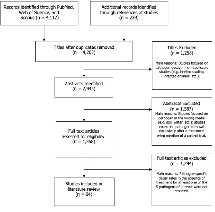
A systematic literature review was conducted to determine the rate of pathogen decay in excreta in the absence of treatment for the five reference pathogens (Rotavirus, Shigella spp., Cryptosporidium spp., Ascaris, and E. coli spp.) included in our model. We searched PubMed, SCOPUS, and Web of Science databases for studies that reported decay rates for at least one of the five reference pathogens in human excreta, feces, sludge, or animal manure. We included studies from peer-reviewed journals, textbooks, and grey literature published in English from any year. Many studies reported both treatment and non-treatment (control) trials; data from any non-treatment trials were included in the review and all data corresponding to treatment was excluded. Studies that examined decay in soil, on plants, in water, urine14_{, or from a clarified form of the pathogen were excluded (see full list of exclusion and inclusion} criteria in Table 1 below; see Figure 2 for literature review flow diagram below).

14_{The authors are aware excreta is defined as a mixture of feces and urine. Studies that examined clarified urine or}

(29)

19

(30)

20

Table 1. Inclusion and exclusion criteria for systematic literature review

Inclusion Criteria Exclusion Criteria

• Study examined at least one of the five reference pathogens

• Decay of pathogens recorded in human excreta, feces, sludge, and/or animal manure

• Static pile composting included

• Urine diverted pit latrine studies included

• Control trials in treatment studies included

• Studies that examine the effect of storage

• All years

• Types of Literature: Peer-reviewed journals, textbooks, grey literature, graduate student theses

• All trials that met the inclusion and exclusion criteria from the same study

• Chemical treatments

• Pit additives excluded except in the case of urine

• Aerated and turned composting excluded

• Waste stabilization pond studies excluded

• Wastewater treatment studies excluded

• Anaerobic and aerobic sludge digestion

• Any trials that just examined decay in urine

• Studies that did not report decay rates and/or exact time with an attributed quantity of removal

• Studies report decay rates in water, soil, seawater, or any other media that is not included in our inclusion criteria

We identified 4,356 papers for title and abstract screening. Sixty-four studies met our inclusion and exclusion criteria and were included in the final analysis. From the included studies, we extracted rate constants and the variables of each trial (e.g. temperature, pH, moisture content, pathogen detection method, and the excreta media) where available. The median rate constants were used in the main analysis presented in this paper. For the sensitivity analysis, interquartile range of decay rates for each reference pathogen was used. We present a summary of decay rates in Table 2 below for use in our simulated case study.

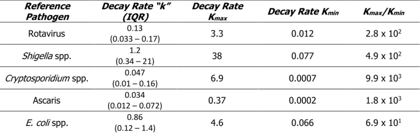
Table 2. Summary of Reference Pathogen Decay Rates “K” in fecal material in the absence of treatment.1

(All k values provided below are reported in days-1) Reference

Pathogen Decay Rate “k”(IQR) Decay Rate Kmax Decay Rate Kmin Kmax/Kmin

Rotavirus _(0.0330.13 _–_0.17) 3.3 0.012 2.8 x 102

Shigella spp. _(0.341.2 _–₂₁₎ 38 0.077 4.9 x 102

Cryptosporidium spp. _(0.010.047 _–_0.16) 6.9 0.0007 9.9 x 103

Ascaris _(0.0120.034 _–_0.072) 0.37 0.0002 1.8 x 103

E. coli spp. _(0.120.86 _–_1.4) 4.6 0.066 6.9 x 101

(31)

21

2013; Fischer et al., 2002; Fremaux et al., 2008; Fujioka et al., 2002; Ghigiletti et al., 1995; Ghigilletti et al., 1997; Gibbs et al., 1995; Gibson et al., 2014; Guan et al., 2003; Inoue et al., 2006; Jenkins et al., 1998; Jensen et al., 2008; Jensen et al., 2009; Jimenez et al., 2007; Katakam et al., 2013; King et al., 2007; Kuczynska et al., 1999; Lemos et al., 2005; Lepeuple et al., 2004; Magri et al., 2015; Magri et al., 2013; Martens et al., 2009; McKinley et al., 2012; Mehl et al., 2008; Mehl et al., 2011; Moe et al., 1982; Nakamura et al., 1965; Nasser et al., 2016; Nordin et al., 2009; Ogunyoku et al., 2016; Orstavik et al., 1974; Pandey et al., 2015; Paula et al., 2000; Paulsrud et al., 2004; Pecson et al., 2007; Pell et al., 1997; Peng et al., 2008; Pesaro et al., 1995; Polprasert et al., 1981; Pompeo et al., 2016; Robertson et al., 1992; Romero et al., 2014; Rose et al., 1997; Rze et al., 2004; Schmitz et al., 2016; Schonning et al., 2005; Stenstrom et al., 2002; Strauch, 1991; Trimmer et al., 2016; Turner et al., 1997; Vinneras, 2013; Wang et al., 1966; Williams et al., 2015; Ziemer et al., 2010

4.2 Pathogen Hazard Inputs

–

Review of Major Studies & Literature Reviews

Four literature reviews were conducted to determine the following inputs for each of our five

references pathogens (Rotavirus, Shigella spp., Cryptosporidium spp., Ascaris, and E. coli spp.), included in our pit latrine hazard model:

• Global disability-adjusted life years (DALYs) attributed to each reference pathogen; • Global prevalence of infection, including symptomatic and asymptomatic cases for all ages; • Median infective dose; and

• Pathogen shedding rate for infected individuals

Targeted Boolean searches were conducted in PubMed, Scopus, and Web of Science databases. Included literature for our review was limited to other literature reviews and major studies published in English. For studies concerning median infective dose and shedding rate all publication years were included. However, for studies concerning DALYs and prevalence of infection, papers published before 2010 were excluded in our review. Median figures for each of the five reference pathogens were determined from our literature review and included in our hazard model.

(32)

22

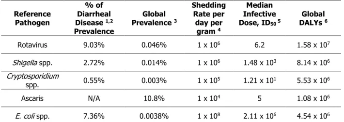
We present a summary of the average values for each input in Table 3 below for use in our simulated case study.

Table 3. Average value of each input

Reference Pathogen

% of Diarrheal Disease 1,2

Prevalence

Global Prevalence 3

Shedding Rate per

day per gram 4

Median Infective Dose, ID50 5

Global DALYs 6

Rotavirus 9.03% 0.046% 1 x 106 _6.2 _{1.58 x 10}7

Shigella spp. 2.72% 0.014% 1 x 106 _{1.48 x 10}3 _{8.14 x 10}6

Cryptosporidium

spp. 0.55% 0.003% 1 x 105 1.21 x 101 5.53 x 106

Ascaris N/A 10.8% 1 x 104 ₅ _{1.08 x 10}6

E. coli spp. 7.36% 0.0038% 1 x 108 _{2.11 x 10}6 _{4.54 x 10}6

1 Prevalence of diarrheal-related pathogens were reported as a percentage of global diarrheal disease prevalence in studies. Prevalence of Ascaris was not reported as a part of diarrheal-disease prevalence.

2. Fletcher et al., 2015; Platts-Mills et al., 2015; Fischer-Walker et al., 2010; Kotloff et al., 2013; Abba et al., 2010 3. GBD 2015; Brooker et al., 2010; Pullan et al., 2014

4. Feachem et al., 1983; Czumbel et al., 2016; Juilan et al., 2016; Fewtrell et al., 2015; WHO, 2005

5. Juilan et al., 2016; WHO, 2016; Feachem et al., 1983; DuPont et al., 1971; DuPont et al., 1972; Messner et al., 2001; Ward et al., 1986; Chapell et al., 2006; Strachan et al., 2005; Teunis et al., 2004; Haas et al., 2000; Powell et al., 2000; Niyogi, 2005; Levine et al., 1973; Crocket et al., 1996; Kotloff et al., 1995;

(33)

23

CHAPTER 5: LIMITATIONS

The major limitations of our pit latrine hazard model arise from five main sources:

1. Not considering exposure (quantifying hazard vs. risk);

2. Simplicity of the model inputs do not account for infectious disease dynamics;

3. Use of first-order exponential decay models to describe pathogen die-off (and survival); 4. Quality of data used in the simulated case study;

5. Method for defining the hazard attributed to other sanitation waste streams.

(1) Not Considering Exposure – Hazard vs. Risk. As a result of modeling hazard and not risk, exposure is not considered [WHO, 2016]. For microbial hazards, exposure is characterized by estimating the amount and the period of exposure to the pathogens [WHO, 2003]. Therefore, our model cannot provide an estimate of how likely the discharged excreta from different sanitation technologies will harm a

population. Our model estimates what is being discharged to the environment at the technological source (i.e. pit latrine), but does not account for varying levels of exposure after the excreta is discharged. In particular, our model does not account for the point of discharge into the environment. For example, if sewerage discharges to the ocean and pit latrines are emptied directly into the streets, the latter exposes a much larger population to infectious pathogens [WHO, 2016].

Exposure is an important variable to consider when trying to define what is “safe” and “unsafe”

[WHO, 2016; SFD Promotion Initiative, 2015]. However, the exposure routes for fecal pollution are numerous making risk assessments difficult to conduct [WHO, 2016]. Our method is simplistic and as a result easier to quantify. Estimating hazard at the origin, provides a basis for comparison of different

sanitation waste streams and provides the foundation for estimating the hazard attributed to “leaks”

along the sanitation service chain. However, since exposure and risk are not accounted for, caution

(34)

24

(2) Simplicity of Model and its Inputs. Our choice of constant pathogen loading rates, constant decay rates, and not explicitly accounting for the influence of environmental conditions on pathogen

decay imposes several restrictions on the model’s ability to represent infectious disease dynamics and as

a result the system accurately [Heesterbeck et al., 2015]. While, our model estimates hazard for the pit latrine waste stream of a community rather than an individual household allowing for some averaging, in the field there will be temporal fluctuations in the loading rate due to a number of factors that impact disease dynamics (e.g. developing immunities, seasonality of infections, outbreaks, etc.) [Heesterbeck et al., 2015]. By using constant decay rates and not explicitly accounting for environmental conditions, the seasonal trends in decay rates are also not captured. However, the simplicity of model inputs allows for a

more detailed temporal representation of a community’s pit latrine waste stream than would be possible

with other available methods.

(3) First-Order Exponential Decay Models. First-order exponential decay models may not be the best representation of die-off for all fecal-related pathogen species. From the limited microbiological studies, which have modeled pathogen decay in fecal material in the absence of treatment, it was found that certain organisms do not necessarily adhere to this decay structure [Berendes et al., 2015]. This may be particularly true for helminths [Berendes et al., 2015]. While first-order exponential decay models may oversimplify the death kinetics of some pathogen species, they are widely used in microbiology [Rogers et al., 2011]; the majority of decay rates found in the literature were determined for first-order exponential decay models [Rogers et al., 2011]. With advances in microbiological data, the incorporation of more sophisticated decay functions is possible in future iterations of our pit latrine hazard model.

(35)

25

well documented [Berendes et al., 2015; Schonning et al., 2005]. Additionally, there is only one source that reports the global disability-adjusted life years [GBD 2015].

Moreover, by the nature of literature reviews this collection of data, arises from various studies conducted at different times, under varying experimental conditions, for different purposes and was not necessarily developed to be integrated as we have done in our model. In particular, we derived an estimate for DALYs per prevalent case. While, DALYs reported by the GBD 2015 are based on reported prevalence, this figure was not available for any of the diarrheal disease pathogens [GBD 2015]. We determined a global prevalence from recent literature reviews and meta-analyses conducted [Fletcher et al., 2015; Platts-Mills et al., 2015; Fischer-Walker et al., 2010; Kotloff et al., 2013; Abba et al., 2010; GBD 2015; Brooker et al., 2010; Pullan et al., 2014] and applied this to the reported DALYs to determine the DALYs per prevalent case we used in our model.

(5) Defining Hazard for Other Waste Streams. No clear guidance exists on how to compare the relative hazards between the different sanitation waste streams. Very little literature exists concerning the relative pathogen content and hazard posed by open defecation or how it changes over time. The

guidelines associated with wastewater treatment are meant to control environmental pollution (e.g. biochemical oxygen demand, nitrogen, etc.) therefore the pathogen removal efficiency is highly variable and is just recently being extensively studied [WHO, 2006; Jimenez et al., 2010]. Additionally, the proportion of liquid (i.e. urine) and solid (i.e. feces) waste varies extensively between these different waste streams. The relative proportion of pathogens found in the solid versus liquid stream is also not well understood [Schonning et al., 2005; Hoglund et al., 2002]. The method we propose is relatively conceptual and the comparison is imperfect, but we believe it can still yield practical insights on relative hazards between the different sanitation technologies.

Problems with inputs and data will always exist for a conceptual model. The approach taken to model hazard in pit latrines is a technologically simple once, but we believe it will aid planners in better understanding the flow of pathogens through a pit latrine waste stream and allow for helpful

(36)

26

CHAPTER 6: RESULTS & DISCUSSION OF ILLUSTRATIVE CASE

STUDY

To the author’s knowledge, our model is the first to explicitly represent pathogen hazards and their relative accumulation and decay in pit latrines over time. A variety of informative results are available from our model. Direct and indirect outputs include: estimates of viable pathogen count, estimates of number of potential cases, estimates of cumulative pit latrine hazard measured in Meta-DALYs, estimates of hazard attributed to each reference pathogen, proportion of hazard contributed by recent loading events, and proportion of hazard reduced based on different management practices (e.g. pit emptying frequency). These results yield practical insights into pit latrine behavior as a treatment technology, and can lead to conclusions about management decisions.

To illustrate the kinds of results the model can produce we apply it to a case study of a 5,000 person population infected with five reference pathogens (RP) - Rotavirus, Shigella spp., Cryptosporidium spp., Ascaris, and E. coli spp (see Table 4 below for a summary of case study characteristics). The main body of analysis is conducted with median pathogen decay rates; the analysis is repeated considering the interquartile range of pathogen decay rates to determine how sensitive our results are to difference in rates of pathogen inactivity. While the model inputs used (prevalence of infection, shedding rates, median infective dose, and DALYs per prevalent case) reflect global averages, determined through comprehensive literature reviews, the authors do not intend the absolute numbers we present here to describe the magnitude of hazard posed by pit latrine waste globally. Rather we find the illustrative case study assists with understanding the temporal trends and general behavior of pathogen hazards in pit latrines under daily use conditions.

(37)

27

balances the exponential die-off of those already in the pit. With the parameter values of the model we used, the majority of cumulative hazard is contributed in the most recent month. As a result of these discoveries we found manipulating pit emptying frequency (or pit fill fates) and utilizing double pit

technology could have large impacts on the relative hazard posed by a community’s pit latrine waste

stream. Additionally, our model provided evidence that pit latrines operated with good management

practices discharge markedly less pathogen “pollution” relative to open defecation, can outperform

sewerage with wastewater treatment achieving 1-Log10 daily pathogen removal, and can perform comparably to sewerage with wastewater treatment achieving 2-Log10 daily pathogen removal.

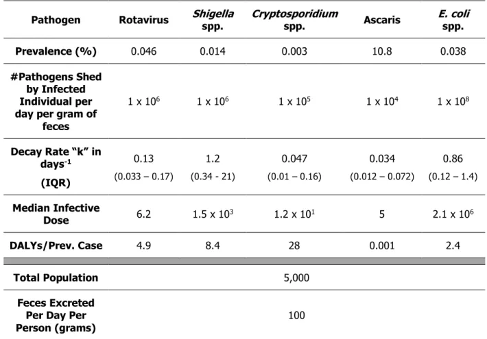
Table 4. Summary characteristics of illustrative case study.

Pathogen Rotavirus Shigella _spp. Cryptosporidium _spp. Ascaris E. coli _spp.

Prevalence (%) 0.046 0.014 0.003 10.8 0.038

#Pathogens Shed by Infected Individual per day per gram of

feces

1 x 106 _{1 x 10}6 _{1 x 10}5 _{1 x 10}4 _{1 x 10}8

Decay Rate “k” in days-1

(IQR)

0.13

(0.033 – 0.17)

1.2

(0.34 - 21)

0.047

(0.01 – 0.16)

0.034

(0.012 – 0.072)

0.86

(0.12 – 1.4)

Median Infective

Dose 6.2 1.5 x 103 1.2 x 101 5 2.1 x 106

DALYs/Prev. Case 4.9 8.4 28 0.001 2.4

Total Population 5,000

Feces Excreted Per Day Per Person (grams)

(38)

28

6.1 Characterizing Hazard Behavior and Management Implications

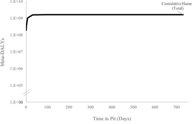
Figure 3. Cumulative hazard (DALYs) determined for the model pit latrine; summation of Meta-DALYs attributable to each reference pathogen.

Figure 3 presents the cumulative hazard (Meta-DALYs) determined. Cumulative hazard is summation of potential disease burden attributed to each of the five reference pathogens. We estimated cumulative hazard posed by the 5,000 person pit latrine waste stream on day 1 to be 1.86 x 108 Meta-DALYs and it increases to 1.54 x 109 _{Meta-DALYs by day 730.}

(39)

29

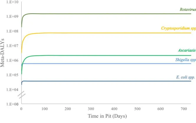
attributed to E. coli spp. increases from 2.10 x 104 _{Meta-DALYs (day 1) to 3.64 x 10}4 _{Meta-DALYs (day} 730).

Figure 4. Meta-DALYs attributable to each reference pathogen in model pit latrine over two-year period.

6.1.1 Checking model numbers

Comparing model output with figures reported in the literature is a first check on whether the model and its results may be reasonable. Since there has been no direct measurement of latrine hazard, we must work indirectly with other data.

(40)

30

al., 2007; Chien et al., 2002; Stenstrom et al., 2002]. The pathogen concentrations found in our model are within the range seen in the literature15_.

Our reported cumulative Meta-DALYs (1.54 x 109_{) for a population of 5000 are large; the} Meta-DALYs we report are greater than the annual global diarrheal disease Meta-DALYs (7.1 x 108 _{DALYs)! [GBD,} 2015; Fletcher et al., 2011; Walker et al., 2010; Abba et al., 2009; Huilan et al., 1991]. However, The DALYs reported in the GBD study were calculated from recorded infections [GBD, 2015], whereas our study reports potential DALYs, and do not reflect actual infections.

6.1.2 Why do we see an increase in hazard?

We observed an increase in the viable RP count for all five included RPs and as a result an increase in cumulative hazard, by approximately an order of magnitudewith no subsequent decrease (see Figure 4). The majority of microbiological studies in the WaSH field examine the behavior of a single pathogen cohort (e.g. a closed system) under varying experimental conditions. Our model studies a pit latrine system in use (e.g. an open system) and therefore includes a continuous daily inflow of viable pathogens (see Figure 1 for flow diagram of methods). Given that the RP loading rate for our model is constant, we can expect the cumulative hazard to increase with time.

15_{Our pathogen concentrations were calculated under the assumption of conservation of mass. The authors are}

(41)

Figure 5. Visual representation of how multi-loading event model structure used in this paper differs from the conventional single loading event study structure. Time (Days) V ia b le R P C o u n t (# o rg an is m s)

Decay of a Single RP Cohort (i.e. loading event)1

Time (Days) V ia b le R P C o u n t (# o rg a n is m s)

Decay of Multiple RP Loading Events Occurring in Parallel

Sum of Viable RP Count Across All2Daily Loading Events

V ia b le R P C o u n t (# o rg an is m s) Time (Days)

We sum the qty. of viable RP at each

time point.

A loading event is added each day. Our

model tracks the decay of each loading

event. Most studies examine the decay of a

single cohort (i.e. loading event)

When we examine the trend of viable RP over time of all daily loading events we see:

1) There is an increase in the beginning; and 2) A steady-state is eventually reached. The decay of each loading events occurs in

parallel. Our model sums the quantity of viable RP at each time point.

1_{Loading Event}_{is defined as a group of organisms belonging to a single RP species (e.g.}_{Rotavirus or E.coli}_{) that were excreted at the same time; decay starts and occurs for the same length of}

time for all organisms in a single loading event. The rate of decay does not vary between loading events of the same RP species.

2_{Sum of viable RP count was calculated across all daily loading events for a single RP species; the process was repeated for each of the 5 RP included in our illustrative case study.}

The viable RP count is then

weighted by infectivity and disease

severity and converted to

Meta-DALYs

(42)

32 6.1.3 Steady-state behavior

In addition to an increase in cumulative hazard with time, we observed cumulative hazard

reached a constant level and therefore obtained a steady state equilibrium (see Figure 3). To the author’s

knowledge, steady-state pathogen behavior has not been reported in other WaSH studies [Ogynyoku et al., 2016; Berendes et al., 2015; Jimenez et al., 2007; Chien et al., 2002; Stenstrom et al., 2002]. However, steady state behavior has been widely documented in microbial ecology, where open-systems are more commonly considered [Hsu et al., 1991; Dung et al., 1997; Hanemaajier et al., 2015]. This finding provides evidence that even under use conditions, the public health hazard from on-site sanitation does not increase indefinitely with time.

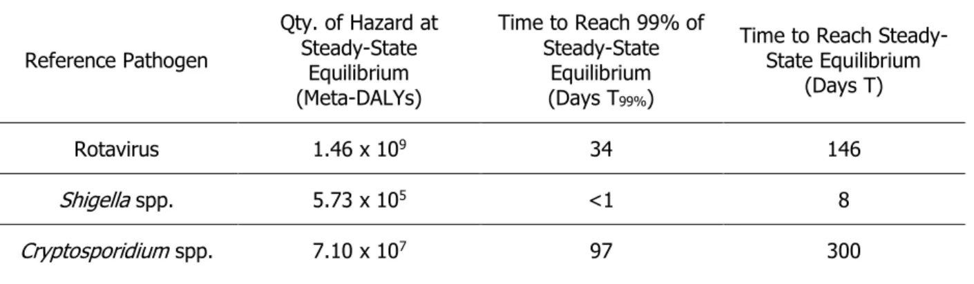
The time required to reach steady state16_{is dependent upon the RP-specific decay rate (Eq. 10).} Rapidly decaying microorganisms, such as Shigella spp. and E. coli spp. achieved a steady state within 20 days. In contrast, Ascaris required 271 days to achieve an absolute constant equilibrium (NOTE: By day 100, all five RP reached ≥99% of their absolute steady-state equilibrium level). Despite the varying persistence of RP species in our model, we find all organisms reach a steady state equilibrium within one year, under daily use conditions (see Table 5).

lim

𝑡→ ∞𝑁𝑡 = 𝑁0

(1−𝑒−𝑘₎ Eq. 10

Table 5. Description of hazard (Meta-DALYs) at steady-state equilibrium.

Reference Pathogen

Qty. of Hazard at Steady-State

Equilibrium (Meta-DALYs)

Time to Reach 99% of Steady-State

Equilibrium (Days T99%)

Time to Reach Steady-State Equilibrium

(Days T)

Rotavirus 1.46 x 109 ₃₄ ₁₄₆

Shigella spp. 5.73 x 105 _<1 ₈

Cryptosporidium spp. 7.10 x 107 ₉₇ ₃₀₀

16_{By Eq. 11 a steady-state, or constant value, will not be reached but it will be approached asymptomatically. When}

(43)

33

Ascaris 3.19 x 106 ₉₉ ₂₇₁

E. coli spp. 3.64 x 104 ₄ ₁₁

Cumulative (TOTAL) 1.54 x 109 ₉₉ ₃₅₃

Finding a steady state long-run level of hazard in latrines is a mathematical result of utilizing first-order log-linear decay models with constant inputs and constant decay rates (see Methods Section 2.2 –

2.3) [Wade et al., 2015; Hsu et al., 1983]. Altering this component of our model, could result in changes to our steady-state findings. For instance, if the dynamic nature of environmental factors such as

seasonal fluctuations in temperature or competition among pathogens for resources, was accounted for, variations in inputs and decay rates would arise [Mehl et al., 2011; Feachem et al., 1983]. In theory, steady state levels would exist but they would fluctuate with the fluctuations in inputs and decay rates.

Additionally, while first-order log-linear decay models are the most used to describe pathogen inactivation in the literature [see Sys. Lit Review Section 4.1], recent studies report that survival curves

for some pathogen species are often nonlinear and may exhibit a “recalcitrant” long tail [Bevilacqua et al., 2015; Marks et al., 2007]. Moving away from first-order inactivation kinetics towards non-linear decay models, has two major implications on our findings. As mentioned above, it is possible that our steady state equilibrium finding, even theoretical, may no longer be valid. Also, according to the literature, a long tail signifies the existence of a more resistant subpopulation [Marks et al., 2007; Li et al., 2007]. If we accept this theory, then our results found using first-order log-linear decay models are likely

(44)

34

6.1.4. Implications of steady-state behavior: pit emptying frequency

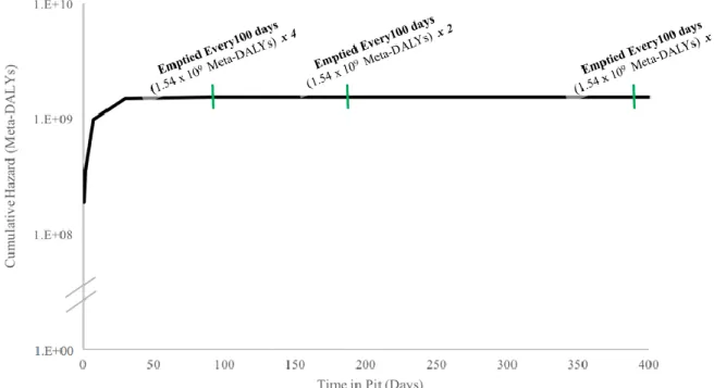
Our findings suggest that long periods between emptying (provided they do not lead to overflows!) are better from a public health perspective. If we consider each pit emptying event as a discharge of pathogens (e.g. hazard) into the environment, our model suggests the longer a pit remains unemptied the less total cumulative hazard is discharged into the environment over time, assuming no leakage or overflow. This may not immediately be intuitive from Figure 3. From the graph of cumulative hazard over time, we can determine the quantity of hazard that would be discharged upon pit emptying at any given point in time (see Figure 6). For example, if the pit latrine was emptied at 100 days the cumulative hazard discharged would be approximately 1.54 x 109_{Meta-DALYs, and if the pit latrine was} emptied at 200 days the cumulative hazard discharged would also be approximately 1.54 x 109 Meta-DALYs. However, these are point values; they do not provide a total cumulative hazard discharged to the environment over the same time frame. In Figure 6, we demonstrate that given approximately equivalent point values due to the steady-state nature of our model, a pit emptied every 100 days essentially

discharges 2x the total cumulative hazard to the environment compared to a pit emptied every 200 days.

(45)

35

Total cumulative hazard discharged to the environment is reduced by the pathogen die-off that occurs in a pit latrine prior to emptying. From our model, we can estimate the total cumulative hazard averted with different emptying frequencies (see Figure 7). For example, if we consider the extreme case of daily emptying as our base, a switch to emptying every two-years reduces total cumulative hazard discharged to the environment by approximately 99%. Adjusting pit emptying frequency takes advantage of the naturally occurring pathogen die-off in pit latrines, and can reduce the public health hazard posed by on-site sanitation.

Figure 7. Percentage change in cumulative hazard (Meta-DALYs) discharged into the environment with different pit latrine emptying frequencies (base = daily emptying).

Currently the primary focus of safe fecal sludge management (FSM) for on-site sanitation is examining hygienic pit latrine emptying services and excreta disposal [Foxon et al., 2011; Jenkins et al., 2015; Thye et al., 2012; Jenkins et al., 2012; Opel et al., 2013]. While these are two important FSM considerations, our model provides evidence that encouraging management practices that reduce pit emptying frequency can also have a strong public health impact. Emptying frequency is largely dictated by sludge accumulation rates [Jenkins et al., 2015; Zwia et al., 2016a; Zwia et al., 2016b; Still et al., 2012]. Zzwia et al. (2016a) found pit latrines in Kampala filled up faster than expected due to

-34% -74% -91% -95% -98% -99%

-100% -90% -80% -70% -60% -50% -40% -30% -20% -10% 0%

Weekly Monthly 3 Months 6 Months Annually 2 Yrs

Change in Cumulative Hazard (% Meta-DALYs)

(46)

36

“inappropriate” use, in particular using pits for disposal of solid waste. They report that public pit latrines actually had slower accumulation rates compared to private latrines partly due to the restriction of solid waste disposal. Jenkins et al. (2015) found pit latrines previously emptied required more frequent emptying into the future due to a failure of available pit emptying methods to remove all of the contents of full pits. While the rate of sludge accumulation is largely dictated by biological and environmental factors that are not easily influenced by pit latrine users [Foxon et al., 2011], there is evidence that certain behaviors such as proper solid waste disposal and complete pit emptying may have a positive public health impact by reducing pit emptying frequency.

6.1.5 Recent loading events are the most hazardous, but by how much?

The conventional belief that the most recent excreta loading events are the most hazardous [Feachem et al., 1983] is supported by our model. Given a two-year use period, we estimated

approximately 12.5% of total cumulative hazard is contributed by the most recent day’s load and nearly

97% is contributed by the most recent month’s load (see Figure 8).

Figure 8. Proportion of Meta-DALYs contributed from recent loading events (day, week, and month) given a two-year use period.

0% 10% 20% 30% 40% 50% 60% 70% 80% 90% 100%

Rotavirus Shigella Cryptosporidium Ascaris E.coli Total

Proportion of Meta-DALYs Contributed by Recent Loading Events (% Meta-DALYs)

Month