ISSN 1440-771X
Australia
Department of Econometrics and Business Statistics
http://www.buseco.monash.edu.au/depts/ebs/pubs/wpapers/
October 2010
Working Paper 18/10
A Bayesian approach to parameter estimation for kernel density
estimation via transformations
A Bayesian approach to parameter estimation for kernel density
estimation via transformations
Qing Liu∗,1, David Pitt2, Xibin Zhang3, Xueyuan Wu1
1Centre for Actuarial Studies, Faculty of Business and Economics, The University of Melbourne 2Department of Actuarial Studies, Faculty of Business and Economics, Macquarie University
3Department of Econometrics and Business Statistics, Monash University
September 2010
Abstract
In this paper, we present a Markov chain Monte Carlo (MCMC) simulation algorithm for estimating parameters in the kernel density estimation of bivariate insurance claim data via transformations. Our data set consists of two types of auto insurance claim costs and exhibit a high-level of skewness in the marginal empirical distributions. Therefore, the kernel density estimator based on original data does not perform well. However, the density of the original data can be estimated through estimating the density of the transformed data using kernels. It is well known that the performance of a kernel density estimator is mainly determined by the bandwidth, and only in a minor way by the kernel choice. In the current literature, there have been some developments in the area of estimating densities based on transformed data, but bandwidth selection depends on pre-determined transformation parameters. Moreover, in the bivariate situation, each dimension is considered separately and the correlation be-tween the two dimensions is largely ignored. We extend the Bayesian sampling algorithm proposed by Zhang, King and Hyndman (2006) and present a Metropolis-Hastings sampling procedure to sample the bandwidth and transformation parameters from their posterior den-sity. Our contribution is to estimate the bandwidths and transformation parameters within a Metropolis-Hastings sampling procedure. Moreover, we demonstrate that the correlation between the two dimensions is well captured through the bivariate density estimator based on transformed data.
Key words: bandwidth parameter; kernel density estimator; Markov chain Monte Carlo; Metropolis-Hastings algorithm; power transformation; transformation parameter.
JEL Classification: C14, C15, C63
∗Corresponding author. Centre for Actuarial Studies, Faculty of Business and Economics, The University of
1
Introduction
Kernel density estimation is one of the widely used non-parametric estimation techniques for estimating the probability density function of a random variable. For a univariate random variable X with unknown density f(x), if we draw a sample of nindependent and identically distributed observationsx1, x2, . . . , xn, the kernel density estimator is given by
ˆ f(x) = 1 n n X i=1 1 hK µ x−xi h ¶ ,
wherehis the bandwidth that controls the amount of smoothness, andK(·) is the kernel function which is usually chosen to be a symmetric density function. Wand, Marron and Ruppert (1991) argued that the classical kernel density estimator does not perform well when the underlying density is asymmetric because such an estimation requires different amounts of smoothing at different locations. Therefore, they proposed to transform the data with the intention that the use of a global bandwidth is appropriate for the kernel density estimator after transformation. The power transformation is one such transformation for this purpose.
There are a number of alternative transformation methods that have been studied in the literature. For example, Hjort and Gald (1995) advocated a semi-parametric estimator with a parametric start. Clements, Hurn and Lindsay (2003) introduced the Mobius-like transfor-mation. Buch-Larsen, Nielsen, Guillen and Bolance (2005) proposed an estimator obtained by transforming the data with a modification of the Champernowne cumulative density function and then estimating the density of the transformed data through the kernel density estimator. These transformation methods are particularly useful with insurance data because the distri-butions of insurance claim data are often skewed and present heavy-tailed features. However, these transformations often involve some parameters, which have to be determined before the kernel density estimation is conducted. In this paper, we aim to present a sampling algorithm to estimate the bandwidth and transformation parameters simultaneously.
It is well established in the literature that the performance of a kernel density estimator is largely determined by the choice of bandwidth and only in a minor way, by kernel choice (see for example, Izenman, 1991; Scott, 1992; Simonoff, 1996). Many data-driven bandwidth selection methods have been proposed and studied in the literature (see for example, Marron, 1988). However, Zhang, King and Hyndman (2006) pointed out that kernel density estimation for multivariate data has received significantly less attention than its univariate counterpart
due to the increased difficulty in deriving an optimal data-driven bandwidth as the dimension of the data increases. They proposed MCMC algorithms to estimate bandwidth parameters for multivariate kernel density estimation.
The data set we use in this paper has two dimensions, and therefore we could use Zhang, King and Hyndman’s (2006) MCMC algorithm to estimate bandwidth parameters. However, their algorithm has so far only been used to estimate a density for directly observed data. As our data are highly positively skewed and have to be transformed for the purpose of density estima-tion, we extend their MCMC algorithm so that it estimates not only the bandwidth parameters but also the transformation parameters for the bivariate insurance claim data. Bolance, Guillen and Nielsen (2008) analysed the same data using the kernel density estimation via transfor-mations, but they estimated the transformation parameters by dealing with each dimension separately. Their approach ignores any possible correlation between the variables of the data set. In this paper, we present MCMC algorithms for estimating the bandwidth and transfor-mation parameters for not only univariate data but also bivariate data. We investigate the differences in estimated correlations calculated through both sampling algorithms.
The rest of the paper is organised as follows. In Section 2, we provide a brief summary of the data and demonstrate the motivation for the paper. Section 3 presents MCMC algorithms for estimating bandwidth parameters and transformation parameters for kernel density estimation via transformations for univariate and bivariate data. In Section 4, we examine the performance of our MCMC algorithms in choosing bandwidths and estimating transformation parameters for the bivariate insurance claim data in comparison with other well known bandwidth selectors. Section 5 concludes the paper.
2
Data and motivation
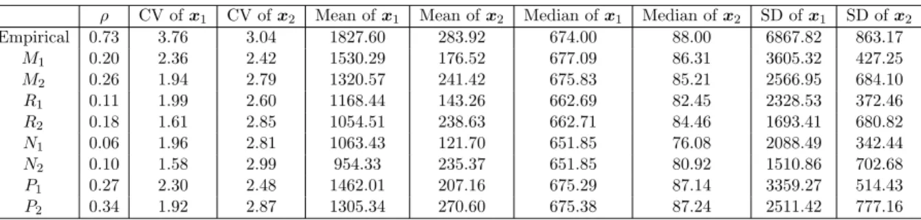
Our data set is the one analysed by Bolance, Guillen and Nielsen (2008). This set of data was collected from a major automobile insurance company in Spain. The data contain 518 paired claims. Each claim contains two types of losses, which are respectively, property damageX1 and
medical expense X2. It is intuitive that a serious car accident might cause serious damage to
the cars, and the passengers involved in the accident might also be seriously injured. Therefore, we expect that the two types of claims are positively correlated.
costs, as well as a scatter plot of the logarithms of such claim costs. The two graphs suggest that there exists a significant positive correlation between the two types of costs.
Bolance, Guillen and Nielsen (2008) investigated modelling these data using both the clas-sical kernel density estimation method and the transformed kernel density estimation method. They found that the transformed kernel estimation approach obviously performs better than the classical kernel estimation method in terms of conditional tail expectation (CTE) calculations. However, they chose both the bandwidth and transformation parameters by dealing with each variable separately. Their bandwidth and transformation parameter selection method ignores any possible correlation between X1 and X2. In this paper, we propose to estimate the
band-width and transformation parameters for the bivariate data through our new Bayesian sampling algorithm.
3
A Bayesian sampling algorithm
3.1 Kernel density estimationThe kernel density estimation technique is often of great interest in estimating the density for a set of data. However, when the underlying true density has heavy tails, the kernel density estimator (with a global bandwidth being used) can perform quite poorly. Wand, Marron and Ruppert (1991) suggested transforming the data and obtaining the kernel density estimator for the transformed data. The density estimator for the untransformed data is the derived kernel density estimator for the transformed data multiplied by the Jacobian of such a transforma-tion. Wand, Marron and Ruppert (1991) found that compared to working with kernel density estimation for untransformed data, significant gains can be achieved by working with density estimation for transformed data.
The shifted power transformation is one such transformation that is effective in changing the degree of skewness in positive data (see for example, Wand, Marron and Ruppert, 1991). Such a transformation is given by
˜
y= ˜Tλ1,λ2(x) = (
(x+λ1)λ2sign(λ2) ifλ26= 0
ln(x+λ1) ifλ2= 0 ,
preserving, ˜y is further transformed as y=Tλ1,λ2(x) = µ σx σy˜ ¶ ˜ y, whereσ2
xandσy2˜are the variances ofxand ˜y, respectively. Letyi =Tλ1,λ2(xi), fori= 1,2,· · ·, n.
The kernel density estimator for the univariate transformed data is ˜ fh,λ1,λ2(y) = 1 n n X i=1 1 hK µ y−yi h ¶ ,
and the kernel density estimator for the untransformed data is ˆ fh,λ1,λ2(x) = 1 n n X i=1 1 hK µ Tλ1,λ2(x)−Tλ1,λ2(xi) h ¶ Tλ01,λ2(x).
Wand, Marron and Ruppert (1991) investigated data-driven selection methods for the choice of transformation parameters and bandwidth or smoothing parameter for univariate data. How-ever, the transformation parameters have to be pre-determined for chosen bandwidths. More-over, when the dimension of data increases, the estimation of these parameters becomes increas-ingly difficult. In this paper, we aim to estimate the transformation parameters and bandwidth parameters simultaneously.
3.2 Bivariate kernel density estimation via transformation
Let xi = (xi1, xi2)>, for i= 1,2,· · ·, n, denote the original data, and let the transformed data
be denoted as yi = (yi1, yi2)> = (Tλ11,λ21(xi1), Tλ12,λ22(xi2))>, for i = 1,2,· · · , n. The kernel
density estimator for the bivariate transformed data is given by ˆ f(y1, y2) = n1 n X i=1 1 h1h2K µ y1−yi1 h1 , y2−yi2 h2 ¶ , (1)
whereh1andh2 are bandwidths for the two dimensions, andK(·,·) is a bivariate kernel function
which is usually the product of two univariate kernels. Therefore, this bivariate kernel estimator can be re-written as ˆ f(y1, y2) = 1 n n X i=1 1 h1 K µ y1−yi1 h1 ¶ 1 h2 K µ y2−yi2 h2 ¶ . (2)
The bivariate kernel density estimator for the original data is ˆ fh,λ1,λ2(x) = 1 n n X i=1 ( 2 Y k=1 1 hkK µ Tλ1k,λ2k(xk)−Tλ1k,λ2k(xik) hk ¶ Tλ01k,λ2k(xk) ) , (3)
where x= (x1, x2)>, h = (h1, h2)> is a vector of bandwidths, λ1 = (λ11, λ21)> is a vector of
transformation parameters forx1, andλ2 = (λ12, λ22)>is a vector of transformation parameters
forx2.
Two limitations of using kernel density estimation via transformations are given in the lit-erature. First, the transformation parameters have to be pre-determined so that bandwidth parameters can be chosen through some currently available method. Second, when estimat-ing the density of the insurance claim data, Bolance, Guillen and Nielsen (2008) obtained the marginal kernel density estimator via transformations. They derived the CTE through the es-timated marginal densities. As a consequence, their approach ignores any possible correlation between the two dimensions. In this paper, we present the posterior density of the bandwidth parameters and transformation parameters. A Metropolis-Hastings sampling procedure is pre-sented to sample both types of parameters from their posterior.
3.3 Bayesian sampling algorithms
Zhang, King and Hyndman (2006) presented a MCMC simulation algorithm for sampling band-width parameters from their posterior density based on directly observed data. When data are transformed through some transformation parameters, a kernel-form estimator of the density for the original data can be constructed through the kernel density estimator for the transformed data. Such a density estimator is given by (3), which is a function of bandwidth parameters and transformation parameters. We find that their sampling algorithm can be extended to sample bandwidth parameters and transformation parameters from their joint posterior constructed through (3).
3.3.1 Univariate kernel density estimation
We estimated the bandwidth and transformation parameters for the kernel density estimator via transformation for univariate dataxk, fork= 1 and 2. In this way, any possible correlation betweenx1 andx2 is ignored. For each dimension, we have three unknown parameters, namely
transfor-mation family). The posterior density of these three parameters can be obtained through the likelihood cross-validation criterion in the same way as what Zhang, King and Hyndman (2006) did. We assume that the prior density ofhk is the normal density with meanµhk and standard deviationσhk: p0(hk) = q 1 2πσ2 hk exp ( −(hk−µhk)2 2σ2 hk ) ,
fork = 1 and 2. The prior density of λ1k is the normal density with mean µλ1k and standard deviationσλ1k: p1(λ1k) = 1 q 2πσ2 λ1k exp ( −(λ1k−µλ1k)2 2σ2 λ1k ) ,
fork= 1 and 2. The prior density ofλ2k is the uniform density U(−ak,1),
p2(λ2k) = 1 +1a
k,
fork= 1 and 2. Therefore, the joint prior density of (hk, λ1k, λ2k) is
p(hk, λ1k, λ2k) =p0(hk)×p1(λ1k)×p2(λ2k),
fork= 1 and 2, where the hyperparameters are µhk,σhk,µλ1k,σλ1k and ak. The likelihood is approximated as `k(xk|hk, λ1k, λ2k) = n Y i=1 ˆ f(i),hk,λ1k,λ2k(xik),
where the leave-one-out estimator is given by ˆ f(i),hk,λ1k,λ2k(xik) = n−1 1 n X j=1;j6=i 1 hkK µ Tλ1k,λ2k(xik)−Tλ1k,λ2k(xjk) hk ¶ Tλ01k,λ2k(xik), fork= 1 and 2.
According to Bayes theorem, the posterior of (hk, λ1k, λ2k) is (up to a normalising constant)
π(hk, λ1k, λ2k|x1k, x2k,· · ·, xnk)∝p(hk, λ1k, λ2k)×`k(xk|hk, λ1k, λ2k), (4) for k= 1 and 2. We are able to simulate (h1, λ11, λ21) and (h2, λ12, λ22) from (4) with k= 1
and k = 2, respectively. The ergodic average or the posterior mean of each parameter acts as an estimate of that parameter. In terms of univariate kernel density estimation discussed here, our contribution is to present a sampling algorithm that aims to estimate both types
of parameters for univariate data. Hereafter, we call this sampling algorithm the univariate sampling algorithm.
3.3.2 Bivariate kernel density estimation
Given bivariate observations denoted asxi, fori= 1,2,· · · , n, and the parameter vector denoted
as (h,λ1,λ2), the likelihood function is approximated as (H¨ardle, 1991)
`(x1,x2,· · ·,xn|h,λ1,λ2) = n Y i=1 ˆ f(i),h,λ1,λ2(xi), (5) where ˆ f(i),h,λ1,λ2(xi) = n−1 1 n X j=1;j6=i ( 2 Y k=1 1 hkK µ Tλ1k,λ2k(xik)−Tλ1k,λ2k(xjk) hk ¶ Tλ01k,λ2k(xk) ) , (6)
which is the leave-one-out estimator of the density of xi, fori= 1,2,· · · , n.
Let the joint prior density of (h,λ1,λ2) be denoted asp(h,λ1,λ2), which is the product of
marginal priors defined in Section 3.3.2. Then the posterior of (h,λ1,λ2) is (up to a normalising
constant)
π(h,λ1,λ2|x1,x2,· · · ,xn)∝p(h,λ1,λ2)×`(x1,x2,· · · ,xn|h,λ1,λ2), (7) from which we can sample (h,λ1,λ2) through an appropriate sampling procedure, such as the
Metropolis-Hastings sampling procedure described as follows.
1) Conditional on (λ1,λ2), we sample hfrom (7) using the Metropolis-Hastings algorithm.
2) Conditional on h, we sample (λ1,λ2) from (7) using the Metropolis-Hastings algorithm. The sampling algorithm in the first step is the same as the one presented by Zhang, King and Hyndman (2006) for directly observed data. Alternatively, we can sample (h,λ1,λ2) directly
from its posterior density given by (7) using the Metropolis-Hastings algorithm. Hereafter, we call this sampling algorithm the bivariate sampling algorithm.
3.4 An application to bivariate insurance claim data
In order to explore the benefits that could be gained by estimating the parameters using bivariate data instead of separately estimating density for each dimension of data, we apply the MCMC algorithms proposed in Section 3.3 in two ways and compare the two sets of results.
First, we estimated (hk, λ1k, λ2k) for the kernel density estimator of each variable based on
univariate data xk, for k= 1 and 2, using the sampling algorithm presented in Section 3.3.1.
The hyperparameters were chosen to beµhk = 40 andσhk = 5, fork= 1 and 2, andµλ11 = 1500, σλ11 = 333, µλ12 = 90,σλ12 = 30 and ak= 6, for k= 1 and 2.
Second, we estimated the bandwidth vector h, the transformation parameter vectors λ1
and λ2 for the bivariate density estimator for the bivariate data using the sampling algorithm
presented in Section 3.3.2. The hyperparameters were chosen to beµhk = 40,σhk = 5 fork= 1 and 2,µλ11 = 2300,σλ11 = 1000,µλ12 = 40, σλ12 = 20,a1 = 5 anda2 = 2.
We are particularly interested in the correlation coefficient captured through both sampling algorithms. We wish to know whether the correlation between the two dimensions can be better captured using the bivariate sampling algorithm than with the univariate sampling algorithm. We calculate the Pearson’s correlation coefficient betweenX1 and X2 using the estimated
den-sities with the formula
ρ=Corr(X1, X2) = q£ E(X1X2)−E(X1)E(X2) E(X2 1)−E2(X1) ¤ £ E(X2 2)−E2(X2) ¤ , (8) where E(Xi) = R∞ 0 xif(xi)dxi, E(Xi2) = R∞
0 x2if(xi)dxi, for i = 1 and 2, and E(X1X2) =
R∞
0
R∞
0 x1x2f(x1, x2)dx1dx2. Using the rectangle method, we wrote R functions to numerically
approximate the integrals and the double integral in the above expression. Our programs allow for controlling the accuracy of the integrals. We tested our numerical computation on bivariate normal distributions with known densities and found the error to be less than 0.01%.
4
Results and discussion
4.1 MCMC resultsAs previously discussed in Section 3.2, we executed both the the univariate and bivariate sam-pling algorithms. Table 1 presents the results obtained by running the univariate samsam-pling algorithm for each of the two variables separately, ignoring any possible correlation between the two variables. Table 2 provides the results derived by running the bivariate sampling algorithm for the bivariate data.
To prevent false impressions of convergence, we chose the tuning parameter in the random-walk Metropolis-Hastings algorithm so that the acceptance rate was between 0.2 and 0.3 (see for
example, Tse, Zhang and Yu, 2004). The burn-in period was chosen to contain 5,000 iterations, and the number of total recorded iterations was 10,000. The simulation inefficiency factor (SIF) was used to check the mixing performance of the sampling algorithm (see for example, Roberts, 1996). The SIF can be approximated as the number of consecutive draws needed so as to derive independent draws. For example, if the SIF value is 20, we should retain one draw for every 20 draws so that the retained draws are independent(see for example, Kim, Shephard and Chib, 1998; Meyer and Yu, 2000; Zhang, Brooks and King, 2009).
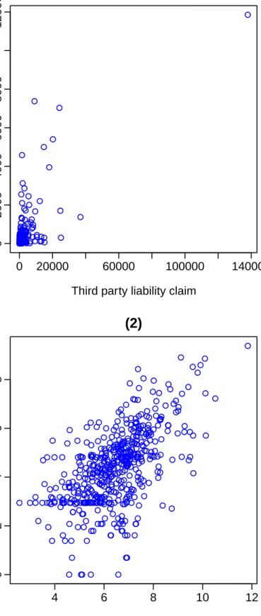
Figure 2 provides graphs for simulated chains based on univariate data, and Figure 3 presents graphs for simulated chains based on bivariate data. In each graph, we have provided the simulated chains for the bandwidth and transformation parameters. According to the SIF values presented in Table 1 and the graphs of the simulated chains presented in Figure 2, we found that the simulated chains of parameters for both variables have achieved very good mixing performance.
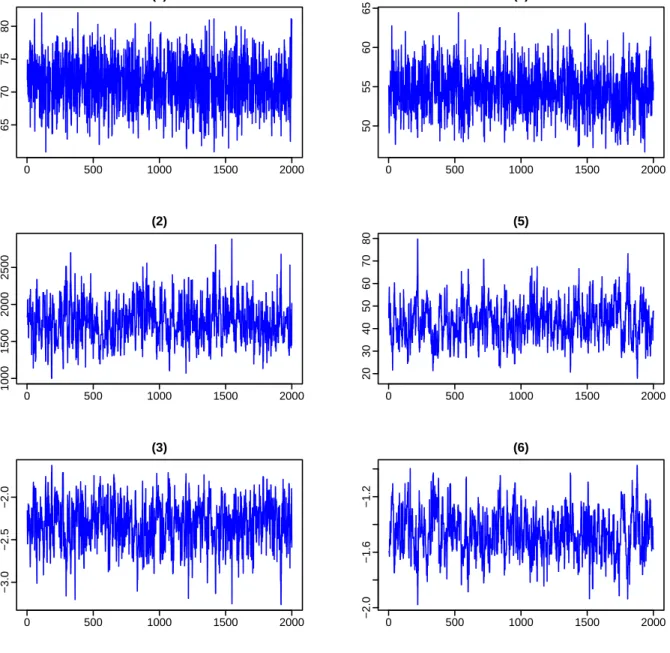
Table 2 and the graphs of the simulated chains presented in Figure 3 show that the simu-lated chains of parameters for the bivariate density estimator have achieved reasonable mixing performance. Even though the SIF values ofλ11 andλ21 are larger than those of the other
pa-rameters, they are well below 100, which is usually considered as a benchmark for a reasonable mixing performance. Therefore we could conclude that the inefficiency of the simulated Markov chains is tolerable in view of the number of iterations.
4.2 Accuracy of results obtained through the MCMC algorithms
In order to examine the performance of the MCMC algorithms for the estimation of bandwidth parameters and transformation parameters, we looked at a collection of descriptive statistics and compared our results with their empirical counterparts. We also compared the performance of our bandwidth selection methods with that of some other bandwidth selectors that have been widely used in the literature. The bandwidth parameters and transformation parameters were estimated or selected using the following methods.
• M1: MCMC algorithm based on univariate data;
• M2: MCMC algorithm based on bivariate data;
• R1: Rule-of-thumb discussed by Scott (1992) for bandwidth selection based on univariate data with transformation parameters estimated throughM1;
• R2: Rule-of-thumb for bandwidth selection based on univariate data with transformation
parameters estimated throughM2;
• N1: The normal reference rule for a diagonal bandwidth selection discussed by Bowman
and Azzalini (1997) with transformation parameters estimated throughM1;
• N2: The normal reference rule approach for a diagonal bandwidth selection with
trans-formation parameters estimated throughM2;
• P1: The direct plug-in approach for a diagonal bandwidth selection discussed by Sheather and Jones (1991) with transformation parameters estimated through M1; and
• P2: The direct plug-in approach for a diagonal bandwidth selection with transformation
parameters estimated throughM2.
Table 3 presents a summary of descriptive statistics calculated with different bandwidth and transformation parameters estimated via different methods. These descriptive statistics are the correlation coefficient, coefficient of variation (CV), mean, median and standard deviation (SD). We are particularly interested in the correlation calculated through the Bayesian sampling algorithms presented in Section 3.3.
First, the sample correlation coefficient betweenx1 andx2 is 0.73, indicating a very strong
positive correlation between the two variables. The correlation coefficient obtained throughM2
is 0.26, which is higher than the correlation coefficient obtained throughM1. This demonstrates
that the bivariate sampling algorithm captures the correlation betweenx1 and x2 better than
the univariate sampling algorithm being applied to each univariate variable separately. We then borrowed the results obtained from our bivariate sampling algorithm and replaced the band-widths with the above-mentioned other selectors and did a similar comparison. For all different bandwidth selectors that we examined, the bivariate density estimator using the transformation parameters estimated through the bivariate sampling algorithm can better capture the correla-tion betweenx1 and x2 than the transformation parameters estimated through the univariate
sampling algorithm.
Second, when we did a comparison of M1 with R1,N1 and P1 to examine the performance
of the univariate sampling algorithm, as well as a comparison of M2 with R2, N2 and P2 to
and normal reference rule clearly underestimate the mean values. Even though the direct plug-in approach discussed by Sheather and Jones (1991) performs better than the rule-of-thumb and normal reference rule, but the plug-in approach does not perform better than the univariate sampling algorithm for the mean level ofx1. Our univariate sampling algorithm and the direct plug-in approach provide similar results for the mean level of x2. Note that even though the performance ofP1 and P2 are reasonably good, they both used the estimates of transformation
parameters obtained through the univariate and bivariate sampling algorithms to derive the kernel density estimator via transformations.
Third, all bandwidth selectors perform pretty well in terms of calculating the median. How-ever, both the univariate and bivariate sampling algorithms and the direct plug-in approach perform better than the rule-of-thumb and normal reference rule.
Fourth, even though on average there is an improvement of 47% in capturing the correlation between x1 and x2 through the bivariate sampling algorithm against the univariate sampling algorithm, it seems that almost both algorithms tend to underestimate the correlation coeffi-cient indicated by the sample correlation coefficoeffi-cient. There are two possible reasons for this phenomenon. One is because the sampling algorithms were developed based on the Kullback-Leibler information criterion, which aims to minimise the discrepancy between the density estimator and the underlying true density. This criterion does not aim to only capture the correlation between the two variables. The other possible source of inaccuracy may come from the use of numerical approximations for the integrals and the double integral in the correlation formula given by (8).
5
Conclusions
This paper presents Bayesian sampling algorithms for estimating bandwidths and transforma-tion parameters in the kernel density estimatransforma-tion via transformatransforma-tions for bivariate data. The proposed sampling algorithms can estimate not only the bandwidth parameters but also the transformation parameters through a Metropolis-Hastings sampling procedure. Our sampling algorithms have achieved very good mixing performance. When estimating the density of bi-variate insurance claim data, we have found that our bibi-variate sampling algorithm has an improvement over what Bolance, Guillen and Nielsen (2008) did, where the transformation pa-rameters were estimated by dealing with each variable separately. We calculate the correlation
coefficient through our bivariate sampling algorithm in comparison with the correlation coeffi-cient calculated through the univariate sampling algorithm. We have found that the correlation is better captured via the bivariate sampling algorithm than the univariate sampling algorithm. We have also calculated a collection of descriptive statistics using parameters estimated through different methods. Our sampling algorithms clearly outperform the rule-of-thumb and normal reference rule for bandwidth selection, and are as good as the direct plug-in method.
We have also computed the conditional tail expectation as Bolance, Guillen and Nielsen (2008) did. However, our results tend to underestimate the empirical conditional tail expec-tations. This is not surprising because our sampling algorithms were developed based on the Kullback-Leibler information criterion, under which our results are optimal when we look at the entire density rather than the tails of the density. Further research could focus on finding the optimal bandwidth and transformation parameters for bivariate kernel density estimation via transformations, which give a more accurate estimate of the tail of the joint density.
References
[1] Bolance, C., Guillen, M., Nielsen, J.P., 2003. Kernel density estimation of actuarial loss functions, Insurance: Mathematics and Economics, 32, 19-36.
[2] Bolance, C., Guillen, M., Pelican, E., Vernic, R., 2008. Skewed bivariate models and non-parametric estimation for the CTE risk measure, Insurance: Mathematics and Economics, 43, 386-393.
[3] Buch-Larsen, T., Nielsen, J.P., Guillen, M., Bolance, C., 2005. Kernel density estimation for heavy-tailed distributions using the Champernowne transformation, Statistics, 39(6), 503-518.
[4] Clements, A.E., Hurn, A.S. and Lindsay, K.A., 2003. Mobius-like mappings and their use in kernel density estimation, Journal of the American Statistical Association, 98, 993-1000. [5] H¨ardle, W., 1991. Smoothing Techniques with Implementation in S, Springer-Verlag, New
York.
[6] Hjort, N.L., Glad, I.K., 1995. Nonparametric density estimation with a parametric start, The Annals of Statistics, 23, 882-904.
[7] Izenman, A.J., 1991. Recent developments in nonparametric density estimation, Journal of the American Statistical Association, 86, 205-224.
[8] Kim, S., Shephard, N., Chib, S., 1998. Stochastic volatility: Likelihood inference and comparison with ARCH models, Review of Economic Studies, 65, 361-393.
[9] Marron, J.S., 1988. Automatic smoothing parameter selection: A survey, Empirical Eco-nomics, 13, 187-208.
[10] Meyer, R., Yu, J., 2000. BUGS for a Bayesian analysis of stochastic volatility models, Econometrics Journal, 3, 198-215.
[11] Roberts, G.O., 1996. Markov chain concepts related to sampling algorithms. In: Gilks, W.R. Richardson, S., Spiegelhalter, D.J. (Eds.) Markov Chain Monte Carlo in Practice, Chapman & Hall, London, 45-57.
[12] Scott, D.W., 1992. Multivariate Density Estimation. Theory, Practice and Visualisation, John Wiley & Sons, Inc.
[13] Sheather, S.J., Jones, M.C., 1991. A reliable data-based bandwidth selection method for kernel density estimation, Journal of the Royal Statistical Society, Series B, 53, 683-690. [14] Simonoff, J.S., 1996.Smoothing Methods in Statistics, Springer, New York.
[15] Tse, Y.K., Zhang, X., Yu, J., 2004. Estimation of Hyperbolic Diffusion with Markov Chain Monte Carlo Simulation, Quantitative Finance, 4, 158-169.
[16] Wand, M.P., Marron, J.S., 1995.Kernel Smoothing, Chapman & Hall.
[17] Wand, M.P., Marron, J.S., Ruppert, D., 1991. Transformations in density estimation, Journal of the American Statistical Association, 86, 414, 343-353.
[18] Zhang, X., Brooks, R.D., King, M.L., 2009. A Bayesian approach to bandwidth selection for multivariate kernel regression with an application to state-price density estimation, Journal of Econometrics, 153, 21-32.
[19] Zhang, X., King, M.L., Hyndman R.J., 2006. A Bayesian approach to bandwidth selection for multivariate kernel density estimation, Computational Statistics & Data Analysis, 50, 3009-3031.
Table 1: MCMC results using univariate data
x1 Estimate SIF Acceptance rate x2 Estimate SIF Acceptance rate
h1 71.031 8.76 0.203 h2 54.467 19.91 0.256
λ11 1760.887 24.97 0.188 λ12 43.055 54.92 0.270
λ21 -2.302 22.58 0.238 λ22 -1.466 54.51 0.210
Table 2: MCMC results using bivariate data
x1 Estimate SIF Acceptance rate x2 Estimate SIF Acceptance rate
h1 124.138 6.78 0.299 h2 128.536 8.91 0.279
λ11 2234.750 67.93 0.225 λ12 51.741 30.96 0.291
λ21 -3.030 66.12 0.235 λ22 -0.814 28.57 0.257
Table 3: A summary of descriptive statistics obtained through different parameters estimated via different methods
ρ CV ofx1 CV ofx2 Mean ofx1 Mean ofx2 Median ofx1 Median ofx2 SD ofx1 SD ofx2
Empirical 0.73 3.76 3.04 1827.60 283.92 674.00 88.00 6867.82 863.17 M1 0.20 2.36 2.42 1530.29 176.52 677.09 86.31 3605.32 427.25 M2 0.26 1.94 2.79 1320.57 241.42 675.83 85.21 2566.95 684.10 R1 0.11 1.99 2.60 1168.44 143.26 662.69 82.45 2328.53 372.46 R2 0.18 1.61 2.85 1054.51 238.63 662.71 84.46 1693.41 680.82 N1 0.06 1.96 2.81 1063.43 121.70 651.85 76.08 2088.49 342.44 N2 0.10 1.58 2.99 954.33 235.37 651.85 80.92 1510.86 702.68 P1 0.27 2.30 2.48 1462.01 207.16 675.29 87.14 3359.27 514.43 P2 0.34 1.92 2.87 1305.34 270.60 675.38 87.24 2511.42 777.16
Figure 1: (1) Scatter plot of bodily injury claims versus third party liability claims; and (2) Scatter plot of logarithmic bodily injury claims versus logarithmic third party liability claims.
0 20000 60000 100000 140000 0 2000 4000 6000 8000 12000
(1)
Third party liability claim
Bodily injur y claim 4 6 8 10 12 0 2 4 6 8
(2)
Logarithm of third party liability claim
Logar
ithm of bodily injur
Figure 2: Plots of simulated chains based on univariate data series. The left column contains the simulated chains of (h, λ1, λ2) based on the first series, and the right column contains the
simulated chains of the same set of parameters based on the second series. In each of the six graphs, the horizontal axis represents the serial number of draws which retained one draw for every five draws; and the vertical axis represents parameters values.
0 500 1000 1500 2000 65 70 75 80 (1) 0 500 1000 1500 2000 50 55 60 65 (4) 0 500 1000 1500 2000 1000 1500 2000 2500 (2) 0 500 1000 1500 2000 20 30 40 50 60 70 80 (5) 0 500 1000 1500 2000 −3.0 −2.5 −2.0 (3) 0 500 1000 1500 2000 −2.0 −1.6 −1.2 (6)
Figure 3: Plots of simulated chains based on bivariate data series. The left column contains the simulated chains of (h, λ11, λ12), and the right column contains the simulated chains of
(h, λ21, λ22). In each of the six graphs, the horizontal axis represents the serial number of draws
which retained one draw for every five draws; and the vertical axis represents parameters values.
0 500 1000 1500 2000 115 120 125 130 135 (1) 0 500 1000 1500 2000 −4.0 −3.0 (2) 0 500 1000 1500 2000 1500 2500 3500 (3) 0 500 1000 1500 2000 120 125 130 135 140 (4) 0 500 1000 1500 2000 −1.1 −0.9 −0.7 −0.5 (5) 0 500 1000 1500 2000 30 40 50 60 70 80 90 (6)