Enlargement of Preferential Trade Areas: Essays on Trade Displacement
David L. Buehler
A dissertation submitted to the faculty of the University of North Carolina at Chapel Hill in partial fulfillment of the requirements for the degree of Doctor of Philosophy in the
Department of Economics.
Chapel Hill 2011
ii
iii
ABSTRACT
David L. Buehler: Enlargement of Preferential Trade Areas: Essays on Trade Displacement (Under the direction of Dr. Alfred Field)
Trade displacement effects caused by the enlargement of a preferential trade area are
examined in theory and empirically. The Ricardian model of trade is expanded to four
countries to show the trade and welfare effects on members and nonmembers caused by
enlargement of a customs union. A simulation follows to help clarify the results. The
enlargement of the European Union is examined through a dynamic shift-share analysis and
the gravity model is employed to determine the significance of trade displacement. The
analysis demonstrates that trade displacement is likely to have occurred with the enlargement
iv
ACKNOWLEDGMENTS
I am indebted to a number of people who have provided me with an immense amount
of support throughout the process of completing this work. I am especially grateful to my
wife, Christin, my son, Colton, my parents, Larry and Carla Buehler, and all of my other
family and friends who have granted me their patience and support. In addition, I would like
to thank my advisor, Dr. Al Field, for all of his guidance, along with rest of my dissertation
committee and the faculties at the University of North Carolina Chapel Hill, West Virginia
v
TABLE OF CONTENTS
LIST OF TABLES ... vii
LIST OF FIGURES ... ix
DISSERTATION INTRODUCTION ...1
CHAPTER I. Trade Displacement in Theory: Evidence from the Ricardian Model ...3
Introduction ...3
Literature Review...4
The Four-Country Ricardian Model with a Continuum of Goods ...11
Numerical Simulation ...35
Policy Implications and Conclusions ...50
II. Trade Displacement: Empirical Evidence from a Shift-Share Analysis of the EU ...63
Introduction ...63
Methodology ...65
Data ...71
Analysis by Country Group ...73
Analysis by Individual Countries...82
Policy Implications ...93
Conclusions ...95
vi
Introduction ...98
Literature Review...100
Data ...101
Model ...102
Descriptive Statistics ...106
Results ...109
Conclusions ...125
APPENDICIES ...127
vii
LIST OF TABLES
Table
1.1 Two country simulation ...52
1.2 Three country simulation ...53
1.3 Four country simulation ...54
1.4 Four country model; Two Country Unions ...56
1.5 Four country model; Union Enlargement Possibilities ...57
1.6 Four country case, different endowments ...58
1.7 Union enlargements, different endowments ...62
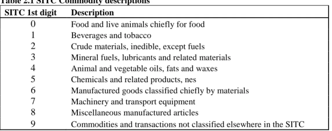
2.1 SITC Commodity descriptions ...71
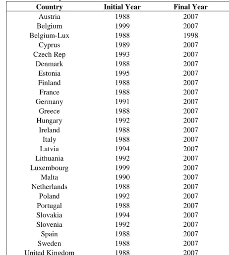
2.2 Data Availability ...72
2.3 Percentage growths from 1993-5 average to 2004-6 average ...79
2.4 Trends in share of European exports ...85
2.5 Expected results of trade effects ...95
3.1 OLS estimates of γ ...110
3.2 OLS estimates of λ ...112
3.3 OLS estimates of ,− , ...112
3.4 OLS estimates of γ ...115
3.5 OLS estimates of λ ...116
3.6 OLS estimates of ,− , ...117
3.7 SUR estimates of γ ...120
3.8 SUR estimates of λ ...121
viii
3.10 Tests of equality across all six equations of SUR
for standard gravity model variables ...122
3.11 Test of equality of estimated coefficients of
distance variable for each pair of countries ...122
3.12 Test of equality across all six equations of SUR
ix
LIST OF FIGURES
Figure
1.1 Two country Ricardian model ...9
1.2 Three country Ricardian model ...11
1.3 Trade pattern for four country, free trade case ...17
1.4 Trade pattern for four country, tariff case ...23
2.1 Nominal Total Trade ...75
2.2 Share of Total Trade by Country Groups ...76
2.3 Percentage growth in trade ...77
2.4 Competitiveness Effect ...78
2.5 Nominal Growth in Exports ...80
2.6 Nominal Values of Competitiveness Effect ...81
2.7 Share of EU Exports ...83
2.8 Competiveness Effects, by growth rate ...86
2.9 Average Annual Competitiveness Effect, by growth rate ...89
2.10 Nominal values of competitiveness effects...90
3.1 2008 Nominal value of imports of selected EU countries ...106
3.2 Share of country imports ...108
DISSERTATION INTRODUCTION
The following collection of essays addresses the concept of trade displacement in
international trade. While the terms ‘trade creation’ and ‘trade diversion’ have existed since
the 1950’s as part of the discussion of the trade effects of a customs union or preferential
trade agreement, trade displacement has received less attention in the international trade
literature. Trade displacement occurs when an existing customs union expands to include
new members and entails former members’ trade being displaced by the new members. Each
of the following essays addresses this effect in different ways.
Trade displacement is first outlined in theory, using a Ricardian trade model adapted
to four countries. Using the Dornbusch, Fischer, and Samuelson model of two-country trade
and the Appleyard, Conway, and Field three-country model as a foundation, the Ricardian
model is expanded to four countries in order to examine the possible enlargement of an
existing customs union. A fourth country is needed as there must exist a customs union (of at
least two countries), an acceding country, and a country not included in the union. This
process of enlargement allows the identification of trade creation, trade diversion, and trade
displacement as a result. After the general equilibrium model is presented, a numerical
simulation is presented, which allows a clearer picture of the various effects. Welfare
analysis in the theory and simulation also demonstrate the potential welfare effects of the
enlargement process.
The second chapter examines the export performance of the European countries over
2
EU members exports to the existing members are taking the place of members’ exports to
other members. Using a shift-share analysis, export performance is examined after
accounting for various other factors, including growth of world trade and market conditions.
The analysis shows that the new EU members’ exports to the EU have increased fairly
dramatically through the sample. Conversely, some of the existing members’ exports to EU
countries have decreased over the same time period.
Rather than using export data, the final chapter examines import data to attempt to
determine the existence of trade displacement. In terms of imports, trade displacement
occurs when a member of the customs union begins to import goods from a new member
instead of an existing member. The gravity model is employed to estimate the effects on
trade from the different country groups – core members, other members, new members, and
the rest of the world. More importantly, the changes in these estimates from one period to
the next are used to determine the changing nature of trade from the groups to the large EU
countries. Some evidence of trade displacement is presented, as the estimation shows
increases in imports from the new members combined with decreases or smaller increases in
CHAPTER 1
Trade Displacement in Theory: Evidence from the Ricardian Model
I. Introduction
There has been much theoretical work on the role of integration in international trade,
but there has been relatively less work examining the growth of such trade agreements. This
paper will further develop the theoretical framework of international trade based on a
Ricardian model as presented by Dornbusch, Fischer, and Samuelson (DFS), and later
Appleyard, Conway, and Field (ACF). The DFS model outlines the two-country model, and
the ACF work extends the framework to three countries, which allows for the examination of
different trade agreements between trade partners. This paper adds a fourth country while
utilizing the same theoretical framework. The reason for this addition of a fourth country is
to add the ability to consider countries potentially joining an existing trade agreement while
others remain outside of the agreement. With the addition of a fourth country to the model,
this paper will also focus on the theoretical possibility of trade displacement occurring with
the enlargement of a preferential trade agreement, in addition to trade creation and trade
diversion as outlined by previous literature.
Differing models of international trade suggest that the degree of similarity between
partners has an effect of the gains (and costs) of economic integration. In the Ricardian
model, as evidenced by ACF, economic integration is most beneficial to those countries that
are most dissimilar. But while the three country model is capable of examining the different
4
effects of potential enlargement of the area of integration on the current members and the
remaining countries. This four-country model allows for this investigation into the
enlargement of an area of integration in terms of trade effects and welfare analysis, with a
focus on trade creation, trade diversion, and trade displacement. The model also permits
comparison of potential accession countries, suggesting that current members could have
different notions of which non-member should be allowed to integrate. The model is
examined with the enlargement of the European Union in mind, though it is presented more
generally and is thus not restricted to that particular setting. Ultimately, this paper seeks to
answer the questions of how enlargement affects the welfare of current members of a
customs union, the acceding country, and those not acceding.
The paper is presented as follows: Section 2 of the paper briefly presents existing literature
on the subject. The third section outlines the model used for analysis. A brief description of
the model and results from the two-country and three-country models is included before
more detail is presented for the country case. Section 4 presents the results of the
four-country model simulation, including a welfare analysis of the enlargement process. Section 5
concludes.
II. Literature Review
A. Overview
The literature relating to the topics of trade creation, trade diversion, and trade
displacement within the Ricardian model will be discussed in the following groups: general
theoretical models of customs union1, work testing for evidence of the three effects, and previous versions of the Ricardian model. The latter will be discussed in separate sections
immediately following this section.
5
Discussion of literature on customs unions theory begins with Jacob Viner’s work
The Customs Union Issue in 1950, in which Viner first outlines the terms trade creation and
trade diversion. Viner’s work focused on the welfare effects of the creation of a customs
union, and, as a general result, found trade creation – the movement of production from a
high cost location to a lower cost location – to have a positive effect on global welfare, while
trade diversion – the movement of production from a low cost producer to a high cost
producer – has a negative effect on global welfare. Viner’s work inspired a series of
literature in the 1950’s including, but certainly not limited to, the works of James Meade,
Franz Gehrels, and Richard Lipsey. One of the main contributions of Lipsey’s work included
the positive and negative consumption effects of customs union formation along with the
production effects.
These early works sparked debate to the merit and effectiveness of customs unions
and preferential trade agreements. Much of the policy debate centered around the choice of
partners for a preferential trade agreement. On opposite sides of one point of contention
were Wonnacott and Lutz (1989) and Summers (1991), who suggested that large initial trade
flows between potential PTA members would lead to a positive effect, as trade creation
outweighed trade diversion. Bhagwati and Panagariya (1996) disputed this result, showing
that high initial trade volumes do not necessarily suggest positive welfare effects for the
member countries. The debate continues today, with Eicher, Henn, and Papageorgiou (2008)
“revisiting” the issue.
Kemp and Wan’s (1976) work included the next significant theoretical outcome, as
the authors demonstrated that one could always construct a welfare-improving customs union
6
Much like Viner’s work, this theory sparked a series of policy debates, as an important aspect
of the Kemp-Wan conclusion relies on the reduction of the common external tariff of the
customs union.
The above list of works includes major contributions to the literature regarding
customs unions. However, many include only a discussion of the formation of customs
unions or preferential trade agreements, and hardly touch on the subject of the enlargement
of such an area. One example that does briefly discuss this topic is Ronald Wonnacott’s
1996 paper, in which the author mentions that the expansion of a customs union will reverse
trade diversion caused by the initial formation of the union. However, Wonnacott does not
get into the details of the theory of this process as I attempt to. Welfare effects of a joining
nation have been sparsely addressed, with Williams (1972) leading the way. I aim to
examine the effects of the enlargement of a customs union – in terms of trade creation,
diversion, and displacement – on initial members of a customs union, a joining member, as
well as those not joining the customs union. While the ideas of trade creation and trade
diversion have existed in the literature since Viner, the theoretical literature on trade
displacement is far more insubstantial.
Attempts to empirically isolate the effects of trade creation and trade diversion
typically involve the examination of one particular regional integration and/or one particular
sector of trade. Few, however, address the issue of an expanding customs union or
preferential trade agreement, and thus, few explore the significance of trade displacement
effects of such an enlargement. The work in this area is more recent, with Wilhelmsson
(2006) examining the trade displacement effects of the expanding EU, and Fratianni and Oh
7
the gravity model to test the effects. Wilhelmsson, in particular, specifically addresses the
trade displacement effect through enlargement.
Extensions of the Dornbusch, Fischer, and Samuelson (DFS) version of the Ricardian
trade model are not new, but have also not lost influence or importance. Various scholars
continue to use the model as a basis for examination of various issues in international trade.
More recent examples of the extensions of the model include several papers by Kiminori
Matsuyama (2006), and the model also serves as the foundation for recent additions to
international trade literature by John Romalis (2004). Matsuyama has expanded the
Ricardian model (and more specifically, the DFS model) in several different ways, including
examining the inclusion of multiple factors and technologies dependent on destination (home
or foreign), and also different demand preferences than the DFS model. Romalis’ model is
more along the lines of the Heckscher-Ohlin variety and addresses factor proportions and
their role in trade, but the basis of the model begins with the DFS model.2 Other recent examples of DFS extensions include Eaton and Kortum (2002) and Alvarez and Lucas, Jr.
(2006), which examine the role of geography in trade, as well as those of country size and
tariff policy.
Incorporating the modifications of these various authors into the discussion of
regional integration would without doubt prove valuable as well. Building off the original
DFS model and addressing regional integration in the same manner as ACF, I will
complement these various extensions of the Ricardian models by specifically addressing the
enlargement of regional integration. Before doing so, a brief review of the Ricardian model
with a continuum of goods in the two and three country settings is presented.
2
8
B. The two-country Ricardian Model with a continuum of goods
The Ricardian model with two countries and a continuum of goods, as outlined by
Dornbusch, Fischer, and Samuelson (DFS), determines the competitive margin between
exported and imported goods. The model assumes constant unit labor requirements
(Assumption 1) for all (n) commodities in both Country 1 and Country 2 (a1i and a2i; where i
represents any good in the continuum). The commodities are indexed so that they are ranked
in order of diminishing comparative advantage for country 1, that is
(1)
> ⋯ >
> ⋯ >
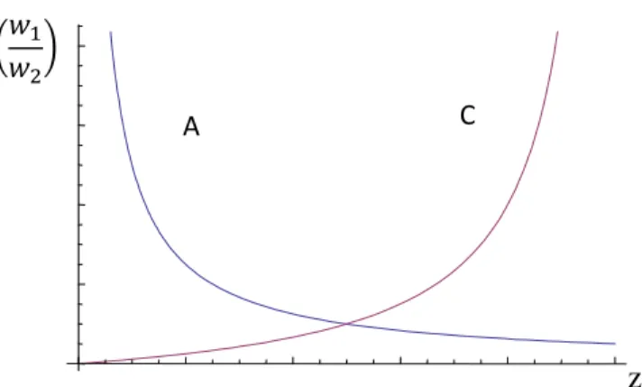
In figure 1.1, this system of indexing, along with the wages in each country, produces the A
curve, which draws the export incentive condition. Along the A curve, Country 1 is
indifferent between producing the good at home, costing a1iw1, or importing the good from
Country 2, costing a2iw2 (given the absence of transportation costs and trade barriers, and
assuming an exchange rate of 1). To the left of the A curve, Country 1 has a comparative
cost advantage, producing those goods at home for consumption as well as exporting them to
Country 2. Similarly, for those goods to the right of the A curve, Country 2 has a
comparative cost advantage, and Country 1 chooses to import these goods.
a1iw1< a2iw2 left of the A curve
a1iw1 = a2iw2 along the A curve
a1iw1> a2iw2 right of the A curve
The other major determinants in the DFS general equilibrium are the assumptions of identical
demands across countries and balanced trade, given by the equation
(2)
9
whererepresents the cumulative percentage of income spent on goods through zi. Using
= 1 − and rewriting, we have
(3)
=
1 −
The intersection of the cost advantage curve (A curve) and the balanced trade curve (C
curve) results in the equilibrium wage ratio
∗
and the crossover good z*. At the
equilibrium wage ratio, Country 1 produces and exports all goods closer to the origin than z*,
while it imports all goods further from the origin than z*.
Figure 1.1 – Two country Ricardian model
z
Adding tariffs to the two country model creates a third area of non-traded goods apart from
exports and imports only as in the free trade case. With tariffs in place on imports
(reciprocally by both countries), there exists certain goods which Country 1 produces for
consumption but does not export. Likewise is true for Country 2. These two cases (two
country free trade and two country tariff case) will be examined further using a simulation
later in the paper. An important note is that the authors of the DFS paper explore several
other scenarios outside of the tariff case in the two country setting. While not critical to the
A
10
question at hand, they each have important implications and the reader should find detailed
explanations in the original DFS paper.
C. The three-country Ricardian model with a continuum of goods
The expansion to three countries, as presented by Appleyard, Conway, and Field
(ACF), allows for examination of the effects of trade agreements between pairs of countries.
The model is built in a similar fashion to the two country model, indexing the continuum of
goods between 0 and 1, and decreasing in terms of country 1’s comparative advantage.
However, it is important to note that there are essentially two A curves, with
A2(z)=a2(z)/a1(z) and A3(z)=a3(z)/a1(z), that map out cost advantages with the respective
wage ratios. Combining the comparative cost advantages and a balanced trade restriction, we
again see that each country specializes in the production of a set of goods and exports these
goods in exchange for each of the other countries’ goods. The crossover goods, of which
there are two in the three-country setting, are determined by the indexed good where it is
cheaper to produce it in country 2 than in country 1 (z1*) and the indexed good where it is
cheaper to produce it in country 3 than in country 2 (z2*). Figure 1.2 shows the equilibrium
for the three-country, free trade case for a general production function. The introduction of
tariffs again creates sets of goods (two of them) that are produced for home consumption but
not traded.
The introduction of the third country allows, among other things, the analysis of trade
agreements between certain members. The policies of one or more countries have effects on
the direction of trade, the terms of trade, and the welfare of all three nations (the entire world
in this case). However, in the three country model, enlargement of a trade agreement to
11
be a member of the union. A fourth country is needed to analyze countries not included in
the enlargement process.
Figure 1.23 - Three country Ricardian model
III. The four-country Ricardian model with a continuum of goods
A. General Model / Free trade
Four countries are denoted Ci, with i = 1, 2, 3, or 4. An arrayed number of goods are
produced (and consumed) and each good is positioned along the continuum [0,1] by variable
z.4 Following ACF, the following assumptions are made about technology, which shows
through the labor-output ratio ai(z). For Ai(z)=ai(z)/a1(z):
3
In the three-country free trade case, there are four equations that must be satisfied: two (binding) export conditions and two balanced trade equations. In the figure, the export condition for C1, which determines z1*,
has been substituted into the other three equations, and those equations are represented by the three planes in the figure. The intersection of the three planes represents the general equilibrium of z1*, z2*, and (w1/w3)*.
(w1/w2)* = A2(z1*) is not represented in the figure.
12
(4)
! =α < 0
(5) $
$! =α % < 0
(6) &
&! =α ' < 0
(7) α' <α% <α < 0
The first assumption is a standard assumption in the two-country case ensuring the ability to
order the commodities in terms of comparative advantage. Adding Assumptions 2-4 ensures
that Ai(z)/Aj(z) is increasing in z for j≤i. All together, the assumptions mean that
comparative advantage, as z increases, shifts toward countries with a higher i under the
assumption that national skill level increases from C1 to C2 to C3 and to C4.5
Countries will import a good from another country if it is more expensive to produce it at
home, and likewise, they will have a comparative advantage and export goods for which the
country is the lowest-cost producer6. For i = 2,3,4, define the wage ratio Ωi = w1/wi. Then
country i will export goods z for which the following holds for j ≠ i:
(8) ( ≤ **
5 See ACF (1989) for example of production involving skill-based technology. 6
With costs of production of aiwi in each respective country, there is an implicit assumption that every good on
13
The parameter e represents the international exchange rate.7
These descriptions of comparative advantage define crossover goods z1, z2, and z3,
given by the following equations:
(9) Ω = +,-.
(10)
Ω
Ω% = /
+,-. +%,-.0
(11) ΩΩ%
' = / +%,-%. +',-%.0
For values below z1, country 1 produces and exports to all three trading partners. Likewise,
country 2 produces goods between z1 and z2 and exports to all three partners. For goods
between z2 and z3, country 3 is the exporter, and for goods above z3, country 4 is the
exporter.
At this moment, it is important to note the role that the Ω’s play in this model.
Changes in these real wage ratios have an impact on the location in the continuum of the
crossover good. As ACF (1989) states, “The real wage ratios can be interpreted as
trade-weighted averages of the commodity terms of trade.” Hence, when we get away from a free
trade situation, policy (tariffs) will not only play a direct role in affecting the location of
crossover goods and thus the pattern of trade, but also have an indirect effect through the
terms of trade. This is an important note, as partial equilibrium models often ignore this
indirect effect. These effects will become clearer in the next example.
The fact that the wage ratios, combined with the unit labor costs, determine the prices
of the goods produced demonstrates the perfectly competitive nature of the model. Perfect
7
14
competition in the labor markets implies constant wages across the different industries (but
not across countries). As far as the output markets, the prices of the goods are determined by
the wages and technology, implying perfectly competitive output markets as well – resulting
in the continuum of goods being dubbed a ‘continuum of competitive industries’8 as well.
Foreign goods and domestic goods are perfect substitutes, as consumers decide where to
purchase goods from based solely on price, and the production results in marginal cost
pricing of the goods. Full employment is an additional assumption that is also included in
the model.
Conway (2001) is one example of the DFS model extended with relaxed assumptions
in the industrial organization. A Ricardo-Viner (RV) model is introduced in comparison to
the more traditional DFS model, and firms earn positive profits in this imperfectly
competitive model. Some of the important results of this alternate assumption include home
wages that are dependent on foreign wages and firms from each country capturing profits
according to the difference in relative productivity. Conway also examines an alternative to
the full employment assumption. Results of this comparison show the importance of the
perfect competition assumption, as the imperfectly competitive RV model demonstrates
opposite results from the DFS model in the case of movement of the z values – a critical
aspect of the examination of trade policy shocks in the DFS framework.
Following both ACF and DFS using a Mill demand construction, the per capita welfare
function of country i is
(12)
1 = 2 3
4 ,-.
5,6.7-/
15
where Li is the labor force of country iand Ei(z) is the real expenditure on good z in country i.
Expenditure on each commodity is a constant share b(z) of total expenditure and is identical
across countries. The function b(z) is assumed to be strictly positive, and integration on the
continuum of goods (for 0 to 1) results in unity. Hence, the demand side of the model
follows the traditional, uniform homothetic DFS assumptions that all consumers have
identical Cobb-Douglas preferences over the continuum of goods and implies that the
fraction of expenditure spent on a subset of goods is θ(zi) and is defined by the equation:
(13)
,-. = 2
9,-.7-6:
4 > 0
Matsuyama (2000) and Stibora and de Vaal and (2007) demonstrate the results of relaxing
these assumptions of the traditional DFS model. By altering the continuum of goods such
that higher income household purchase a larger variety of goods (which can be interpreted as
necessity and luxury goods), the introduction of non-homothetic preferences demonstrates
that within-country income distributions will affect the import and export equilibrium values.
Returning to the traditional assumption of homothetic preferences, trade balance conditions
are also needed in this equilibrium model, and these represent the simultaneous demand of all
countries. Trade balances in the form of imports set to equal exports are given in equations
14 through 17.9
(14) ;1 − ,-.< = ,-.;+ %%+ ''<
(15) ;,-. + ,1 − ,-..< = ,,-. − ,-..;+ %% + ''<
9
16
(16) ;,-. + ,1 − ,-%..<%% = ,,-%. − ,-..;+ + ''<
(17) ,-%.'' = ,1 − ,-%..;+ + %%<
Defining li = Li/L1 and simplifying our notation with:
(18)
= ,-.
we can give normalized trade balance equations in the form:
(19) 1 = >1 + ?
Ω+
?%
Ω% +
?' Ω'@
(20) 1 = , − . >1 +Ω?
+
?% Ω%
Ω
? + ?' Ω'
Ω
?@
(21) 1 = ,%− . >1 +Ω?%
% + ?
Ω
Ω%
?% +Ω?'' Ω%
?%@
(23) 1 = ,1 − %. >1 +Ω?'
' + ?
Ω
Ω'
?' + ?% Ω%
Ω'
?'@
The equations defining the crossover goods (14-17) combined with the balanced trade
equations (19-23) define independent relationships between the variables z1, z2, z3, Ω2, Ω3,
and Ω4. The implicit function theorem allows a joint solution of the six endogenous variables
17 A-
A? < 0,
A- A?% < 0,
A- A?' < 0, A-
A? > 0,
A- A?% < 0,
A- A?' < 0, A-%
A? > 0,
A-% A?% > 0,
A-% A?' < 0, A-
A? > 0, A-A?% < 0, A-A?' < 0, AΩ
A? > 0,
AΩ
A?% > 0,
AΩ
A?' > 0, AΩ%
A? ?, AΩ%
A?% > 0,
AΩ%
A?' ?, AΩ'
A? ?,
AΩ'
A?% ?,
AΩ'
A?' > 0,
Before introducing tariffs into the model, a common misconception about the continuum of
goods needs to be addressed. The four-country free trade model results in a trade pattern
illustrated by figure 1.3, with each country specializing in the goods in their respective region
of the continuum.10
Figure 1.3 – Trade pattern for four country free trade
The Ricardian model is sometimes criticized because it lacks intra-industry trade, and
there is little empirical evidence that supports complete specialization. These criticisms
spawned several new theories of international trade, including, but certainly not limited to,
10
C1 exports [0,z1] to the other three countries. Likewise, C2 exports [z1,z2], C3 exports [z2,z3] and C4 exports
[z3,1]. The figure is not to scale, and the size of the respective regions is determined by other parameters in the
18
Krugman’s model which specifically addressed intra-industry trade. However, the notion of
complete specialization in this Ricardian model with a continuum of goods can include
intra-industry trade.
In this model, complete specialization only implies that a country produces only the
goods which it can produce at a lower cost than any other country. However, it does not
imply that two countries cannot produce the same type of good. By the construction of the
model and the indexing of goods along the continuum from 0 to 1, there is no restriction that
two goods from the same industry must be at the same point on the continuum. It is certainly
possible for one good from an industry to be indexed at a different point than another good
from the same industry. For example, one type of automobile may be indexed very close to
0, meaning it lies in the region in which C1 is likely to have a comparative cost advantage.
Another type of automobile may lie closer to 1 on the index, implying a C1 comparative cost
disadvantage. C1 is therefore likely to export the first type of automobile, while it is likely to
import the second. The ability to include intra-industry trade in the model is a result of the
level of disaggregation of the goods along the continuum. If the goods are sufficiently
disaggregated, then slightly different goods, which might normally be considered from the
same industry, will be represented at different points on the continuum. In fact, as long as
the goods are more disaggregated than the level of aggregation that the term ‘industry’
implies, then the model can include this type of trade. Hence, from this point on, we will
assume that the goods in production (all goods produced in the world), are at a minimum
level of disaggregation as to include intra-industry trade.
An example of this disaggregation would be the difference between the various levels
19
Classification (SITC). The level of product homogeneity is very different and more
homogenous at the SITC digit level than at the SITC 1-digit level. Therefore, at the
4-digit level, it is more likely that two products with different SITC classifications may be part
of the same ‘industry’ and could be represented at two different points on the continuum.
For example, comparing apples (SITC 0574) to oranges (SITC 0571), it’s likely that a
country would have different cost advantages in their production resulting in different places
along the continuum of goods. However, both could easily be considered part of the same
industry of fruits and vegetables (SITC 05). It should be noted that, through the modification
to imperfect competition, Krugman’s model allows for intra-industry trade regardless of the
level of disaggregation that the term ‘industry’ implies.
This description of the disaggregation needed is an important distinction in this model
and has important implications in the interpretation of product specialization and trade
patterns. For one, the Ricardian model does not restrict intra-industry trade, so the notion of
complete specialization only implies production of goods for which a country has a
comparative advantage, but not the production of goods from a limited subset of all
industries. Second, the expansion (contraction) of region of the continuum that a country
exports means that a country does produce a greater (smaller) variety of goods, but it also
implies that the volume of trade increases (decreases).
B. Introduction of tariffs
Straying from the free trade model, we can form a similar, more general model with
each country levying a tariff on the other three trading partners. The tariffs are assumed to
take the form of a uniform ad valorem tariff on all imports coming into the country. Define
20
(24) D* = ,1 + E*.
Such tariffs will impact the pattern of trade as well as the real wage ratios, or the terms of
trade, as demand shifts due to the changes in prices (with tariffs). Countries will now import
from the producer with the cheapest tariff-inclusive price. For k ≠ i (k = j is permissible, but
τjj = 1), country i will export to country j if and only if
(25) D* ≤ D*FFF
For each potential trade partner, three inequalities must hold. Consider, for example, country
1’s exports to country 2. The exports from country 1 to 2, tariff inclusive, must be cheaper
than country 2 producing at home, so τ21a1w1≤a2w2. In addition, exports from country 1 to 2
must be cheaper, tariff inclusive, than exports from country 3 or 4, so τ21a1w1≤τ23a3w3 and
τ21a1w1≤τ24a4w4. Hence, with four countries, three partners each, and three inequalities,
there are a total of 36 inequalities. Of these inequalities, twelve are binding and define
twelve crossover goods. However, in some cases, which inequality is binding will be
determined by the level of tariffs. For example, examine z8, which determines the good that
is as cheap to produce at home in C2 as it is to import from C3. But if τ23 is significantly
more than τ24, then there might not exist any goods that are cheaper for C2 to import from C3
rather than C4. The crossover goods are defined by equations 26 to 37, along with the other
inequalities that need to hold. The inequality in bold type is the binding inequality when
tariffs are equal and not prohibitive.
(26a, 26b, 26c)
21
(27a, 27b, 27c)
GNIJH≤ GNHKH,LH.; D%Ω% ≤ +%,-. ; D%Ω' ≤ D%'+',-.
(28a, 28b, 28c)
GOIJH≤ GOHKH,LN. ; D'Ω% ≤ D'%+%,-%. ; D'Ω' ≤ +',-%.
(29a, 29b, 29c)
GIHKH,LO. ≤ JH ; D/++,-'.
%,-'.0 ≤ D%
Ω
Ω% ; D/
+,-'.
+',-'.0 ≤ D'
Ω
Ω'
(30a, 30b, 30c)
D%+,-P. ≤ΩD% ; GNH/KH,LQ.
KN,LQ.0 ≤ JH
JN ; D%/++',-,-PP..0 ≤ D%'
Ω
Ω'
(31a, 31b, 31c)
D'+,-R. ≤ΩD' ; GOH/KKH,LS.
N,LS.0 ≤ GON JH
JN ; D'/
+,-R. +',-R.0 ≤
Ω
Ω'
(32a, 32b, 32c)
D%+%,-T. ≤Ω% ; GIN/KN,LU.
KH,LU.0 ≤ GIH JN
JH ; D%/
+%,-T.
+',-T.0 ≤ D' Ω% Ω'
(33a, 33b, 33c)
D%+%,-V. ≤ DΩ% ; GHN/KN,LW.
KH,LW.0 ≤ JN
JH ; D%/++%',-,-VV..0 ≤ D' Ω% Ω'
(34a, 34b, 34c)
D'%+%,-X. ≤ D'Ω% ; D'%/++%,-X.
,-X.0 ≤ D' Ω%
Ω ; GON/
KN,LY. KO,LY.0 ≤
JN JO
(35a, 35b, 35c)
D'+',-4. ≤Ω' ; D'/++',-4.
,-4.0 ≤ D
Ω'
Ω ; GIO/
KO,LIZ.
22
(36a, 36b, 36c)
D'+',-. ≤ DΩ' ; D'/+',-.
+,-.0 ≤
Ω'
Ω ; GHO/
KO,LII.
KN,LII.0 ≤ GHN JO JN
(37a, 37b, 37c)
D%'+',-. ≤ D%Ω' ; D%'/+',-.
+,-.0 ≤ D% Ω'
Ω ; GNO/
KO,LIH. KN,LIH.0 ≤
JO JN
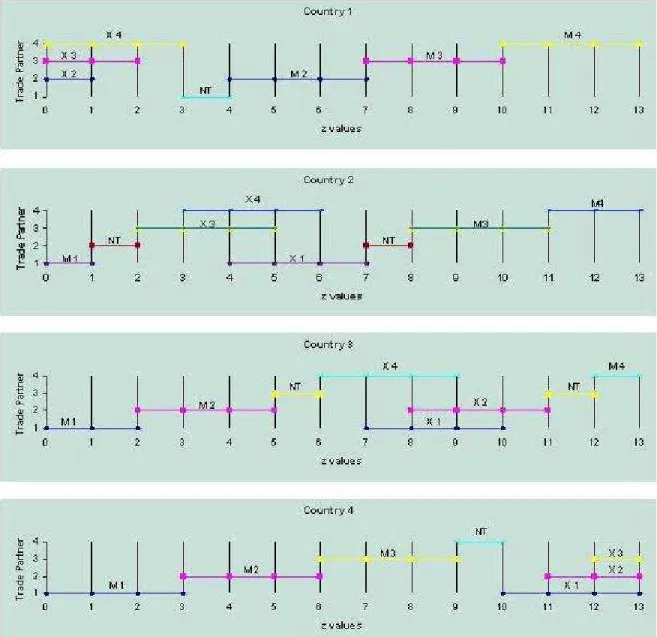
The resulting trade patterns are indicated in Figure 1.4.11,12 A few important notes are
needed. Each country continues to produce in the general region of the continuum as in the
free trade example; that is, country 1 produces the goods with low z values, while country 4
produces those goods with high z values. The tariffs have also caused a region of non-traded
goods for each country. Comparison to the free trade example also lends itself to interesting
outcomes. With each τ = 1, then z1 = z2 = z3 = z4. Likewise for zi for i = 5, 6, 7, and 8 or i =
9, 10, 11, 12.
11 There is potential for z
i< zi+1, but that is not necessarily a problem. Some z values may cross over one
another, while others can not. In general, z values can not cross over if doing so results in a country both importing and exporting a good. If this occurs, then the binding inequality is not the correct one of the three export conditions. Correcting the binding inequality will disallow both importing and exporting the same goods.
12 Please note that a z
23
The tariff-inclusive per capita welfare functions are
(26)
1 = 2 [9,-.
,-.\ 5,6. 6&
4 7- + 2 [
9,-.]
,-.D\ 5,6. 6^
6&
7- + 2 [9,-.]%
%,-.D%\ 5,6. 6 _
6^
7-+ 2 >9,-.]' ',-.D'@
5,6.
6 _
24
(27)
1 = 2 >] 9,-. ,-.D@
5,6. 6
4 7- + 2 >
9,-. ,-.@
5,6. 6`
6 7- + 2 >
9,-.]% ]%,-.D%@
5,6. 6
6`
7-+ 2 >]9,-.]' ',-.D'@
5,6.
6
7-(28)
1% = 2 >] 9,-. %,-.D%@
5,6. 6
4 7- + 2 >
]9,-. ]%,-.D%@
5,6. 6a
6
7- + 2 >9,-. %,-.@
5,6. 6
6a
7-+ 2 >]9,-.]' %',-.D%'@
5,6.
6
7-(29)
1' = 2 >] 9,-. ',-.D'@
5,6. 6$
4 7- + 2 >
]9,-. ]',-.D'@
5,6. 6b
6$
7- + 2 >]9,-.]% '%,-.D'%@
5,6. 6c
6b
7-+ 2 >9,-. ',-.@
5,6.
6c
7-which include the optimal demand condition for country i of Ei(zk)/Li = b(zk)wi/Pi(zk) for all
k and the constant returns pricing condition Pi(zk) = aj(zk)wjτij for all goods zk produced in
country j, for j = 1,2,3, or 4 (recall, if i=j, then τij =1). The consumer faces the
tariff-inclusive cost of production of the country with comparative advantage.
Trade balance equations are again needed, and the normalized equations are:13,14
13
As noted earlier, only three of the four countries are required. Country 3 is omitted.
25
(30) 1 =θ l
Ω+θ
l% Ω%+θ%
l' Ω'+θ'
(31) 1 = ,θT−θ'.Ω
l + ,θR−θ%. l ' Ω'
Ω
l + ,θP−θ. l % Ω%
Ω
l + ,θV−θ.
(32) 1 = ,1 −θ. l%
Ω% Ω'
l' + ,1 −θ. l
Ω
Ω'
l' + ,1 −θ4. Ω'
l' + ,1 −θX.
As we approach policy or tariff reform, we are interested in the effects on the trade
patterns of changes in tariffs. The changes in the position of the crossover goods are given
by equations 33 to 44. Recall that by the assumptions outlined, α2< 0, α2 – α3> 0, and α3 –
α4> 0. The direct impact of tariff reduction is much clearer, as an increase or decrease in the
z value of a crossover good will affect the exports and imports of countries on either side of
the good.
(33) zf = α1
,τ̂+Ωh.
(34) zf = α1
,τ̂%−τ̂%+Ωh.
(35) zf% = α1
,τ̂'−τ̂'+Ωh.
(36) zf' = α1
,−τ̂+Ωh.
(37) zfP = α 1
26
(38) zfR = α 1
−α% ,τ̂'%−τ̂'+Ωh−Ωh%.
(39) zfT = α 1
−α% ,τ̂%−τ̂+Ωh−Ωh%.
(40) zfV = α 1
−α% ,τ̂%+Ωh−Ωh%.
(41) zfX = α 1
%−α' ,−τ̂'%+Ωh%−Ωh'.
(42) zf4= α 1
%−α' ,τ̂'−τ̂%+Ωh% −Ωh'.
(43)
zf = α 1
% −α' ,τ̂'−τ̂%+Ωh%−Ωh'.
(44)
zf= α 1
%−α' ,τ̂%'+Ωh%−Ωh'.
It is also clear that the changes in the real wage ratios have an effect on the location of
a crossover good in the continuum. Now, the indirect effect of a change in tariff is also
evident, as a change in tariff has an effect on the real wage ratio.
A customs union changes several values in the model. First, the internal tariffs are
removed. Second, member countries must adopt a common tariff to the non-union countries.
For example, consider a union between countries 3 and 4. Internal tariffs are removed, so
τ34 and τ43 are both unitary. This will have a direct negative effect on z6 and z12 (because of
27
In addition, other direct effects will be determined by the level of common external tariff the
union levies on members. If the two union countries had differing tariff rates on a
non-member prior to joining, then at least one of their tariffs must be changed, though which
tariff and which direction is uncertain. Continuing with example, the non-traded sectors of
C3 and C4 are eliminated, as z9 = z10 = z11 = z12 through the combination of the elimination of
the internal tariff and the harmonization of the external tariff. The indirect effects also
change the crossover values through the changes in the terms of trade.
To continue with the union of countries 3 and 4, with the elimination of the internal
tariff, Country 3 has expanded its exports (on the low-end side) to country 4 (z6 decreases
and is equal to z5). If country 2 is the candidate country, then the elimination of the union’s
external tariff on country 2 could have effects that reverse the movement caused by the
original formation of the union. This is the case, as country 2 expands exports of its high end
(which is 3’s low end) to country 4 at the loss or reduction of country 3’s exports to country
4. We also get the same value of zi for i = 5, 6, 7, and 8. The indirect effects must be taken
into account to correctly identify the direction of the movement of the crossover goods, and
the current lack of these effects require caution in interpreting these results. This example is
one of many possible scenarios for customs unions and enlargement in this model.
Before discussing the particular trade effects of enlargement, an important note on the
welfare functions described by equations 26 through 29 must be made. In this model,
welfare is measure of the per capita incomes brought on by the trade pattern and relative
wages of the countries. The model discussed in this paper focuses on these parameters – the
z parameters, which influence the pattern of trade, and the Ω values, which represent relative
28
these are the only effects of enlargement. Certainly, other effects such as increased FDI
flows are likely to have an effect on overall welfare of a country in addition to the effects
discussed in this model.15 However, this paper will discuss changes in welfare that are isolated to the income changes brought on by changes in trade patterns and relative wages.
Trade Creation, Trade Diversion, and Trade Displacement
With the model now complete, trade creation, trade diversion, and trade displacement
effects can be seen. The definitions of these terms will be similar to those in Viner’s original
work for trade creation and diversion, and similar to Wilhelmson’s for trade displacement.
Trade creation is defined by the movement of production from a high-cost producer
to a low-cost producer due to a reduction in trade barriers. This is considered to be a positive
welfare effect for both countries involved, as both countries face lower prices for a number of
goods produced by the other country. Higher-cost home production is replaced by lower-cost
foreign production after tariffs are reduced.
Trade diversion occurs when production of a good relocates from a low-cost producer
to a high-cost producer due to the preferred status of one country over another. In terms of a
customs union, the production of a good relocates from a lower-cost non-member to a
higher-cost member country. The move away from more efficient producers is expected to
have a negative welfare effect, although it will vary by country. The non-member from
which trade is diverted from will certainly have a negative welfare change. While trade
diversion likely will result in a welfare decrease due to this movement away from efficient
producers, it is possible that global welfare might increase if the consumption effects are very
large and outweigh the negative production effects.
15
29
Trade displacement is defined by the movement of production from a high-cost
member country to a low-cost new member country. For example, suppose there are two
countries, A and B, which are members of a customs union with no trade barriers between
the two. If another country, C, joins the union, it might now be able to export goods to
country A for a cheaper price than country B. Essentially, country B’s exports (to A) now
face increased competition from country C. Trade displacement can also partially be
interpreted as a reduction or reversal of trade diversion. Overall, the movement to a more
efficient producer should lead to a net positive welfare effect. However, welfare effects will
again vary both in magnitude and direction by country. Identifying these varying effects by
country is one of the goals of this paper.
These three effects also show why expanding the model to four countries is
necessary. Trade creation occurs whenever two countries reduce trade barriers between one
another. The two country model (DFS) accounts for this, as the welfare gains from moving
from the base tariff case to free trade are all a result of trade creation. The three country
model (ACF) and this four country model also account for trade creation. To examine the
effects of trade diversion, however, the model must also include a country that is not a
member of the customs union. Hence, the three country model, as well as the four country
model, can account for trade diversion while the two country model cannot. Examining the
effects of trade displacement requires analyzing the changes when a country becomes a
member of the customs union. The three country model can somewhat examine this effect,
however, enlargement of any customs union results in all countries becoming members.
Without any countries outside of the union, there is no longer a way to examine trade
30
creation, trade diversion, and trade displacement, as all requirements are met – two countries
forming a union, a country remaining outside of the union, and a country joining the union.
In the four country model, the formation of a two country customs union creates both trade
creation and trade diversion. Much of the trade creation effect can be seen in the reduction of
the region of non-traded goods of the countries that form the union. The member countries
increase trade with one another in every case. After the elimination of trade barriers for the
members, there is no longer a region of non-traded goods, as if it is cheaper to produce a
good in one country, then the other member will import that particular good. Since all goods
in the world are exchanged and consumed, that is, every country consumes the entire
continuum, the reduction of tariffs will increase trade. However, the increase in trade as a
result of a customs union is both trade creating and trade diverting. The difference between
the two can be determined by exploring the cheapest production of the good at a particular
location of the continuum. At this point, the general equilibrium nature of this model makes
this slightly more difficult. Which goods are traded among which countries has an effect on
the wage ratios and terms of trade. The wage ratios then determine, along with other
parameters, which country is the cheapest producer of goods. Ultimately the cheapest
producer will be the country for which aciwc is the lowest. So trade creation can been seen in
the movement from a higher cost of production to a lower cost of production. In most cases,
this is a move from home production and consumption without exporting prior to a customs
union to exporting all goods in production.
The trade diversion effects of the formation of a customs union can be seen as a
movement from low to high cost production. After trade barriers between the two members
31
member country that it was previously importing from elsewhere.16 Hence, trade diversion takes place whenever
(45) ≤ D*FFF≤ D*
as country j imports from country i after the elimination of tariffs (D*. but had previously
imported from country k, assuming that τjk = τjl.
Trade creation and trade diversion occur with the formation of a customs union.
When that union has a new member enter, trade displacement also takes place. Moving from
a two country union to a three country union affects each country in the model in different
combinations of trade creation, trade diversion, and trade displacement. For the purposes of
the model, there are two member countries, an accession country, and a non-member
country.17 Each of the two members will experience trade creation with the accession
country, as well as trade displacement as the new member might replace some of the member
countries’ exports to the other member. The non-member will experience trade diversion as
it experiences a loss of exports to the accession country, which now imports those goods
from one of the two members. The accession country will experience all three effects. Trade
creation will occur with both members, trade diversion will take place as it changes its source
of imports from the non-member to one of the two members, and trade displacement will
occur as it becomes the source of imports for one member instead of the other member
country.
In more general terms, trade displacement will occur when:
mm≤ nmn5monmn5mo ≤ D*,mmm
16 The source of imports may change solely due to the changes in the changing wage ratios resulting from the
changes in trade between the members, but this is the more general definition of trade diversion.
32
Where j is either of the member countries, member is the other member, and new is the new
member country. The new member is the low cost producer of the good (the first part of the
inequality), yet prior to enlargement, had not been the source of imports (the second part) due
to the preferential agreement between the two members. The displacement effect will be
positive for the new member and one of the members (country j), but negative for the other
member (member). The displacement costs are seen in reduced exports for the other
member.
As described in the above model, trade displacement occurs because of the change in
the relative prices of the goods. The costs of production also change due to the change in the
relative wages, a result of trade remaining balanced according to equations 30-32. For a
moment, consider a situation where the relative wages do not change as a result in the change
of tariff policy toward the new members. In this hypothetical, the only thing that would
change is the tariff-inclusive price paid by consumers. If, prior to enlargement, goods are
being imported to a member country from another member – meaning the price is the cost of
production in the other member – yet neither is the lowest-cost producer, then there is the
potential for trade displacement. Trade displacement occurs after enlargement if the member
begins to import from the new member rather than the other member because consumers can
now purchase the goods relatively cheaper from the new member. This effect reflects the
changes in the trade pattern due to direct price changes.
The changes in the relative wages, however, also have an effect on the pattern of
trade, as discussed with the indirect effects (as seen in equations 33-44). These changes in
relative wages can cause changes in production costs, which, in turn, can change the source
33
changing trade patterns, which is a result of direct price effects as well as indirect relative
wage effects. Not all changes in the trade pattern, however, would be considered trade
displacement – only those in which the new member replaces a member as the source of
goods for another member.
In terms of welfare, the three effects will impact the countries differently through the
enlargement of the customs union. The two members experience trade creation with the
accession country, which is expected to have a positive effect on their welfare. However,
each member will also experience trade displacement away from it, which will be a negative
welfare effect. Trade displacement away from a member implies that the accession country’s
exports have replaced some of the member’s exports to the other member, and the lost
income – and the lost imports as a result – produce the negative effects. So the net result on
the two members is ambiguous, as the magnitude of the effects will determine the final
result. The non-member only experiences trade diversion away from it – reduced exports to
the members - and is expected to therefore have a negative welfare effect as a result of the
customs union enlargement. The accession country experiences trade creation, trade
diversion toward it – increased exports to the members (at the loss of the non-member) – as
well as trade displacement toward it – increased exports to the either member which replace
exports from one member to the other. All three effects will result in welfare gains for the
accession country. The overall world welfare will be determined by the net changes to all
four countries. Since the enlargement of the customs union is in general a reduction in trade
barriers and a movement toward free trade, one might expect the net world welfare to
increase.18
34
The role of country size in the model is another aspect which could have dramatic
effects on the results of the enlargement process. In the general form, the expectations of
changing relative sizes of countries are similar to the results found in DFS. Assuming that
there are no economies of scale present in larger countries, increases in the relative size of a
foreign country would drive up the wages of the other countries relative to the now-larger
country and also increase the relative share of goods produced by the larger country. Hence,
an increase in the size of C2 would drive the wages of the other countries up relative to C2
while the goods produced by C2 would expand. As the goods nearest the crossover goods
would be most affected, the effects on C1 and C3 would be more dramatic than the effects on
C4 and would be where possible trade displacement has taken place. As in DFS, the country
with increasing population would have a decrease in per capita welfare, as the increase in the
range of goods produced does not outweigh the decrease in wages.
As part of the discussion of customs union enlargement, and more specifically trade
creation, diversion, and displacement effects, the role of country size could increase or
decrease the magnitude of these effects depending on whether the larger country is a
member, the accession country, or non-member. In the particular case of the accession
country being a relatively larger country than the others, the country’s inclusion in an
existing customs union could possibly have more dramatic effects on the pattern of trade. If
the accession country is larger than the members, it would reason that the members would
gain more (or be hurt less) by its inclusion. This result would be expected because the
members would have greater access to cheaper goods – as the wage in the accession country
is driven down by a larger population, so are the goods it produces. At the same time, the
35
more with a member country’s production. However, the welfare gain for the members
caused by the ability to purchase cheaper goods is expected to outweigh the loss caused by a
reduction in exported goods. In this sense, the magnitude of trade displacement that occurs
may be greater if the accession country is larger, but the overall welfare effects will be
positive (or less negative).
Another possibility for country size affecting the trade displacement and welfare of
involved countries might occur if one of the members is larger or smaller than the other
countries involved. In the case of a larger member country, the expectation is that accession
of another country would reduce the gain or increase the loss observed by the member. In
other words, the larger the member country is, the less there is to gain (or more to lose) from
expansion of an existing customs union. This result is caused by an increase in the
importance of trade displacement’s effect on the member country.
Isolating these effects requires examination of the movement of the z values as member
countries and accession country eliminate tariffs between one another. As discussed earlier,
the direct effects (and indirect effects) of tariff changes on the crossover z values will result
in changes in trade among all four countries. Due to the large number of possibilities of
customs union combinations and different effects of enlargement, a mathematical example
will help show these effects. A brief discussion of how the relative country sizes also affect
the results will follow as well.
IV. Numerical Simulation
A numerical simulation of the model will clarify the different ramifications of
36
(46) ,-. = p1
,-qr:.
so that ,-. represents a labor-output coefficient for each country i. Si can be interpreted as skill index for country i, and a country’s skill index increases with i, so that country 1 has the
lowest skill index (1) and country 4 has the highest (4). This production technology results
in monotonically decreasing functions of z, +,-.. The fi, which represent a constant
technology coefficient unique to a country, are set so that fi/fi+1 = 0.5. Labor endowments are
assumed to be equal, L1=L2=L3=L4, and expenditure is the same across commodities, θ(z) = z
for all z, which implies identical preferences for goods across the continuum.19
With these parameters, many different simulations can be constructed to examine
possible customs unions and enlargement. First, the two country model is examined to give a
basic sense of the model. Next, the simulation of the three country model is presented, along
with the various possible trade agreements.20 Finally, the simulation of the four country model is presented. With the four country model, there exist the autarky and free trade cases,
the base tariff case, and six different two-country unions. For each of these six possible
unions, there are two enlargement possibilities. For these simulations, of particular interest
are the positions of the crossover goods, the wage ratios, and the welfare of each country. To
examine the potential effects of enlargement, initial tariff rates are set at rates of 30%. In
addition, by doing this, confirmation and comparison to ACF’s results are also possible.
There are many cases examined in separate simulations. First, in the two country
setting, free trade and a base tariff case are examined for general introduction. Next, the
19 Several possible examples where labor endowments are not equal will also be examined. 20
37
three country model is also outlined in the free trade, base tariff, and the three possible
customs unions. Finally, the four country model is introduced with the free trade, base tariff,
and the ten possible customs unions21. The results are summarized in tables 1.1-1.3. For the two country model, presented in table 1, the tariffs create a section of
non-traded goods between z values of 0.37 and 0.63. The elimination of both tariffs results in
each country producing half of the goods, with C1 producing and exporting the “low-skill”
half and C2 producing and exporting the “high-skill” half of the goods.
The results of the three country model simulations, which provide identical crossover
z values as presented in Table 2 of ACF (1989), are presented here in table 2 along with
wage ratios and nominal utility values.
The results of the four country simulations are presented in table 3. As in the two and
three country models, C1 exports the “low-skill” goods located near zero on the indexed
continuum of goods. Increasing z values from zero sees C2 begin to compete with C1 for
lower values of z, then with C3 for higher values of z. Continuing to move up (or right) along
z spectrum, C3 becomes the exporter until it competes with C4, and then C4, with the highest
skilled labor force, becomes the exporter of goods with z values located near 1.
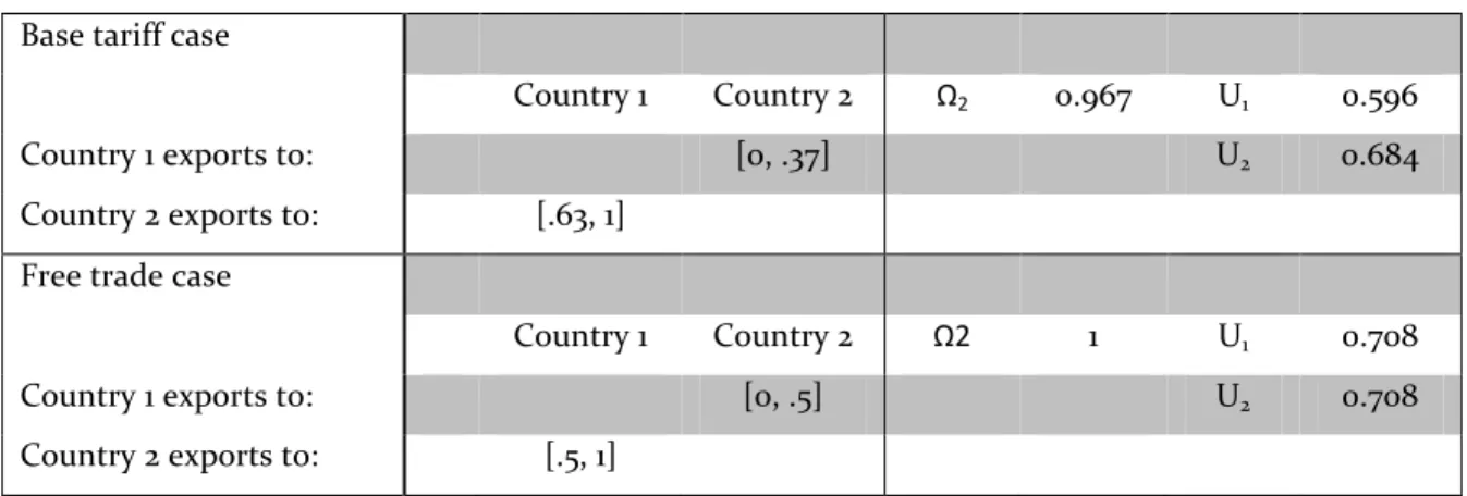
The base tariff case is presented first in the table 3. Each country has at least one
section of the continuum that is non-traded goods. C1 exports between 0 and 0.30 and
imports goods ranging from 0.40 to 1, leaving the range from 0.30 to 0.40 as non-traded
goods for the low-skill country. C2’s non-traded goods range from 0.23 to 0.30 and 0.51 to
0.66. C3’s non-traded goods range from 0.39 to 0.51 and 0.72 to 0.93. C4’s non-traded
goods fall in the range from 0.55 to 0.72. One result of different customs unions is the
changing – increasing, decreasing, or moving – the range on non-traded goods.
38
Following the base tariff case are the simulations for the free trade and two-country
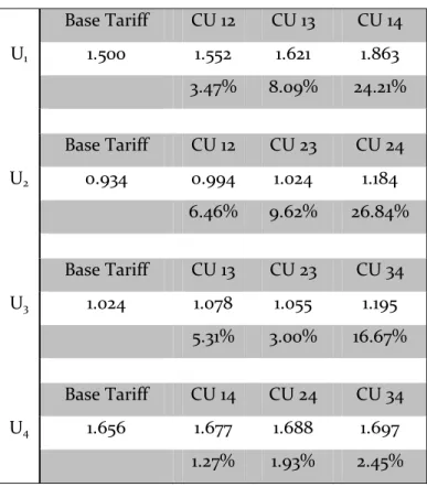
union cases. The changes in utilities are also presented in table 422. There are several
interesting observations. First, C1 strongly prefers a union with C4 – nearly three times more
than a union with C3 and about seven times more than a union with C2. In every case for C1,
a union with partner idrives down the value of Ωi, while driving the value of Ωj up for j≠i.
However, similar to the results in the three-country model where C1 preferred C3 for much
the same reason, C1’s choice of C4 only slightly pushes Ω4 down while Ω2 and Ω3 increase.
As a result of C1 and C4’s union, C4 also no longer exports any goods to C3 as a result of the
changes in the terms of trade. The union of C1 and C4 eliminates both countries ranges of
non-traded goods, as the range of exports and imports both increased. From C1’s
perspective, C4 has replaced C3 as the source for the lower end of the high-skill goods – those
goods ranging from 0.59 to 0.72. Welfare analysis shows that a union between C1 and C4
results in both countries experiencing increases (although C1’s increase is far greater than
C4’s). However, C2 and C3 both experience a decrease in welfare as the terms of trade move
against them.
The results for single partners of C2 are similar to that of C1. C2 prefers C4 as a
partner over C3 and C1. A C2-C4 union provides interesting results, and will continue to do
so when enlargement of the union is examined. Such an agreement eliminates exports (but
not imports) from C3 to C2, as well as exports from C3 to C4. With the partners ‘surrounding’
C3, there is no longer a range of goods for which it is cheaper for either C2 or C4 to import
from C3 rather than either produce for itself or import from its partner. Again, there is a
22