The Mass, Color, and Structural Evolution of Today
’
s Massive Galaxies Since
z
∼
5
Allison R. Hill1, Adam Muzzin2, Marijn Franx1, Bart Clauwens1, Corentin Schreiber1, Danilo Marchesini3, Mauro Stefanon1, Ivo Labbe1, Gabriel Brammer4, Karina Caputi5, Johan Fynbo6, Bo Milvang-Jensen6, Rosalind E. Skelton7,
Pieter van Dokkum8, and Katherine E. Whitaker9,10,11
1
Leiden Observatory, Leiden University, P.O. Box 9513, 2300 RA, Leiden, The Netherlands;[email protected]
2
Department of Physics and Astronomy, York University, 4700 Keele Street, Toronto, Ontario, ON MJ3 1P3, Canada
3
Physics and Astronomy Department, Tufts University, 574 Boston Avenue, Medford, MA, 02155, USA
4Space Telescope Science Institute, 3700 San Martin Drive, Baltimore, MD 21218, USA 5
Kapteyn Astronomical Institute, University of Groningen, P.O. Box 800, 9700 AV Groningen, The Netherlands
6
Dark Cosmology Centre, Niels Bohr Institute, University of Copenhagen, Juliane Maries Vej 30, DK-2100 Copenhagen, Denmark
7
South African Astronomical Observatory, P.O. Box 9, Observatory, Cape Town, 7935, South Africa
8
Astronomy Department, Yale University, New Haven, CT 06511, USA
9
Department of Astronomy, University of Massachusetts, Amherst, MA 01003, USA
10
Department of Physics, University of Connecticut, Storrs, CT 06269, USA
Received 2016 December 23; revised 2017 February 7; accepted 2017 February 19; published 2017 March 15
Abstract
In this paper, we use stacking analysis to trace the mass growth, color evolution, and structural evolution of present-day massive galaxies(log(M* M)=11.5)out toz=5. We utilize the exceptional depth and area of the
latest UltraVISTA data release, combined with the depth and unparalleled seeing of CANDELS to gather a large, mass-selected sample of galaxies in the NIR (rest-frame optical to UV). Progenitors of present-day massive galaxies are identified via an evolving cumulative number density selection, which accounts for the effects of merging to correct for the systematic biases introduced using afixed cumulative number density selection, andfind progenitors grow in stellar mass by»1.5 dexsincez=5. Using stacking, we analyze the structural parameters of the progenitors andfind that most of the stellar mass content in the central regions was in place byz~2, and while galaxies continue to assemble mass at all radii, the outskirts experience the largest fractional increase in stellar mass. However, wefind evidence of significant stellar mass build-up atr<3 kpcbeyondz>4probing an era of significant mass assembly in the interiors of present-day massive galaxies. We also compare mass assembly from progenitors in this study to the EAGLE simulation andfind qualitatively similar assembly withzatr<3 kpc. We identify z~1.5 as a distinct epoch in the evolution of massive galaxies where progenitors transitioned from growing in mass and size primarily through in situ star formation in disks to a period of efficient growth in re consistent with the minor merger scenario.
Key words:galaxies: evolution –galaxies: formation–galaxies: structure
1. Introduction
The mass growth and structural evolution of today’s most massive galaxies is an important tracer of galaxy assembly at early times. These systems are host to the oldest stars, suggesting they were the first galaxies to assemble. Because they are the oldest systems, their progenitors can theoretically be traced to higher redshifts than their low mass counterparts and can be studied from the onset of re-ionization to give a complete history of galactic evolution. Additionally, the most massive systems tend to be the most luminous, and they are the easiest to observe at high redshift with highfidelity. Massive galaxies also provide important constraints on the physics involved in cosmological simulations, as they impose upper limits on growth as well as the efficiency of various feedback mechanisms such as active galactic nuclei, mergers, and supernovae.
Today’s massive (logM* M~11.5) galaxies, to first
order, are a uniform population. They are homogeneous in morphology and star formation, appearing spheroidal, and have low specific star formation rates and high quiescent fractions (e.g., Gallazzi et al. 2005; Thomas et al. 2005, 2010; Kuntschner et al. 2010; Cappellari et al. 2011; Ilbert et al.
2013; Mortlock et al. 2013; Moustakas et al. 2013; Muzzin et al.2013b; Davis et al.2014; McDermid et al.2015; Buitrago
et al.2017). In contrast to today’s massive galaxies, massive galaxies at high redshift show increasing diversity(e.g., Franx et al.2008; van Dokkum et al.2011). With increasing redshift, massive galaxies become increasingly star-forming (e.g., Papovich et al. 2006; Kriek et al. 2008; van Dokkum et al.
2010, 2015; Brammer et al. 2011; Bruce et al. 2012; Ilbert et al. 2013; Muzzin et al. 2013b; Patel et al. 2013; Stefanon et al. 2013; Barro et al. 2014; Duncan et al. 2014; Marchesini et al.2014; Toft et al.2014; Barro et al.2016; Man et al.2016; Tomczak et al.2016), and the massive galaxies that are identified as quiescent at high redshift are structurally distinct from their low-redshift counterparts, as seen in their small effective radii (re) and more centrally concentrated stellar-mass density profiles (Daddi et al. 2005; Trujillo et al. 2006; Toft et al. 2007; Buitrago et al. 2008; Cimatti et al. 2008; van Dokkum et al. 2008; Damjanov et al. 2009; Newman et al.2010,2015; Szomoru et al.2010; Williams et al.
2010; van de Sande et al. 2011; Bruce et al. 2012; Muzzin et al. 2012; Oser et al. 2012; Szomoru et al. 2012, 2013; McLure et al. 2013; van de Sande et al. 2013; Straatman et al.2015; Hill et al.2016).
Although the central regions of massive galaxies contain a higher fraction of the total mass at high redshift, their central stellar densities show remarkably little evolution between z»2 3– and z=0 (e.g., Bezanson et al. 2009; van Dokkum
© 2017. The American Astronomical Society. All rights reserved.
11
et al. 2010,2014; Toft et al.2012; van de Sande et al. 2013; Patel et al. 2013; Belli et al. 2014a; Williams et al. 2014; Whitaker et al.2016)with the majority of stellar-mass build-up occurring in the outer regions (with galaxies growing in an “inside-out”fashion). This mass assembly is thought to occur via minor, dissipation-less mergers; a scenario that is able to account for the size growth, while leaving the interior regions relatively undisturbed (e.g., Bezanson et al. 2009; Naab et al.2009; Hopkins et al.2010; Trujillo et al.2011; Newman et al.2012; Hilz et al.2013; McLure et al.2013; Buitrago et al.
2017). The aims of the present study are to determine whether these trends continue to high redshifts and to identify the epoch when galaxies’central regions assemble their mass.
Obtaining a census of massive galaxies across a broad redshift range is technically challenging, as they have low number densities on the sky(Cole et al.2001; Bell et al.2003; Conselice et al.2005; Marchesini et al.2009; Bezanson et al.
2011; Caputi et al. 2011, 2015; Baldry et al. 2012; Ilbert et al.2013; Muzzin et al.2013b; Duncan et al.2014; Tomczak et al.2014; Stefanon et al.2015; Huertas-Company et al.2016)
and their rest-frame optical emission shifts into the near-infrared(NIR)at intermediate redshifts. To study the evolution of massive galaxies across cosmic time, as a population, necessitates deep and wide NIR surveys to both probe large volumes and obtain rest-frame optical emission to significant signal-to-noise ratios (S/N).
In this study, we use stacking analysis to obtain high-fidelity profiles of the progenitors of massive galaxies out to significant radii (at low z, r>60 kpc). We take advantage of the unparalleled combination of depth and area in the third data release of the UltraVISTA survey (McCracken et al. 2012)to study the structural evolution of massive galaxies out to
z=3.5. Due to incompleteness in UltraVISTA at the highest redshifts considered in this study, we also use the deeper CANDELS F160W data from the 3DHST photometric catalogs (Brammer et al. 2012; Skelton et al. 2014; Momcheva et al. 2016)to extend the redshift coverage to z=5. This is a significant gain in redshift over previous studies, and provides the most extensive redshift range over which the profiles of massive galaxies have been traced.
2. Sample Selection
2.1. Number-density Selection
Linking the progenitors of present-day galaxies to their high redshift counterparts is challenging, as the merger and star formation history (SFH)of any individual galaxy is not well constrained. One way to circumvent these issues is to assume that galaxies maintain rank-order across cosmic time (i.e., the most massive galaxies today will have been the most massive galaxies yesterday, cosmologically speaking). This assumption predicts a constant co-moving number-density with redshift, an outcome used by van Dokkum et al. (2010)to trace the mass and size growth of galaxies from z=2 (corresponding to n =2 ´10-4Mpc dex-3 -1). Subsequent studies have used the same assumptions to select progenitors based on a constant
cumulative number density (e.g., Bezanson et al. 2011; Brammer et al. 2011; Papovich et al. 2011; Fumagalli et al.
2012; Patel et al. 2013; van Dokkum et al.2013; Ownsworth et al. 2014; Morishita et al. 2015), which has the advantage over its non-cumulative counterpart of being single valued in mass.
The selection of progenitors and their descendants at a constant cumulative number density implicitly assumes that mergers and in situ star formation do not broadly affect rank-order, an assumption that has been shown to result in systematically biased progenitor selection (Behroozi et al. 2013; Leja et al. 2013; Torrey et al.2015). To account for the effects of mergers on the progenitor mass, we utilize an evolving cumulative number density selection following the prescription of Behroozi et al. (2013), who use halo-abundance matching within a LCDM
cosmology to connect progenitors and their descendants. It is important to note that we have used the prescription to trace
progenitorsof low-redshift massive galaxies, not thedescendants
of high-redshift massive galaxies, the former of which yield a steeper evolution in cumulative number density due to the shape of the halo mass function, and scatter in mass accretion histories (see Behroozi et al.2013; Leja et al.2013).
2.2. The Implied Stellar Mass Growth of the Progenitors of Massive Galaxies sincez~5
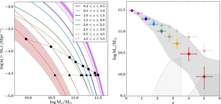
In Figure1we show the integrated Schecterfits of the mass functions of Muzzin et al.(2013b)between0.2< <z 3.0, and Grazian et al. (2015) between 3.5< <z 5.5. These mass functions are based on photometric redshifts determined via ground- and space-based NIR imaging from the UltraVISTA and CANDELS surveys respectively. In the left panel of Figure 1, we show our evolving cumulative number density selection based on the abundance matching of Behroozi et al. (2013). The masses implied from a fixed cumulative number density selection are also shown to illustrate the effect of the bias when the effects of mergers are ignored in the selection. In the right panel of Figure1, the implied progenitor masses from the left panel are plotted for both the fixed and evolving cumulative number density selection, as a function of redshift. The error bars are the uncertainties from the mass functions, which take into account the uncertainties in the photometric redshifts, SFHs, and cosmic variance. The solid gray region represents the scatter in the number densities from the abundance matching of Behroozi et al.(2013), and the hatched regions illustrate an estimate of the mass completeness which is discussed in detail in Section2.3.
Below z=2, Figure 1 shows that both constant and evolving cumulative number density selections yield progeni-tor masses that are consistent within the uncertainties in the mass functions. However, beyondz=2, the bias in thefixed cumulative number density becomes significant, and over-predicts the median progenitor mass. Using the abundance matching technique, we see an overall increase in stellar mass of 1.5 dex since z~5. Our fractional mass growth out to
z=3 is consistent within the uncertainties with Marchesini et al.(2014), who use the same abundance matching selection for ultra-massivelog(M* M)~11.8)descendants, and with
Ownsworth et al. (2014), who use a constant cumulative number density selection that is corrected for major mergers to trace progenitors. Using their correction, they find 75±9% of the descendant mass is assembled after z=3, which is consistent with~80%which wefind in the current study.
incompleteness from UltraVISTA DR1 (the source catalog used in generating the mass functions). However, with the deeper exposures from the third data release (DR3) of UltraVISTA, we are complete to the progenitor masses considered out toz=3.5. To calculate the expected progenitor mass between3.0< <z 3.5, we linearly interpolated the mass between adjacent redshift bins. We also observe a trend of the uncertainties in the mass function monotonically increasing from low to high redshift. Thus, we similarly linearly interpolated the uncertainties to estimate the uncertainty in mass for 3.0< <z 3.5due to uncertainties in photo-z, SFH, and cosmic variance. We also use the uncertainties in the progenitor mass selection as the upper and lower mass bounds for the galaxies that contribute to the resulting stack, thus we select a larger range of masses at higher redshift than at lower redshift.
It has been shown that the Behroozi et al.(2013)prescription for selecting progenitors performs well in terms of recovering the average stellar mass of the progenitors of present-day, high-mass galaxies, however this method fails in capturing the diversity in mass of all progenitors as implied by simulations (e.g., Torrey et al. 2015; Clauwens et al. 2016; Wellons & Torrey 2016), which also predict that the scatter in progenitor masses tends to increase with redshift. Given this large scatter, there is no guarantee that the evolution of other galaxy properties, such as size, will follow from the Behroozi et al. (2013)selection. However, in an upcoming paper(B. Clauwens et al. 2017, in preparation)we will show that, for the property of interest in our study (i.e., the average radial build-up of stellar mass for the progenitors of massive galaxies), the Behroozi et al.(2013)selection yields average agreement with progenitors within the EAGLE simulation.
2.3. Data
2.3.1. UltraVISTA
In order to study the evolution of the average properties of massive galaxies, it was necessary to utilize both wide-field ground-based, and deep space-based imaging for our stacking analysis. Massive galaxies (log(M* M)~11) are
exceed-ingly rare objects, with low number densities (~10-5Mpc-3) on the sky (e.g., Cole et al. 2001; Bell et al. 2003; Baldry et al. 2012; Ilbert et al.2013; Muzzin et al.2013b; Tomczak et al. 2014; Caputi et al. 2015; Stefanon et al. 2015), and require wide-field surveys to characterize a significant popula-tion. To that end, we utilize the NIR imaging from the DR3 of the UltraVISTA survey (McCracken et al. 2012) for our stacking analysis.
The DR3 UltraVISTA catalog (A. Muzzin et al. 2017, in preparation) is a K-selected, multi-band catalog constructed from the UltraVISTA survey. Briefly, the survey covers the COSMOSfield with a total area of1.7 deg2, with deep imaging in theY J H, , , andKsbands. The survey also contains ultra-deep stripes with longer exposures that cover a0.75 deg2area, and also includes imaging in the VISTA NB118 NIR filter (Milvang-Jensen et al. 2013). The newest data release is constructed with the same techniques as the DR1 30-band catalog(Muzzin et al. 2013a), with the inclusion of new and higher-quality data to determine photo-z values and stellar population parameters. The DR3 survey depths in the ultra-deep stripes are ∼1.4 magnitudes deeper than DR1 (with 5s
limiting magnitudes in the ultra-deep regions of 25.7, 25.4, 25.1, and 24.9 inY J H, , andKs).
Several other data sets have also been added since the first data release including 5 CFHTLSfilters,u g r i z* ¢ ¢ ¢ ¢, as well as two new Subaru narrow bands (NB711, NB816). Most
Figure 1.Left: integrated mass functions as a function of stellar mass for differentzranges. Solid and dashed lines indicate the mass functions of Muzzin et al.(2013b) and Grazian et al.(2015), respectively, with color illustrating the redshift. Uncertainties in the mass functions resulting from uncertainties in the photo-zvalues, SFH, and cosmic variance are shown for the highest and lowestz(for clarity). Black circles indicate the cumulative number density selection of Behroozi et al.(2013), with black triangles showing afixed cumulative number density selection for comparative purposes. Right: the mass evolution of the progenitors of alog(M M)=11.5
galaxy atz=0.35. As in the left panel, the circles and triangles show an evolving andfixed cumulative number density selection, respectively. The difference between the circles and the triangles illustrates the bias, especially atz>2, resulting from afixed number density selection. The error bars in they-axis are the uncertainties resulting from the mass function. The error bars in thex-axis represent the redshift range considered. The solid gray regions indicate the1–srange from Behroozi et al.
importantly for this analysis, we also include the latest data from SPLASH (Capak et al. 2012) and SMUVS (PI Caputi; M. Ashby et al. 2017, in preparation). These are post-cryo
Spitzer-IRAC observations that improve the [3.6] and [4.5]
depth from 23.9 to 25.3. Overall this is a 38-band catalog (compared to 30 in Muzzin et al. 2013a), and the substantial increase in depth in theY J H Ks, , , ,[3.6], and[4.5]bands make it a powerful data set for studying massive galaxies at intermediate and high redshifts.
In the right panel of Figure 1, we have indicated our estimated mass completeness limits with the filled hatched regions. To estimate our mass completeness atz<4, we used the limits on the mass functions from Muzzin et al. (2013b)
(which were derived using UltraVISTA DR1), and adjusted the mass limit according to the gain in K-band depth (the K-band limit is 1.5 magntiudes deeper between DR1 and DR3) assuming a constant to-light ratio. Since galaxy mass-to-light ratios decrease with redshift(e.g., van de Sande et al.
2015), this likely represents a conservative estimate of the limiting mass at high redshifts.
2.3.2. Candels
As UltraVISTA DR3 is only mass-complete for our selection out toz=3.5, we use the reddest band available from CANDELS in order to explore redshifts that are unobtainable through UltraVISTA. We select galaxies using the photometric data products from the 3DHST survey(Brammer et al.2012; Skelton et al.2014)from allfive CANDELSfields. As an estimate of our mass completeness in CANDELS, we adopt the limiting mass derived from the 75% magnitude completeness limit (F160W =25.9) in the shallower pointings in the GOODS-S and UDS fields as described in Grazian et al. (2015). They estimated their mass completeness using the technique of Fontana et al. (2004), which assumes the distribution of mass-to-light ratios immediately above the magnitude limit holds at slightly lowerfluxes, and compute the fraction of objects lost due to large mass-to-light ratios. The estimated completeness for CANDELS is indicated in the right panel of Figure1as the gray cross-hatched region.
Although the aforementioned estimates of mass complete-ness take into account galaxies with varied mass-to-light ratios, it is worth stressing inherent uncertainties when determining mass limits at high redshift. Atz>3.5, we increasingly rely on photometric redshifts, as high-fidelity spectroscopic redshifts are fewer in number (Grazian et al. 2015). In addition, submillimeter galaxies (SMGs) likely account for at least a fraction of the progenitors of massive galaxies at high redshift (e.g., Toft et al.2014), and they have been shown to have high optical extinction (e.g., Swinbank et al. 2010; Couto et al. 2016). As the progenitors selected at z>3.5 of this study tend to be less massive than a typical SMG, we do not expect that they will form a significant fraction of the sample. However, we cannot rule out a tail of less, but still obscured sources to lower masses in the distribution of SMGs. This would have the effect of biasing our high-redshift progenitor selection to bluer, less-obscured sources.
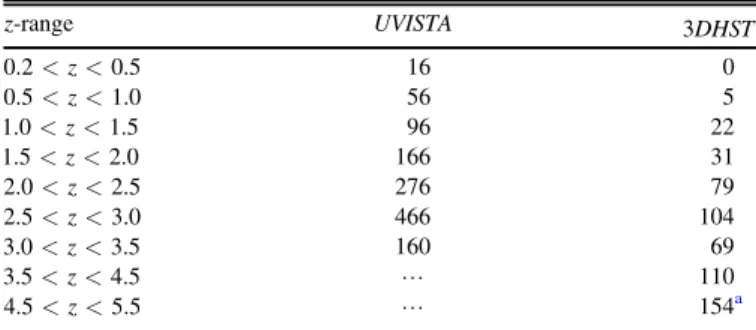
Table1provides a summary of the number of galaxies in the given redshift range, at the implied mass as determined from our evolving cumulative number density selection (see Section 2.1)from both the UltraVISTA and 3DHST catalogs. In order to boost the number of galaxies in UltraVISTA, we have used galaxies from both the deep (DR1) and ultra-deep
(DR3)catalog out to2.0< <z 2.5where we are complete in mass for the shallower catalog (DR1). For the3.0< <z 3.5
bin, we have only utilized the DR3 catalog, as we are incomplete in DR1. As evident from Table1, UltraVISTA has a larger population of massive galaxies at low redshift, while there are 0 galaxies, in all 5 CANDELSfields, that are massive (log(M* M)~11.5) atz=0.35, and only 5 galaxies in the
next highest redshift bin. However, CANDELS is crucial to continue the progenitor selection beyond z>3.5 as we are mass-incomplete in this region with UltraVISTA. Additionally, as galaxies had smaller re at high redshift (see discussion in Section 1 and references therein), the space-based seeing of CANDELS is necessary to properly map the density profiles at these epochs. Thus we utilize both data sets in our analysis.
3. Rest-frame Color Evolution
Cumulative number density selection is a method that selects solely on stellar mass, and is therefore blind to other galaxy properties such as levels of star formation activity. A simple, but effective way to establish star-forming activity in a population of galaxies is to observe where they are located in rest-frameU−VandV−Jcolor space, commonly referred to as aUVJ-diagram. First proposed by Labbé et al.(2005), it is observed that galaxies exhibit a bi-modality in rest-frameUVJ
color space, which is correlated with the level of obscured and unobscured star formation. Actively star-forming and quiescent galaxies separate into a“blue”and“red”sequence in theUVJ -diagram(e.g., Williams et al.2009,2010; Whitaker et al.2011; Fumagalli et al.2014; Yano et al.2016).
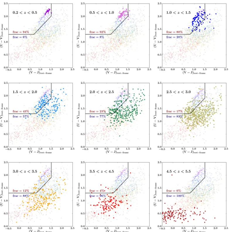
In Figure2, we plot the rest-frameU−VandV−Jcolors for all redshift bins to provide a diagnostic of star formation activity within each stack. Each of the nine panels represents a different redshift range, with galaxy masses selected according to their expected evolving cumulative number density (see Figure1). Thefirst seven panels are galaxies from UltraVISTA DR3, and the last two panels contain galaxies from the 3DHST photometric catalog. It is important to note that we are mass-incomplete for the4.5< <z 5.5bin(see Figure1). However, we have chosen to include it as part of our analysis, with the caveat that we are likely biased toward bluer galaxies. Overlaid in each panel are the color selections used by Muzzin et al. (2013b)to separate quiescent and star-forming sequences.
As one progresses in redshift, it becomes apparent from Figure 2 that the number of galaxies selected dramatically increases. This is a result of three competing effects. Thefirst is
Table 1
Number of Galaxies in Each Redshift Range by Catalog
z-range UVISTA 3DHST
z
0.2< <0.5 16 0
z
0.5< <1.0 56 5
z
1.0< <1.5 96 22
z
1.5< <2.0 166 31
z
2.0< <2.5 276 79
z
2.5< <3.0 466 104
z
3.0< <3.5 160 69
z
3.5< <4.5 L 110
z
4.5< <5.5 L 154a
Note.Above is the number of galaxies found within the mass ranges outlined in Figure1.
a
that the size of our mass range becomes progressively larger with redshift, as seen in the error bars on the right panel of Figure1. By selecting in a wider mass range, we will inevitably select more galaxies. The second effect is that, as the number densities of progenitors increases with redshift, we are progressing toward the lower mass end of the mass functions (Ilbert et al. 2013; Muzzin et al. 2013b; Grazian et al. 2015). Third, at low redshift, the probed co-moving volume is also
smaller than at high redshift. The combined effect is to have our lowest redshift, and least populated stack, contain only 16 galaxies, whereas our most populated stack at 2.5< <z 3.0
contains 276 objects(Table1).
The most prominent trend in Figure 2 comes in the color evolution of the progenitors across redshift. They begin very blue in both U−V and V−J in the lower left of the star-forming sequence and progress red-ward along the star-star-forming
sequence to the upper right until 2.5< <z 3.0, before reddening in V−J and joining the quiescent sequence. Assuming our number density selection is valid, this represents a true evolution inUVJ color.
Figure 3 shows the average UVJ color evolution for each redshift bin, separated into star-forming and quiescent progenitors, and highlights explicitly the trends observed in Figure2. In thisfigure, we see that most of the early (z>3)
color evolution is driven by the star-forming progenitors. At z<3, star-forming progenitors are beginning to quench in large numbers and the two tracks are broadly parallel until z<1 where the quiescent progenitor fractions are high and
UVJ color evolution is driven by the quiescent progenitors. This seems to indicate that massive galaxies begin their existence as star-forming galaxies, which progress along the blue sequence(via aging of the stellar populations, and increase in stellar mass through star formation), before quenching and joining the red sequence.
The progression in theUVJ-diagram between0.2< <z 3.0
is qualitatively similar to Marchesini et al.(2014)who tracked the progenitors of local ultra-massive (log(M* M)~11.8)
galaxies, with the main difference being that this study contains galaxies that are bluer than those of Marchesini et al. (2014). The origin of this difference is rooted in the fact that we select progenitors for a lower local mass galaxy (log(M* M)~ 11.5). Our galaxies in the higher-zbins are also bluer than the sample of Ownsworth et al.(2016), who select progenitors of massive galaxies based onfixed cumulative number density. As previously discussed, a fixed cumulative number density
selection will yield progenitors that are systematically more massive and thus redder inU−V and V−Jcolors, and the inconsistencies in galaxy properties between the samples is likely attributed to differences in stellar mass.
The progression of galaxies between different redshift bins within Figures2and3already provides clues as to the structure of the galaxies within them. Numerous studies find that galaxies in the quiescent region of the UVJ-diagram tend to have highernand smallerre(e.g., Williams et al.2010; Patel et al.2012; Yano et al.2016). However, those analyses are for galaxies at fixed masses and do not connect progenitor to descendant, and therefore do not make a direct evolutionary link. In the next section we examine the size and structural evolution of the galaxies selected using the cumulative number density method.
4. Evolution in Far-infrared Star Formation Rates
In Figures 2 and 3, we see evidence that the evolution of massive galaxies can be broadly separated into two epochs. At z>1.5, galaxies have colors that are consistent with growth mainly through in situ star formation. Atz<1.5, galaxy colors are consistent with quenched systems, with mergers becoming the dominant mechanism for growth. We can estimate this epoch more directly by comparing star formation rates to the mass assembly implied from the evolving cumulative number density selection.
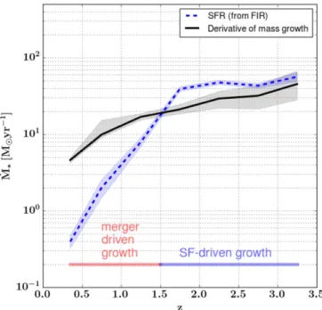
Figure4shows the SFR plotted against the derivative of the progenitor mass growth from the right panel of Figure1. The SFRs are calculated from far-infrared(FIR)luminosities, which are derived from stacks that include Spitzer24μm, and
Herschel PACS and SPIRE bands. For each UltraVISTA stack, FIR stacks were generated in the same manner as described in Schreiber et al.(2015). From Figure 4 of Schreiber
Figure 3. Above is the average rest-frame UVJ color evolution for the progenitors of the quiescent(red symbols)and star-forming (blue symbols) progenitors. The entire sample is plotted in small gray symbols to best illustrate the scatter. The size of the red and blue symbols indicates the quiescent/ star-forming fraction (e.g., a large red circle corresponds to a high quiescent fraction, and a small blue circle corresponds to a low star-forming fraction). The redshift evolution proceeds from bottom left to top right. Purple arrows indicate the direction of quiescence and are labeled for points that bracket a quiescent fraction of 20%. The z=5 point is plotted as an open circle to remind the reader that we are incomplete in that redshift bin, and are likely biased to bluer galaxies.
et al.(2015), we see that we do not have sufficient numbers of galaxies at z>3.5with the CANDELS data to expect a FIR detection. Thus, we only calculate SFRs out to z=3.5. The FIR luminosities were converted to SFRs via the relation from Kennicutt (1998), with a correction factor of 1.6 to convert between the Salpeter IMF used in Kennicutt (1998), to the Chabrier IMF used for the DR3 catalog.
In order to more directly compare the net stellar mass growth as implied from the abundance matching technique to the stellar mass growth from star formation, a 50% conversion factor has been applied to the SFR to account for stellar mass which is lost in outflows from stellar winds(see van Dokkum et al. 2008, 2010). From Figure 4, we see that SF is able to account for all of the stellar mass growth atz>1.5, with little to no contribution from mergers. In contrast, the SFR at z<1.5are insufficient to explain the mass growth, suggesting stellar mass is accreted via mergers.
Between1.5< <z 2.5, the stellar mass growth predicted from star formation is greater than what is found from the abundance matching techniques by 0.1 0.2 dex– . This discre-pancy is also seen in model and observation comparisons(see Madau & Dickinson 2014; Somerville & Davé 2015), with potential for the FIR SFRs to be over estimated during this epoch (see Madau & Dickinson2014and discussion therein). In spite of this, the FIR SFRs support the notion that massive galaxies grow via star formation until z~1.5, where merger driven growth dominates, consistent with the rest-frame UVJ
colors, and what is found in the literature (see Section1 and references therein).
5. Analysis
5.1. Stacked Images
For galaxies at z<3.5, images were stacked using
48 ´48cutouts taken from the UltraVISTA mosaics, which contain both deep and ultra-deep stripes. For each cutout, SEDs were generated using the ancillary data available in the UltraVISTA and CANDELS source catalogs. These SEDs were used toflag potential active galactic nuclei(AGN), which were removed from the resultant stack. The individual cutouts were also visually inspected to remove objects that were identified as doubles or triples (i.e., were not separated by SExtractor; Bertin & Arnouts 1996), or in close proximity to saturated stars to maintain imagefidelity. In total,<4%of the entire sample was discarded.
Cutouts were centered using coordinates taken from the UltraVISTA DR1(only deep stripes)and DR3(only ultra-deep stripes)catalogs, with cubic spline interpolation performed for sub-pixel shifting. For galaxies atz>3.5, images were stacked using24 ´24cutouts, taken from thefive CANDELSfields (AEGIS, COSMOS, GOODS-S, GOODS-N and the UDS), with images centered using the coordinates from the 3DHST photometric catalogs(Brammer et al.2012; Skelton et al.2014)
with sub-pixel shifting also performed using cubic spline interpolation.
From these cutouts, bad-pixel masks were also constructed using SExtractor segmentation maps. These bad-pixel masks were also used to construct a weight map for thefinal stack by summing the bad-pixel masks (in a similar manner to van Dokkum et al.2010).
For the UltraVISTA stacks, the ultra-deep and deep cutouts were weighted differently in the final stack as the ultra-deep
stripes have an exposure time of a factor~10 greater than the deep stripes. The images are weighted by the expected S/N gain, based on the exposure time(i.e., an image with a factor of
∼10 more exposure time will result in a S/N gain of∼3). The exact exposures varied between theY,J,H, andKsbands, with the relative weights between the deep and ultra-deep also changing slightly.
The cutouts were normalized to the sum of theflux contained in the central1. 5 ´ 1. 5(corresponding to10´10 pixelfor UltraVISTA images and 25´25 pixel for CANDELS images). A weighted sum was performed on the masked cutouts, with the cutouts contained in the ultra-deep stripes given a heavier weight than those in the deep stripes. This summed image was divided by the weight map to provide the
final stack.
For the UltraVISTA stacks, PSFs were generated similarly to the stacked-galaxy images. Stars within a magnitude range were chosen such that the stars had sufficiently high S/N without being saturated(»16.5Ks-band magnitude). The stars were treated in the same manner as the stacks of the galaxies (i.e., normalized and averaged). To account for variations in the PSF across the mosaic, 12 different PSFs for each band were generated corresponding to 12 different regions of the mosaic ultra-deep stripes, and 9 for the deep stripes. Afinal PSF for the relevant band was generated from a weighted average of the 12/9 PSFs, with the weights corresponding to the number of galaxies from eachfield that went into the making of the stack. Thus, each stack has a uniquely generated PSF.
For the CANDELS F160W stacks, PSFs for each of thefive
fields were taken from the 3DHST-CANDELS data release (Grogin et al. 2011; Koekemoer et al. 2011; Skelton et al. 2014). In a similar manner to the UltraVISTA stacks, the PSF for the relevant band was generated from a weighted average of the PSF from each field, with the weights corresponding to the number of galaxies from eachfield that contributed to thefinal stack; thus each F160W stack similarly has a uniquely generated PSF.
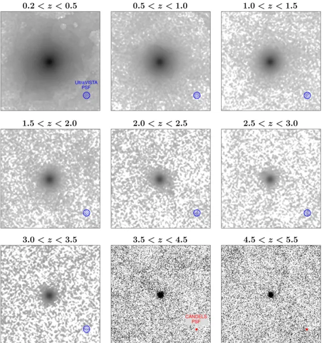
Figure5displays the results from the stacking analysis. Each panel contains a 24´24 display of one of the UltraVISTA bands(eitherY,J,H, orKs), except the last two panels which are stacks of the CANDELS F160W data. The UltraVISTA stacks are all displayed at the same color scale to highlight the differences in background, which increases with increasing z. The F160W stacks were plotted at a different color scale for clarity, as the background is much higher.
In addition to the stacks in Figure 5, 100 bootstrapped images were also generated for each stack to constrain uncertainties in the structural parameters determination (see Section5.2). Each bootstrapped image also comes with its own unique PSF that reflects the proportion of galaxies from various
fields in the same manner as the original stacked images.
5.2. Sérsic Profile Fitting
Sérsicfitting (Sérsic 1968)of the stacked and bootstrapped images was performed using GALFIT(Peng et al.2010), with the only constraints imposed on the fits being to restrict the value of the Sérsic indices to between1 <n <6. Figure 6
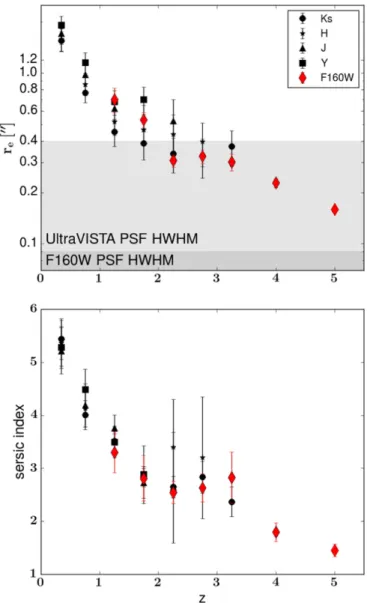
symbol plotted unfilled to mark where we are incomplete. The HWHM of the UltraVISTA and CANDELS PSFs are indicated on the top panel in light gray and dark gray regions respectively. As seen from the top panel of Figure 6, we resolve the stacked images to within an effective radius for UltraVISTA below z=2, and the re is fully resolved for CANDELS in all redshift bins. Additionally, for the redshift bins for which we have stacks for CANDELS and UltraVISTA, the derived sizes and Sérsic indices are roughly consistent with one another, suggesting our ground-based structural parameters are reliable.
Absent from Figure 6are best-fit values forreandn below
z=1 for the F160W band. In these redshift bins, at the mass ranges considered, there were no galaxies present in the catalog
to contribute to a stack(see Table1). Similarly, best-fit values for the UltraVISTA bands are not present for all redshift bins with theY,J,H, andKsdropping out atz=2, 2.5, 3, and 3.5 respectively, due to insufficient signal-to-noise in the resultant stack (and the fact that we are incomplete in UltraVISTA atz>3.5).
5.3. Evolution in re
Due to the progression of redshift between the stacks, there andnare measured at varying rest-frame wavelengths. In order to measure as closely as possible the same rest-frame wavelength, we have measured how re and n change with wavelength. In the left panel of Figure7we have plottedreas a
Figure 5.Sample stacked images for each redshift bin. Thefirst seven panels contain stacks from the UltraVISTA data, with each panel containing a stack from the band that is closest to the rest frame 0.5μm. TheY-band is chosen for stacks atz<1, theJ-band at stacks1< <z 2, the H-band at2< <z 3, theKs-band at
z
3.0< <3.5. The UltraVISTA stacks are all displayed at the same color scale to highlight differences in background and S/N. The last two panels areF160W stacks, and are plotted at the same scale to each other, although different from the UltraVISTA images for clarity, as the background is much higher in the higher-z
function of rest-frame wavelength. Different colors correspond to different redshift bins, and different symbols demarcate the observed band (with the same symbol convention as in Figure 6). The desired rest-frame wavelength of 0.5μm was chosen to minimize extrapolation and still be red-ward of the optical break.
Atz<3, we have measurements in multiple bands andfind that the effective radii decrease with increasing rest-frame wavelength, which is consistent with results from previous studies (e.g., Cassata et al. 2011; Kelvin et al.2012; van der Wel et al. 2014; Lange et al. 2015). However, between
z
2< <3, the uncertainties are consistent with little to no evolution inrewith rest-frame wavelength. When considering the evolving properties of the progenitors with redshift, this result is also consistent with the literature. van der Wel et al. (2014), who measured the sizes of galaxies from CANDELS at
z
0< <3, found the size gradient with rest-frame wavelength
was steepest for galaxies at high mass and low redshift, and
flatter for low-mass galaxies. As the progenitors decrease in mass with redshift, we expect aflattening of this gradient. The difference in size gradients is also seen in local populations. Kelvin et al.(2012)found size gradients to be flatter for late-type galaxies in the GAMA survey. Because we only have measurements in one band forz>3.5and we are dominated by late-type galaxies at high redshift, we have not extrapolated
re between 3.5< <z 5.5 and assume the measurement is representative of thereat 0.5μm. This is assuming that the size gradient will be flat for low-mass, late-type galaxies at high redshift.
In the right panel of Figure7, we have plottedreat 0.5μm as a function of redshift. It is clear from both panels of Figure7
that the re decreases out to z=5, which is consistent with previous results using a diverse set of methods to select progenitors (e.g., van Dokkum et al. 2010; Williams et al.
2010; Damjanov et al. 2011; Mosleh et al. 2011; Oser et al. 2012; Barro et al. 2013; Patel et al. 2013; Straatman et al.2015; Ownsworth et al. 2016). In spite of the different choice of progenitor selection, belowz=2 our measurements fall broadly on the same relation found by van Dokkum et al. (2010) (our values are systematically larger, but this is likely a reflection of our slightly higher mass selection). This result is not surprising, and the consistency is reflected in the right panel of Figure1, where atz<2, the mass of the progenitors chosen using afixed versus evolving cumulative number density are within the uncertainties in both the mass function and the semi-analytic models. Although we measure a slightly steeper relation than van Dokkum et al. (2010), it is surprising how well the relation is extrapolated at z>2 given that we are selecting galaxies that are distinct in mass from the fixed cumulative number density selection.
In Figure 8, we investigate the evolution of the mass–size plane. We have taken the values ofrefrom the right panel of Figure7, and plotted them against their respective progenitor masses, with the highest mass associated with the lowest redshift bin. For comparison purposes, we have over-plotted the mass–size relations from Shen et al.(2003)and Lange et al. (2015)for both early- and late-type galaxies. For Lange et al. (2015), who investigate the mass–size relations as a function of rest-frame wavelength, we use their g-band relations which correspond most closely to a rest-frame wavelength of0.5 mm . The measuredrefrom our stacking analysis fall on the SDSS and GAMA mass–size relations for early-type galaxies at z<0.1. However, for all other redshift bins our galaxies fall below the local mass–size relation, consistent with van Dokkum et al. (2010). Also plotted in Figure 8 are simple single (dashed–dotted line)and double (solid line)power-law
fits of the form
re=aM*b ( )1
r M M
M
1 2
e
0
* *
g
= a⎛ + a b
-⎝
⎜ ⎞
⎠
⎟ ( )
From Figure8, we see that the double power law is a more appropriate fit for our data, with the parameters g=2.9´ 10-4, a=0.35, b=2.1´103, and log M M 14.77
0 =
( ) .
Continuing with the plotting convention of previousfigures, our z
4.5< <5.5point has been plotted as an open-face symbol to highlight incompleteness issues within that bin. It is interesting to note that this point has not been included in any of the
Figure 6.Top: best-fit effective radius in units of arc seconds as a function ofz
power-lawfits, and the fact that it falls on the extrapolation of the double power law is not designed.
The evolution in the mass–size relation in Figure8 can be broadly separated into two phases. At z>1.5, the mass–size evolution is relatively linear (in log-log space), with most points falling along a single power law. At z<1.5, the size growth becomes more efficient, and no longer follows the same single power law as before. This is broadly consistent with patterns we have seen in Figures 3 and 7, i.e., that star formation and mergers are dominating mass and size growth at different epochs, with this changeover occurring at z~1 2– . Before this time, mass was primarily added via star formation, which has been shown to be ineffective at altering the structure of massive galaxies (Ownsworth et al. 2012). At these redshifts, we see a marked increase in the quiescent fraction of the progenitors. As star formation is no longer an available pathway to mass growth, the growth is dominated by minor mergers, which efficiently increases the re(see Section1 and references therein).
5.4. Evolution in n
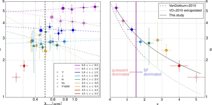
Figure9is analogous to Figure7, except we investigate how the Sérsic indexnchanges with rest-frame wavelength in place of re. From the left panel of Figure 9 we see little to no evolution in n with wavelength at any redshift. We have therefore taken an average n weighted by the bootstrapped uncertainty in each band to measure a representativenfor each redshift bin. Atz>3, where we only have one measurement for each stack, the measurement was considered representative. The resulting values are plotted in the right panel of Figure9. Figure9 shows a clear downward trend of n with redshift, consistent with previous findings out to z=2 (e.g., van Dokkum et al. 2010). This trend is also expected given the
Figure 7.Left: the effective radius plotted against the rest-frame wavelength for the stacks in all bands measured. Different shaped symbols correspond to the observed band with the same symbol convention as Figure6. Each color corresponds to a different redshift range, with the color convention the same as Figure1, including plotting the4.5< <z 5.5symbol as open-faced to remind the reader that we are mass-incomplete for thatzbin. Dashed colored lines are linear bestfits to the data, with the bold, black, vertical dashed line marking the rest-frame 0.5μm point, which the data atz<3are extrapolated/interpolated to, to compare the same rest-frame sizes.zranges with only one measurement are not extrapolated for reasons discussed in Section5.3. Right: the size evolution of the progenitors of massive galaxies sincez~5. Colored circles are the extrapolated/interpolated point atz<3, or the“raw”measurements atz>3. Over-plotted are the size–zrelation of van Dokkum et al.(2010)and the size relation derived for this study.
Figure 8. The implied mass–size evolution of the progenitors of massive galaxies. Circles are measurements from the stacks from the present study, with each point representing a different redshift. Thereplotted above are the same
evolution in the quiescent fraction. Actively star-forming galaxies tend to have lowernor be more centrally concentrated than their quiescent counterparts (e.g., Freeman 1970; Lee et al. 2013; Lange et al.2015; Mortlock et al. 2015); thus at z>1 the decrease in n is likely driven by morphological changes between each redshift bin, which we also see reflected in the evolution of the mass–size relations (Figure 8). van Dokkum et al. (2010) also found n to decrease with redshift, although their relation is steeper than the one measured in the current study. However, the n–z relation from van Dokkum et al. (2010) was derived from galaxies at z<2, where the slopes are comparable, but where we measure systematically highern.
5.5. Mass Assembly
Equipped with measurements ofreandn, we can investigate surface-density profiles, and mass assembly as a function of radius. To generate these profiles, we have assumed that the mass-to-light ratio is constant across the profile, and that all the mass can be found within a radius of 75 kpc. Given these assumptions and that the integrated mass within 75 kpc must equal the total mass found in the right panel of Figure 1(i.e., the same constraints used in van Dokkum et al.2010), we have generated stellar-mass density profiles, which can be found in Figure10.
Figure10shows the Sérsicfits using the values ofreand n for each redshift bin in the right panels of Figures 7 and 9
respectively. The transition between the solid and dashed lines for each profile marks the point when the error in the background becomes significant. Since many of the values of
reand n are either interpolated, or averaged(see Sections5.3 and 5.4), the profiles from which this transition point was determined were the closest to the rest-frame wavelength of
0.5μm (these are the same bands that are displayed in Figure5).
Figure 10 illustrates that the majority of mass build-up in galaxies since z=4 occurs in the outskirts, consistent with previous findings and the inside-out growth paradigm for massive galaxies (van Dokkum et al. 2010; Toft et al. 2012; Bezanson et al. 2013; van de Sande et al. 2013; Belli et al. 2014a; Margalef-Bentabol et al. 2016; Buitrago et al.
2017; Jung et al.2017). It is only atz=5 that we begin to see significant growth in the inner regions. Important to note is that as we are incomplete in that redshift bin, we will be biased toward blue, and possibly diskier galaxies which would likely have lower values of n. However given the trend of Sérsic index with redshift found in Figure9, this does not seem to be an unreasonable depiction of the progenitors.
In Figure 11, we have divided the surface mass density profile for each redshift bin from Figure10by the surface mass density profile at 0.2< <z 0.5. In this way, we are able to trace the fractional mass assembly as a function of radius. At the highest redshift bins we see the central regions are thefirst to form, with very little of the stellar mass beyond3 kpc in place atz~5. Between 3.0< <z 4.5 we see rapid growth, with the fraction of mass assembled in the inner regions more than doubling. It is also in this redshift interval that a not insignificant fraction of stellar mass is assembled between 3 and10 kpc. We can trace the redshift of formation as a function of radius by tracing the horizontal dashed line in Figure 11, which marks the point at which half of the stellar mass was assembled. As one traces from small to large radii, the dashed line crosses different colored regions, indicating that the interior regions were the first to assemble, with the outer regions assembling at later and later times, indicative of “inside-out”growth.
We can trace this growth quantitatively by considering the total mass in and outside of the3 kpcboundary. We have
de-Figure 9.The same as Figure7, but with Sérsic index instead of the effective radius. Left: Sérsic index plotted against the rest-frame wavelength with the same plotting convention as Figure7. As the relation betweennandlrestis consistent withflat, there is no extrapolation to the 0.5μm point. Instead, the values are averaged
to produce a representativenfor eachzbin. Right: the evolution ofnwithz. Over-plotted are the best-fit relation for this study and the relation from van Dokkum
projected the surface density profiles of Figure 10, and separated the mass growth into stellar mass assembly that is within r<3 kpc, and exterior to r>3 kpc. The total mass
assembly is indicated in black, and is the same mass assembly seen in the right panel of Figure1. From the red line, we see continuous, albeit decelerating, mass assembly from z=5 to
z=0. This is inconsistent with previous works, such as van Dokkum et al. (2010)and Patel et al. (2013), who found the interior regions are consistent with no assembly sincez=2, oft cited to be evidence of “inside-out” growth, although it depends on precisely what is meant by this term.
It is important to note from Figures 11 and 12 that even though the regions outside3 kpc experience a greater growth rate than the inner regions, there is still significant mass build-up fromz=5 to z=0 in the interior. Although the growth between the inner and outer regions is not self-similar, the growth is not necessarily“inside-out”as described in previous works(e.g., van Dokkum et al.2010; van de Sande et al.2013), especially when considering the mass assembly at z>3. At these redshifts, significant stellar mass is assembled at all radii (although mass accretion is concentrated in the central regions).
5.6. Comparisons with Simulations
There have been many comparisons between the mass growth of galaxies in extra-galactic surveys(i.e., mass functions) to hydrodynamical galaxy simulations (e.g., Vogelsberger et al.2014; Schaye et al.2015). In fact, the EAGLE simulation has been calibrated to reproduce the galaxy stellar mass function at z=0. However, there remain few examples (e.g., Snyder et al.2015; Wellons et al.2015; Tacchella et al.2016b)in the literature that explicitly compare the evolution of structure in simulations to observations. In this section, we endeavour to make such a comparison.
In Figure13, we see how the mass assembly as implied by our observations compares to the EAGLE simulation (Schaye et al. 2015). In Figure 13, we see the total mass assembly
Figure 10.Top: the projected surface mass density profiles for our stacks(presented in both log-linear and log-log scales). Each profile is a Sérsic, with thereandn
taken from the right panels of Figures7and9, with the constraint on normalization that the integrated mass within75 kpcbe equal to the implied progenitor mass from Figure1. The fadedfilled region corresponds to profiles within the 16th and 84th percentile from the bootstrapped images. The transition from a solid to dashed line in the profile marks the point where the error in the profile is at the level of the background. The PSF HWHM for each redshift is also marked with a vertical line ending in a star at the top of each plot. Bottom: the fraction of assembled mass with radius for each profile(presented in both log-linear and log-log scales). The curves are all normalized to the total mass at0.2< <z 0.5. The curve for4.5< <z 5.5is faded to remind the reader that we are mass-incomplete in thatz-bin.
(black line), the mass assembly within a3 kpcaperture and the mass assembly outside a 3 kpc aperture. Also plotted in Figure13are the de-projected aperture masses from this study
for comparison. The progenitors in EAGLE are defined as the “true”progenitors, and are selected in a similar method to the dark-matter halo merger trees from Behroozi et al. (2013), which inform the abundance matching technique; i.e., only the most massive progenitor from the precursors of a merger is considered. The progenitors were traced from all galaxies within the EAGLE simulation that have a stellar mass within
0.1 dex of log(M* M)~11.5 (i.e., chosen to match the
starting point of this study), which amounted to 24 galaxies. The aperture masses from EAGLE quoted above are averages from the progenitors of these 24 galaxies.
A qualitative comparison between the simulations and the observations show remarkable agreement. For the mass within
3 kpc, the agreement is always within a factor of 2, which is within the uncertainty associated with the assumptions made when determining stellar masses from photometry (Conroy et al.2009). Both methods predict the same overall trend, i.e., that there is a steady build-up of stellar mass within3 kpc, and rapid assembly at later times at radii larger than 3 kpc. The main difference between the simulations and observations is that EAGLE predicts a more rapid assembly of the progenitors. The progenitors in EAGLE must assemble more mass in the same period of time in order to achieve afinal stellar mass of
M M
log * =11.5 at z~0.3. This offset is not entirely
unexpected, given differences between the evolution of the observed and simulated galaxy stellar mass functions at highz
in the mass ranges considered for this study(~1010 1011M
– ,
Furlong et al.2015).
The progenitors in EAGLE must assemble more mass in the same period of time in order to come to the same descendant mass byz~0.3;and given the agreement with observations at r<3 kpc, nearly all of this mass growth must occur in the outer regions. This suggests the progenitors in EAGLE are more centrally concentrated than observed, except at z>4. Between4 < <z 5, the fraction of stellar mass outside a3 kpc
aperture is in broad agreement with the observations, which do not follow the trend atz<4. One possible reason for this is that the effective radius at these redshifts is close to1 kpc, which suggests nearly all of the total bound mass in the galaxy would be within3 kpc, which is not true at lower redshifts.
Some caveats that could affect the above comparison are some assumptions that were made in the observations, in particular the assumption of a constant mass-to-light ratio for our surface mass density profiles. If there is a strong gradient of stellar age with radius in the progenitors, and the interiors are older (which would be consistent with what we see in Figure 11), then we would over-predict the fraction of the total stellar mass that is located at large radii, bringing us closer to agreement with the simulations. A similar effect would be expected if there are also strong gradients in dust. An analysis of forthcoming virtual observations from EAGLE with the effects of dust and inter-cluster light taken into account would be a better comparison, the investigation of which is beyond the scope of this paper.
6. Discussions and Conclusions
6.1. Mass and Size Growth atz<2
In this paper, we have selected the progenitors of today’s massive galaxies through an evolving cumulative number density technique, and have made image stacks to infer their evolution with redshift. Based on rest-frameU−VandV−J
Figure 12.The total projected mass within3 kpc(red line)and outside3 kpcas implied by integrating the profiles from Figure10. The last symbol is plotted as open faced to remind the reader that we are mass-incomplete in thatzbin. There is growth in both radial regions, however the growth is not self-similar with the growth outsider=3 kpcproceeding at a faster pace than the inner regions.
colors, wefind that the progenitors of massive galaxies become increasingly star-forming out to higher redshifts, and by assuming Sérsic profiles for the mass distribution wefind the progenitors decrease in both re and n. These trends are qualitatively similar to previous studies which select based on
fixed (e.g., van Dokkum et al. 2010; Patel et al. 2013; Ownsworth et al.2014)and evolving(Marchesini et al.2014)
cumulative number densities at z2
Although the qualitative trends are consistent with the literature, there are quantitative differences, especially in regards to the evolution of the central mass densities with redshift. Previous works(e.g., van Dokkum et al.2010,2014; Patel et al.2013)have found little to no mass assembly in the inner regions(r<2 kpc)and that mass assembly occurs in an inside-out fashion, with the majority of mass growth since z~2 occurring atr>2 kpc (although in van Dokkum et al.
2010 at~1 kpc, there is a spread in mass density of at least
0.1 dex since z=2, suggesting modest mass growth). In this study, we find the central regions have accumulated»50% of their mass between2.0< <z 2.5, but continue to experience mass growth out toz=0.2, albeit at a lower rate(i.e., wefind that~90%of the mass within2 kpcwas in place byz~1).
The suspected cause of this discrepancy is the differences that arise between afixed versus evolving cumulative number density selection. By using afixed cumulative number density selection, one is biased toward the most massive progenitors (e.g., Clauwens et al.2016; Wellons & Torrey2016). This is a result of the fact that an abundance matching technique (i.e., Behroozi et al. 2013) predicts higher number densities with increasing redshift, whereas afixed cumulative number density will select galaxies at a steeper point in the mass function which is inhabited by higher mass galaxies. We have tested this hypothesis by re-measuring the surface mass density profiles for a fixed cumulative number density selection(see Figure1
for the mass assembly history), and do find that the redshift evolution in central regions of the stellar surface mass density
profiles is considerably weaker than for an evolving number density selection (Figure14). Details of this analysis can be found in theAppendix.
In contrast to afixed cumulative number density selection, van Dokkum et al. (2014) selected galaxies based on their stellar surface mass density within1 kpc(i.e., “dense cores”), and found evidence that the interiors are formedfirst, with the outer radii forming around them. This inconsistency can also be attributed to selection, and the progenitors van Dokkum et al. (2014)select are likely a subpopulation of the progenitors of massive galaxies. Since they are selected on central stellar density, and central stellar density is correlated with quies-cence, they will not select star-forming progenitors. This is evidenced by the differences in quiescent fraction at
z
2.0< <2.5; van Dokkum et al. (2014) find a quiescent fraction of 57%, whereas the selection of the current study has a quiescent fraction of 23% in the same redshift range.
The most massive progenitors are likely to host older stellar populations, have less star formation, and have more compact configurations due to rapid early assembly. As these progenitors would have assembled first, they experience more passive evolution in their central regions betweenz=2 and today(e.g., van de Sande et al. 2013). The star-forming progenitors, however, must still quench, and might involve more violent events, such as disk instabilities which result in compaction, i.e., the driving of mass toward smaller radii(Barro et al.2014; Dekel & Burkert 2014; Tachella et al. 2016a, 2016b). By averaging these populations, one would expect modest gains in stellar mass density in the central regions, which is what is seen in our analysis.
An important caveat to consider when selecting progenitors at systematically higher number densities is the effect of a lower normalization to the mass profiles. Our profiles are designed such that 100% of the stellar mass, as determined from the mass functions as outlined in Figure 1, is contained within75 kpc. If at eachzstep we have a slightly lower mass
selection than studies based on a fixed cumulative number density selection, the normalization of the profile will tend to lower values, which imposes sustained mass growth in the central regions(see Figure14, and discussion in theAppendix). Although wefind the progenitors continue to assemble mass at all radii, the growth rate at small and large radii is not self-similar. The fractional growth rate is higher at larger radii, consistent with the idea that minor mergers play a dominant role in the mass assembly atz<1.5, and especially atz<1as found by Newman et al.(2012), Whitaker et al.(2012), Belli et al.(2014b,2015), and Vulcani et al.(2016).
This is also in agreement with our quiescent fractions, which are>90% at z<1, suggesting that the majority of the mass growth cannot be from star formation. However between
z
1< <2 our star-forming fraction exceeds 50%, suggesting the increasing importance of star formation in mass assembly, which is in broad agreement with Vulcani et al. (2016) who
find that star formation and minor mergers play equal roles in mass growth during this epoch. Additionally, Hα maps of massive star-forming galaxies between 0.7< <z 1.5 reveal that the disk scale lengths are larger in Hα than in the stellar continuum, suggesting that star formation also contributes to the mass build-up at large radii (Nelson et al. 2016), and not just in the inner regions.
6.2. Mass and Size Growth atz>2
In addition to comparisons with other works, which are largely limited to z<2, we have selected progenitors and generated stacks for galaxies out toz=5.5. In this regime we see a continuation of the trends at z<2, i.e., progenitors are smaller and have Sérsic indices that imply more disk-like configurations than spheroidal. This is consistent with the evolution of our quiescent fraction, which continues to decrease with increasing z, suggesting the progenitors are dominated by star-forming galaxies which also tend to have disk-like morphology, which is observed in massive galaxies at high redshift(e.g., van der Wel et al.2011; Wuyts et al.2011; Bruce et al.2012; Newman et al.2015). This is in agreement with the prediction of Patel et al.(2013), who posited that the progenitors of massive galaxies atz>3will continue the trend toward smaller sizes.
The trends in the evolution of the mass–size relation,re, the Sérsic index, the UVJ color evolution, and the FIR derived SFRs all corroborate the idea that z~1.5 represents a transitional period in how the progenitors of massive galaxies assemble their mass. Atz>1.5, the UVJ colors and the FIR SFRs suggest the progenitors are actively forming stars, and the Sérsic index suggests those stars are consistent with being distributed in an exponential disk. The change in power-law slope at z~1.5 in the evolution of the mass–size plane suggests a change in assembly method; one in which the size evolves more efficiently with mass than at higher redshifts, consistent with the minor merger scenario (see Section1 and references therein). This is further corroborated by the fact that the FIR SFR is insufficient to account for the rate of stellar mass assembly at z<1.5(Figure4).
This study supports the scenario that the progenitors of massive galaxies begin with a disk-like morphology, with the disk forming concurrently with the central regions (i.e., the “bulge”). At some point, the disk morphology is destroyed, either by major mergers, or disk instabilities which may also be responsible for the increase in quiescent fraction. Evidence of
disks(e.g., van Dokkum et al.2008; van der Wel et al.2011; Wuyts et al. 2011; Bruce et al. 2012; Bell et al. 2012) and rotation (Newman et al. 2015) in massive compact quenched galaxies are seen at intermediate(1.5< <z 3)redshifts, which confirms that at least some of the massive progenitors host/ hosted a disk-like morphology. By z=1.5, assembly is less violent, with mass growth dominated by minor mergers, and more passive quenching(i.e., gas exhaustion)untilz=0.
The scenario that the progenitors of massive galaxies begin as disks has support in cosmological simulations. Fiacconi et al.(2016b)simulated the assembly of the main progenitor of az=0 ultra-massive elliptical, and found the progenitor to be disk-dominated, with an exponential brightness profile atz>6
that had experienced several major mergers at z>9. The “survival”, or more accurately, the reassembly of the disk after a major merger is feasible, provided the major mergers are sufficiently gas rich(e.g., Hopkins et al.2009). Fiacconi et al. (2016b) also calculated the Toomre parameter for their simulated disk and found it to be stable against fragmentation for all resolved spatial scales, with the disk supported by a turbulent interstellar medium thought to be due to feedback from star formation. They also predict that gas-rich star-forming disks atz>5should not host a significant bulge, but rather be built up by mergers occurring at2 < <z 4(Fiacconi et al.2016a). This is consistent with our analysis, which shows the majority of the stellar mass in the central regions (i.e., r<1 kpc, which we take as a proxy for the bulge) is assembled between2.0< <z 5.5.
Stacking analysis is a useful tool to probe the average properties of low surface brightness features of a population of galaxies. However, specific aspects of the morphology are lost in a stack. To verify our hypothesis about the nature of the progenitors of today’s massive galaxies will require resolution and sensitivity of space-based observatories such asHST. At highz, the rest-frame optical emission is shifted further into the infrared, which future space observatories such as JWSTwill observe at wavelengths beyond the K-band, will prove to be invaluable in determining the nature of“regular”galaxies atz>2.
7. Summary
To briefly summarize the paper, we have traced the stellar mass evolution of the median progenitors of logM* M= 11.5 galaxies at z=0.35 using abundance matching techni-ques. Using photometric data from the UltraVISTA and 3DHST surveys and their associated catalogs, we have used stacking analysis to trace the mass assembly of the progenitors out toz=5.5. Byfitting the image stacks with 2D convolved Sérsic profiles, we have found the following.
1. Selecting progenitors based on an evolving cumulative number density selection results in progenitors that are less massive than if selected based on afixed cumulative number density selection. This discrepancy becomes significant atz>2.
2. The progenitors of massive galaxies become progres-sively more star-forming, with star-forming fractions exceeding 50% at z>1.5 as determined by their rest-frameU−Vand V−Jcolors.