ISSN: 2252-8938, DOI: 10.11591/ijai.v6.i1.pp8-17 8
CBIR of Brain MR Images Using Histogram of Fuzzy Oriented
Gradients and Fuzzy Local Binary Patterns
Athira TR, Abraham VargheseDepartment of Computer Engineering, Adi Shankara Institute of Engineering and Technology, Kalady, India
Article Info ABSTRACT
Article history: Received Nov 3, 2016 Revised Jan 7, 2017 Accepted Feb 16, 2017
Retrieval of similar images from large dataset of brain images across patients would help the experts in the decision diagnosis process of diseases. Generally used feature extraction methods are color, texture and shape. In medical images texture and shape features are most efficient. Histogram of Oriented Gradients (HOG) and Local Binary Pattern (LBP) are good descriptor for brain MR image retrieval. But there are many challenges facing in medical application. An empirical study of the impact of increasing bins number in the HOG descriptor concluded that larger the number is more accurate the descriptor is. In fact this is due to the reduction of orientations range that each bin covers. Despite the efficiency of augmenting the bins number, this technique has limited spatial support as the augmentation of the number of bins used leads to increase the histogram dimension. So here proposed a method called Histogram of Fuzzy Oriented Gradients (HFOG), in which a pixel can belong several bins with different degrees. The Local Binary Patterns feature extraction method is widely used for texture analysis; however, the original LBP is based on hard thresholding the neighborhood of each pixel. Therefore, texture representation with LBP is very sensitive to noise and cannot distinguish between a strong and a weak pattern. In this study, Fuzzy Local Binary Patterns was introduced to improve the original LBP.
Keyword: CBIR
Fuzzy local binary pattern Histogram of fuzzy oriented gradients
Histogram of oriented gradients Local binary pattern
Copyright © 2017 Institute of Advanced Engineering and Science. All rights reserved. Corresponding Author:
Athira TR,
Department of Computer Science and Engineering, Adi Shankara Institute of Engineering and Technology, Kalady, India.
Email: [email protected]
1. INTRODUCTION
Content based image retrieval plays an important role in many applications especially in the medical field. Because of thousands of images produced by the hospitals everyday labeling the image and classifying abnormality by human intervention is a time consuming and difficult task. Further treatment planning is depend on how accurately the abnormality is detected, false detection may also cause wrong diagnosis leads to serious problem to face this situation the best content based image retrieval method is used to retrieve query based image from large database [1]. Accurate result can be produced only with the help of automated computer aided technique [2]. Content Based Medical Image Retrieval (CBMIR) [3] can be useful for many diseases such as brain tumor, breast cancer, spine disorder problem etc which is acquired through many modalities such as CT scan, MRI, mammogram etc.
The major content in images used consists of color [4], shape [5] and texture features [6]. Color histogram is the commonly used method for color feature extraction in digital images. But it is extremely difficult to handle for computers, because they extract the color information from an image without context information. So shape and texture features are more suitable for image retrieval applications especially in medical image retrieval. There are mainly two types of shape matching techniques. They are geometry based
and structural based shape matching. There are many methods for texture feature extraction. Based on the domain from which the texture feature is extracted, these methods are broadly classified in to two categiries. They are spacial texture feature extraction method and Spectral texture feature extraction methods. In spatial approach, texture features are extracted by computing the pixel statistics or finding the local pixel structures in original image domain. The spatial texture feature extraction techniques can be further classified as structural, statistical and model based. In spectral texture feature extraction techniques, an image is transformed into frequency domain and then feature is calculated from the transformed image.
There are many difficulties facing while dealing with real brain MR images, due to challenges like MR inter-and intra-patient intensity variations, misalignment of images, etc. An empirical study of HOG concludes that when the number of bins increases HOG [7] [8] will become more accurate. But it is limited spatial support as the augmentation of the number of bins used leads to increase the histogram dimension. So here proposed a method called Histogram of Fuzzy Oriented Gradients (HFOG) [9]. There can also increase the performance of LBP [10] by the concept of fuzzy applied to it, called Fuzzy Local Binary Pattern (FLBP). Fuzzification allows a Fuzzy Local Binary Pattern (FLBP) [11] to contribute to more than a single bin in the distribution of the LBP values used as a feature vector. A fusion method of HFOG and FLBP used for increasing the accuracy of retrieval. The fused features are putted into SVM classifier for learning. HOG features operate in the local cell unit of the image, so it less sensitive to the geometric transformation, rotation and the illumination changes in the image. But HOG performs poorly when the background is cluttered with noisy edges. Local Binary Pattern is complementary in this aspect. LBP features have quick calculation speed, good robustness to light. But because the size of LBP window is fixed and has nothing to do with the image, LBP may have errors in the texture characteristics extraction, so it is difficult to satisfy the requirements of different roughness and scale texture. Fusion method will result better performance and accuracy.
2. RESEARCH METHOD
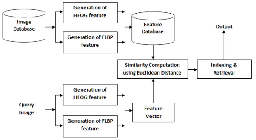
Here we have done two methods Histogram of Fuzzy Oriented Gradients and Fuzzy Local Binary Patterns. Shown in Figure 1.
Figure 1. CBIR System
2.1. Histogram of Fuzzy Oriented Gradient (HFOG)
Histogram of oriented gradient (HOG) feature descriptors was proposed by Dalal and Triggs [7]. The idea behind HOG descriptor is based on edge information. The HOG descriptor technique counts occurrences of gradient orientation in localized portions of an image detection window, or region of interest (ROI) [8].
The HFOG [9] should reflect a more objective description of content than the conventional HOG features. The main steps stays same as HOG in F-HOG. First, the image derivative in the horizontal and vertical directions are calculated, next step consists in computing the gradient and the magnitude of each pixel in the image. Then, contrarily to the standard HOG when each one of these pixels votes for a unique bin by adding its magnitude. Here belonging of a pixel in a bin is not obsolete. In this context, there will associate to each pixel a fuzzy description considering more than one bin; this represents the contribution of
the pixel into each one of these bins. Let I(x,y) be a pixel with a magnitude M(x,y) and a gradient 𝜃(x,y). In the original HOG, I(x,y) will belong only to the range [ ] where k is a positive integer belonging to [0; n] and n is the number of bins considered. In another words, the whole magnitude of the pixel I(x;y) will be added only to the range [ ]. However, in the proposed HFOG, based on the idea that a pixel gradient can belong to several bins at the same time, the magnitude of I(x;y) will be added to all these bins with a degree specified by membership grades between 0 and 1. For this purpose, a membership degree is defined using the Fuzzy membership function of Fuzzy-C-Means algorithm:
( )
∑ (‖ ‖
‖ ‖)
Where ( ) is the contribution of the pixel in in the value of the bin , and m is a parameter which controls the degree of fuzziness in the distribution of pixels (1 < m <1). Empirically, found that m=1.1 is the best setting. Once the degree of voting of a pixel on each bin is calculated, the magnitude of this pixel will be added to the bins, depending to the membership degree.
A. Algorithm: Fuzzy Local Binary Pattern Input: Query Image
Output: HFOG feature vector Steps:
1. Calculate the image gradient in X and Y directions.
2. Compute the gradient 𝜃 and magnitude of each pixel in the image.
3. Each one of these pixels votes for a unique bin according to the orientation of the pixel. i.e., (𝜃 ) values.
4. Calculate the average of each bin, i.e., 𝜃 .
5. Calculate contribution of each angle in the respective Bins, ( ). 6. Multiply ( ) with its magnitude M.
7. Scale the image in the range (0,250).
8. Find the normalized histogram which is the feature vector of the image. 9. Process is repeated for all images in the database and feature database is form. 10. Perform similarity computing.
2.2. Fuzzy Local Binary Patterns (LBP)
Local binary patterns were introduced by Ojala et al [10] as a fine scale texture descriptor. Local Binary Pattern (LBP) [10] is a simple yet very efficient texture operator which labels the pixels of an image by thresholding the neighborhood of each pixel and considers the result as a binary number. Due to its discriminative power and computational simplicity, LBP texture operator has become a popular approach in various applications. It can be seen as a unifying approach to the traditionally divergent statistical and structural models of texture analysis. Perhaps the most important property of the LBP operator in real-world applications is its robustness to monotonic gray-scale changes caused, for example, by illumination variations. Another important property is its computational simplicity, which makes it possible to analyze images in challenging real-time settings.
LBP description of a pixel is created by thresholding. The values of the 3X3 neighborhood of the pixel against the central pixel and interpreting the result as a binary number.
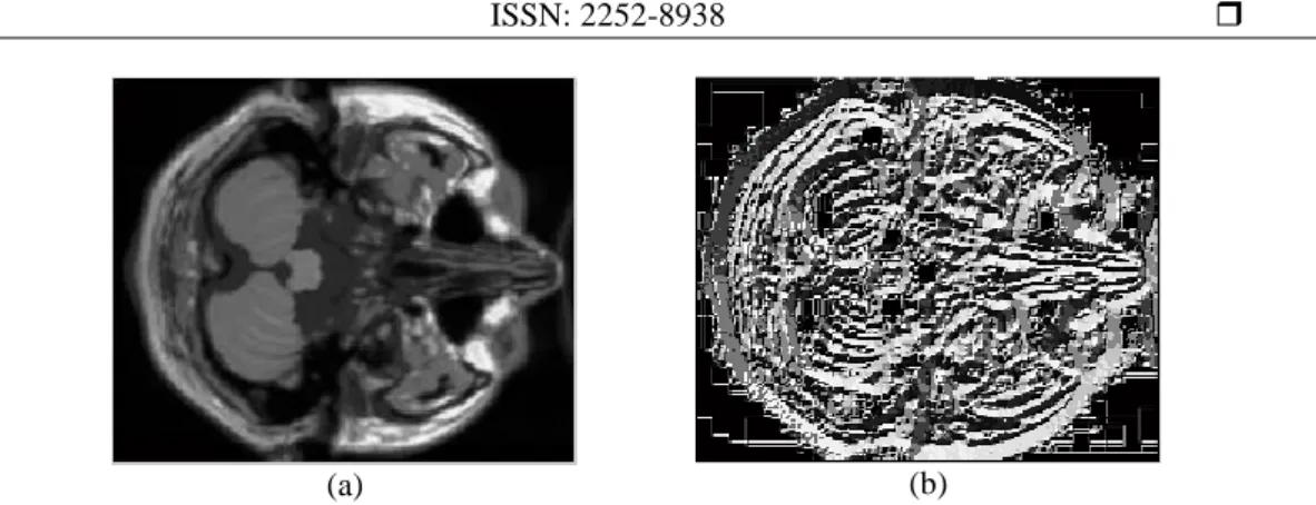
The original LBP is based on hard thresholding the neighborhood of each pixel, which makes texture representation sensitive to noise. In addition, LBP cannot distinguish between a strong and a weak pattern. In order to enhance the LBP approach [11], Fuzzy Local Binary Patterns (FLBP) [12] is proposed. In FLBP, any neighborhood does not represented only by one code, but, it is represented by all existing codes with different degrees. In FLBP, any fuzzy Intersection and Union operators may be used. Shown in Figure 2.
(a) (b) Figure 2. Query Image and its Corresponding LBP Pattern
The fuzzification of the LBP approach [12] includes the transformation of the input variables to respective fuzzy variables, according to a set of fuzzy rules. For this purpose, two fuzzy rules are introduced to describe the relation between the intensity values of the neighborhood pixels and the central pixel
as follows:
According to the above rules, two membership functions, m0 and m1, are needed. Let functions m0 and m1 define the degree to which is 0and 1, respectively. The m0 should be descending with respect to . Therefore, as a membership function m0, we consider the decreasing function defined in equation below:
( ) {
On the other hand, membership function m1 defines the degree to which is 1. This function may be the complement of$ m0. i.e.,
( ) ( )
For both m0 and m1, T [0, 255] represents a parameter that controls the degree of fuzziness.
Figure 3. Membership Functions m0 and m1 as a Function of Pi – Pcentre
Although for the original LBP operator a single LBP code characterizes a neighborhood, but, in the proposed FLBP approach, a neighborhood may be characterized by all available LBP codes on di_erent membership degrees. The membership degree of each LBP code in a pixel depends on the membership functions m0 and m1 shown in Figure 3, and all neighborhood values of the pixel. For any neighborhood, the contribution CLBP of each LBP code is defined as:
⋂ ( )
where [ ] is a LBP code and is the bit of it. Also, is the intersection (AND) operator. After computing the contribution of the LBP codes in all of the pixels, a histogram can be defined as:
⋃ ( )
where is the union operator. This FLBP histogram contains information about the distribution of the local micropatterns, such as edges, spots and flat areas over the whole image, so can be used to statistically describe the image characteristics.
B. Algorithm: Fuzzy Local Binary Pattern Input: Query Image
Output: FLBP feature vectorSentence_TDW_Feature =Preprocessing (W); Steps:
1. Determine the dimensions of the input image.
2. Block size, each LBP code is computed within a block of size bsizey*bsizex 3. Calculate dx and dy. dx = xsize-bsizex, dy = ysize-bsizey.
4. Fill the central pixel matrix C. 5. Initialize the result matrix with zeros.
6. Compute the neighbour image using the rules R0 : . .
7. Calculate m0 and m1, ( ) {
and ( ) ( ).
8. For all neighbourhoods assign contribution to histogram.
⋂ ( )
9. Calculate the histogram, which is the feature vector of the image.
⋃ ( )
10. Process is repeated for all images in the database and feature database is form. 11. Perform similarity computing.
2.3. Similarity Measure
For comparing the similarity of two metric we use Euclidean distance. In Cartesian coordinates, if p = (p1, p2,..., pn) and q = (q1, q2,..., qn) are two points in Euclidean n-space, then the distance (d) from p to q,
or from q to p is given by the Pythagorean formula:
( ) √∑( )
2.4. Performance Evaluation
Average Rank: Average rank is calculated using the images retrieved based on a set of random number of query images. In perfect case its value is 1 i.e., relevant images are in a succeeding order without the presence of irrelevant images in between them. Average rank is calculated using the formula:
(∑ ( )
)
3. RESULTS AND ANALYSIS
In our experiment, different types of axial view of brain image datasets are used, which is downloaded from publicly available BrainWeb dataset [http://brainweb.bic.mni.mcgill.ca/]. The data set consists of 150 T1 weighted images with 1 mm slice thickness, different noise levels (0%, 1%, 3 %, 7%, 9%) and different intensity non-uniformity (0%, 20%, 40%).
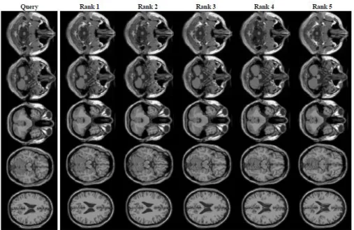
Figure 4. Query Image and 5 Relevant Images
3.1. Result of Histogram of Fuzzy Oriented Gradients
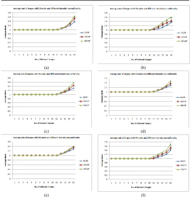
In Figure 4, the average rank verses number of images retrieved in different noise levels of Histogram of Fuzzy Oriented Gradients are shown. Figure 5(a) shows average rank in retrieving first 15 relevant images with 0% noise and 0%, 20% and 40% intensity non-uniformity. Figure 5(b) shows average rank of images with 1% noise and 0%, 20% and 40% intensity non-uniformity. Figure 5(c) shows average rank of images with 3% noise and 0%, 20% and 40% intensity non-uniformity. Figure 5(d) shows average rank of images with 5% noise and 0%, 20% and 40% intensity non-uniformity. Figure 5(e) shows average rank of images with 7% noise and 0%, 20% and 40% intensity non-uniformity And Figure 5(f) shows average rank of images with 9% noise and 0%, 20% and 40% intensity non-uniformity. By analyzing these results there can be concluded that as intensity non-uniformity increases performance decreases slightly.
(a) (b)
(c) (d)
(e) (f)
Figure 5. Average Rank verses the Number of Relevant Images Retrieved with Different Noise Levels and Different Intensity Non-uniformity (“RF”) with HFOF
3.2. Result of Fuzzy Local Binary Patterns
In figure 5, the average rank verses number of images retrieved in different noise levels of Fuzzy Local Binary Patterns are shown. Figure 6(a) shows average rank in retrieving first 15 relevant images with 0% noise and 0%, 20% and 40% intensity non-uniformity. Figure 6(b) shows average rank of images with 1% noise and 0%, 20% and 40% intensity non-uniformity. Figure 6(c) shows average rank of images with 3% noise and 0%, 20% and 40% intensity non-uniformity. Figure 6(d) shows average rank of images with 5% noise and 0%, 20% and 40% intensity non-uniformity. Figure 6(e) shows average rank of images with 7% noise and 0%, 20% and 40% intensity non-uniformity And Figure 6(f) shows average rank of images with 9% noise and 0%, 20% and 40% intensity non-uniformity. By analyzing these results there can be concluded that as intensity non-uniformity increases performance decreases slightly.
(a) (b)
(c) (d)
(e) (f)
Figure 6. Average Rank verses The Number of Relevant Images Retrieved with Different Noise Levels and Different Intensity Non-Uniformity (“RF”) with FLBP
3.3. Comparison of HFOG and FLBP
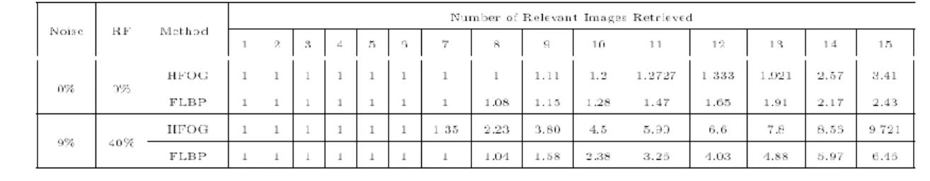
In Table I indicates the comparison of HFOG and FLBP for the retrieval of 15 relevant images. It also uses the same dataset used above. From the Table 1 and Figure 7 we can conclude that HFOG outperforms FLBP.
Figure 7. Comparison of HFOG and FLBP
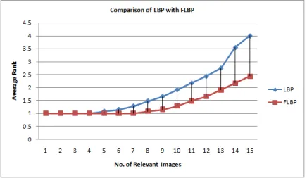
3.4. Comparison of LBP and FLBP
Figure 8 shows comparison of HFOG and FLBP. From there both of them gives good result but HFOG outperforms FLBP slightly.
Figure 8. Comparison of LBP and FLBP
4. CONCLUSION
Here proposes two methods, Histogram of Fuzzy Oriented Gradients and Fuzzy Local Binary Pattern for Brain MR Image retrieval. It is proven that HOG is a good descriptor for brain Image retrieval. In HOG, larger the number is more accurate the descriptor is. But the impact of the bin number affects the distribution of the histogram. So, here come to the concept of Histogram of Fuzzy Oriented Gradients. In HFOG each pixel belonging more than one bin at the same time with different degrees. Similarly fuzzification allows a Fuzzy Local Binary Pattern (FLBP) to contribute to more than a single bin in the distribution of the LBP values used as a feature vector.
REFERENCES
[1] Smeulders, M Worring, S Santini, A Gupta, R Jain, Content based image retrieval at the end of the early years.
Pattern Analysis and Machine Intelligence, IEEE Transactions on. 2000; 22: 1349-1380.
[2] Zukuan, WEI, et al. An Efficient Content Based Image Retrieval Scheme. TELKOMNIKA Indonesian Journal of Electrical Engineering. 2013;11(11): 6986-6991.
[3] Müller, Henning, Thomas M Deserno. Content-based medical image retrieval. Biomedical Image Processing.
[4] Lehmann, Thomas M, et al. Content-based image retrieval in medical applications: a novel multistep approach. Electronic Imaging. International Society for Optics and Photonics, 1999.
[5] Xia, Ling, et al. Medical Image Retrieval Based on Shape Features in DCT Domain. TELKOMNIKA Indonesian Journal of Electrical Engineering 2014; 12(2): 1116-1124.
[6] Felipe, Joaquim Cezar, Agma JM Traina, Caetano Traina Jr. Retrieval by Content of Medical Images Using Texture for Tissue Identification. Computer-Based Medical Systems, 2003. Proceedings. 16th IEEE Symposium. IEEE, 2003.
[7] Dalal, Navneet, Bill Triggs. Histograms of Oriented Gradients for Human Detection. Computer Vision and Pattern Recognition, 2005. CVPR 2005. IEEE Computer Society Conference on. IEEE, 2005; 1.
[8] Overett, Gary, Lars Petersson. Large Scale Sign Detection Using HOG Feature Variants. Intelligent Vehicles Symposium (IV), IEEE, 2011.
[9] Salhi, Abdel Ilah, Mustapha Kardouchi, Nabil Belacel. Histograms of Fuzzy Oriented Gradients for Face Recognition. Computer Applications Technology (ICCAT), International Conference on. IEEE, 2013.
[10]Ojala, Timo, Matti Pietikäinen, Topi Mäenpää. Multiresolution gray-scale and rotation invariant texture classification with local binary patterns. Pattern Analysis and Machine Intelligence, IEEE Transactions on 2002; 24(7): 971-987.
[11]Brahnam, Sheryl, et al. Localbinary patterns: new variants and applications. Springer Berlin Heidelberg, 2014. [12]Iakovidis, Dimitris K, Eystratios G Keramidas, Dimitris Maroulis. Fuzzy local binary patterns for ultrasound texture
characterization. Image Analysis and Recognition. Springer Berlin Heidelberg, 2008: 750-759.
BIOGRAPHIES OF AUTHORS
Ms. Athira T R, PG Scholar in Adi Shankara Institute of Engineering and Technology, specialization in CSE under MGU. B.Tech. degree in Computer Science Engineering from MGU, India, in 2013.
Dr. Abraham Varghese, presently working as an Associate professor in Department of Computer Science and Engineering, Adi Shankara Institute of Engineering and Technology. Completed PhD from Anna university Chennai and M.Tech (CSE) from National institute of Technology Karnataka (NITK), Surathkal. He has ten year experience in teaching and five year experience in research.