Information design through scarcity and social learning
∗
Alexei Parakhonyak
†and Nick Vikander
‡February 2019
Abstract
We show that a firm may benefit from strategically creating scarcity for its product,
in order to trigger herding behavior from consumers in situations where such behavior is
otherwise unlikely. We consider a setting with social learning, where consumers observe
sales from previous cohorts and update beliefs about product quality before making their
purchase. Imposing a capacity constraint directly limits sales but also makes information
coarser for consumers, who react favorably to a sell-out because they only infer that demand
must exceed capacity. Neither large cohorts nor unbounded private signals guarantee
efficient learning, because the firm acts strategically to influence the consumers’ learning
environment. Our results show that capacity constraints can serve as a practical tool for
information design: if private signals are not too precise and capacity can be changed over
time, then in large markets the firm’s optimal choice of capacity delivers the same expected
sales as the Bayesian persuasion solution.
JEL classifications: D21, D82, D83
Keywords: social learning, information design, capacity, Bayesian persuasion
∗A previous version of this paper was circulated until the title ‘Inducing Herding with Capacity Constraints’.
The paper has benefited from discussions with Nemanja Antic, James Best, Itai Arieli, Vincent Crawford, Nicolas Drouhin, Andrea Galeotti, Ben Golub, Paul Heidhues, Stephan Lauermann, Ignacio Monz´on, Steven Morris, David Myatt, Marek Pycia, Gosia Poplawska, Daniel Quigley, Larry Samuelson, Peter Norman Sørensen, Ran Spiegler, Bruno Strulovici, Balazs Szentes, Curtis Taylor, Marta Troya-Martinez, and participants of the Oxford Economic Theory Workshop, Game Theory Society World Congress (Maastricht 2016), EARIE (Lisbon, 2016), Transatlantic Theory Workshop 2016, Lancaster Game Theory Workshop 2016, International Industrial Organization Conference (Boston, 2017), the Royal Economic Society Annual Conference 2018, the XXXIII Jornadas de economia industrial 2018, the Midwest Economic Theory Conference 2018, as well as audiences in Cardiff, Gothenburg, and Copenhagen.
†University of Oxford, Department of Economics and Lincoln College. E-mail:
1
Introduction
This paper shows that firms may want to strategically create product scarcity, to influence
consumer learning in such a way that can effectively persuade consumers to buy. As is standard
in the literature on social learning (see foundational papers by Banerjee (1992) and Bikhchandani
et al. (1992)), each consumer receives a noisy private signal about product quality, but also infers
some information from observing earlier sales. To illustrate the mechanism at work, consider a
cohort of ten consumers who visit a firm, where each buys if and only if her signal was good.
A consumer who then arrives and observes initial sales of three may refuse to buy, even if her
own signal was good, because she infers that only three out of the ten others had a good signal.
But if the firm, without knowing product quality, had initially limited capacity to three sales
per period, then the consumer would observe a sell-out, and only infer that there were at least
three good signals. That may well convince the consumer to buy even if her own signal was
bad, and trigger a positive purchase cascade.
Now suppose that in our example, one out of ten consumers per period is perfectly informed
about quality, and that the firm is unconstrained. If quality is low, but say seven consumers
in period 1 receive good signals, then everyone will buy in period 2 except for the informed
consumer. The informed consumer’s choice not to buy will perfectly reveal low quality and lead
to zero sales in later periods. However, this same choice would not reveal any information if the
firm had restricted capacity, because the informed consumer would be effectively pooled with
those who were rationed.1
Thus, neither large cohort size (as in the ‘guinea pigs’ considered by Sgroi (2002)) nor
un-bounded signals (as in Smith and Sørensen (2000)) guarantees efficient social learning. The
reason is that here, the consumers’ learning environment is endogenous, and the firm can
ma-nipulate this environment by restricting capacity. The result is that consumers may fail to learn,
in particular in situations where learning would hurt the firm.
The attractiveness of restricting capacity as a tool to manipulate learning can be understood
1In the spirit of Smith and Sørensen (2000), we use the word ‘cascade’ to refer to a situation where all
more broadly in terms of information design. A firm’s choice of capacity affects the structure
of consumers’ public information, analogous to the way a sender determines the structure of a
receiver’s private signal in models of Bayesian persuasion. We show that in large markets, a firm’s
optimal capacity choice can deliver exactly the Bayesian persuasion outcome, and therefore result
in optimal information provision. Bayesian persuasion mechanisms generally raise two practical
concerns: how the signal space is determined and how a sender can commit to a particular signal
structure. Neither concern is an issue in our setting, as both the signal space and commitment
power follow naturally from the firm’s choice of capacity.
In this sense, our paper brings out a close connection between Bayesian persuasion and
social learning despite apparent differences between the two approaches. In the former, a sender
directly influence agent learning by designing statistical experiments. In the latter, agents
learn by observing each others’ actions which may reveal their private information. And yet,
in practice, a seller’s simple choice to restrict capacity can end up persuading consumers, by
marshalling the forces of social learning: consumers learn just as they would have, had the
sender designed an optimal experiment.
Our focus on sell-outs and scarcity fits in with evidence that demand for some products
seems to persistently far outstrip supply and that suggests a plausible cause is seller strategic
behavior. Shortages for ‘Beanie Babies’ were accompanied by extremely high demand from 1996
to 1999. Debo et al. (2012) argue that scarcity for these toys was largely induced by the firm
itself. Chicago magazine writes that scarcity was a marketing strategy chosen by Ty Warner,
the toys’ creator:
The toys easily supplanted other fads such as Ninja Turtles and Cabbage Patch dolls
partly because of Warner’s strategy of deliberate scarcity. He rolled out each one —
Spot the Dog, Squealer the Pig — in a limited quantity and then retired it.2
For high-end restaurants, tables at ‘Noma’ in Copenhagen remain notoriously difficult to
come by, and reported waiting times for ‘Damon Baehrel’ or ‘Club 33’ in the United States
2See: https://www.chicagomag.com/Chicago-Magazine/May-2014/Ty-Warner/, accessed on February 7,
range from ten to fourteen years. Music festivals, such as those in Roskilde and Reading, also
often sell out well in advance, year after year, with tickets for Glastonbury 2016 selling out in
just 30 minutes.3 Sell-outs are also common in professional sports, where the Boston Red Sox
enjoyed a sell-out streak that stretched from 2003 to 2013. In terms of performances, Courty
and Pagliero (2012) argue that concert promoters believe that empty seats would reveal negative
information to consumers, and therefore select venues and prices to make sellouts more likely.
In a similar spirit, ‘papering the house’ is a common practice where some consumers quietly
receive free tickets so as to fill empty seats. Our formal model does not capture all the richness
of these particular situations, but echoes the same broad idea: consumers may react favourably
to sellouts, and sellers may take into account when making their strategic choices.
Formally, we consider a model of social learning where cohorts of consumers arrive
sequen-tially at a seller and observe sales from previous periods. Informed consumers perfectly know
whether product quality is high or low, whereas uninformed consumers receive a private noisy
signal. Consumers in each cohort simultaneously choose whether to buy or take their outside
op-tion and then leave the game. Initially, without knowing its quality, the seller can set a capacity
constraint, where per period sales cannot exceed capacity. This constraint effectively coarsens
the information of consumers since they cannot observe the extent of any excess demand.
We show that the seller may find it profitable to restrict capacity even though the constraint
directly limits sales, because sell-outs drive up uninformed consumers’ willingness to pay. The
result can be a positive purchase cascade, where all consumers buy regardless of their signal,
which in particular generates excess demand in later periods. This excess demand can actually
benefit the seller, if quality is in fact low, by masking the actions of informed consumers who
choose not to buy, thereby allowing the cascade to be maintained. Restricting capacity tends
to help in situations that a priori seem grim, where the product likely has low quality.
Thus, while our formal analysis does not consider dynamic pricing, our framework provides
a rationale as to why firms may not increase prices despite regular sellouts and likely excess
demand. To maximize expected profits, in the presence of demand uncertainty, it would often
3See http://www.glastonburyfestivals.co.uk/glastonbury-2016-tickets-sell-out-in-30-minutes/, accessed on
seem reasonable to charge a price that is high enough to prevent sellouts fromalways occurring.
Our analysis points out a downside to such a strategy, namely that a failure to sell out can
reduce future profits by stopping a positive purchase cascade.
We then explore how restricting capacity performs relative to Bayesian persuasion, i.e. ex
ante commitment to a rule that maps product quality to a binary purchase recommendation,
where each consumer decides whether to buy based on the recommendation and on her private
signal. We show that if private signals are relatively imprecise, then the optimal mechanism
gives consumers a recommendation to buy whenever quality is high, and sometimes when quality
is low. All consumers follow these recommendations regardless of their private signal.
Using the optimal mechanism as a benchmark, we consider the optimal choice of capacity
for a seller interested only in its informational impact. Here we abstract away from the cost
of restricting capacity, by allowing the seller to remove its constraint following a sellout and
assuming it is patient enough to only care about long-run expected sales. It turns out that if the
market is large, then the optimal capacity constraint yields long-run sales that are asymptotically
equivalent to those under the above-mentioned persuasion mechanism.
Our paper contributes to the literature on social learning with imperfect observability of past
actions. Different work has assumed that agents can observe a random sample of actions that
is anonymous (Banerjee and Fudenberg (2004), Smith and Sorensen (2013), Monz´on and Rapp
(2014), Monz´on (2017)) or non-anonymous (Acemoglu et al. (2011), Lobel and Sadler (2015)),
the aggregate total of all past actions (Callander and H¨orner, 2009), the aggregate total of one
particular action (Guarino et al. (2011), Herrera and H¨orner (2013)), or only the choice of an
agent’s immediate predecessor (C¸ elen and Kariv, 2004). Unlike these papers, the information
structure in our setting is endogenous, so consumers may fail to learn about low quality despite
two features that the literature suggests should promote learning: multiple consumers who do
not have access to social information (see Banerjee (1992), Sgroi (2002), Acemoglu et al. (2011),
Smith and Sorensen (2013), Golub and Sadler (2017)); and unbounded private signals (see, e.g.,
Smith and Sørensen (2000), Banerjee and Fudenberg (2004)).
and Gentzkow (2011). As our seller can only influence consumers’ information through its choice
of capacity, the paper complements work looking at a sender’s choice from a restricted set of
signal structures: Tsakas and Tsakas (2017) consider noise that distorts signal realizations,
Perez-Richet and Skreta (2018) study sender manipulation of test results, and Ichihashi (2018)
focuses on which signal-structure restrictions are optimal for the receiver. In terms of costly
persuasion, Gentzkow and Kamenica (2016, 2017) and Mensch (2018) assume a direct cost
associated with each experiment, whereas our cost of restricting capacity (i.e. foregone sales)
is implicit and depends on consumer behavior. Other papers share our focus on dynamics (see
Au (2015), Ely (2017), Renault et al. (2017), Best and Quigley (2017), Bizzotto et al. (2018),
Orlov et al. (2018)), but none consider scarcity or social learning.4
A few recent papers consider information design as a way to influence social learning. Kremer
et al. (2014) and Che and H¨orner (2017) both look at settings where agents arrive sequentially,
and show that a designer looking to maximize total surplus may prefer an information structure
that is coarse, to encourage experimentation and promote learning. In contrast, we consider a
firm looking to maximize profits, and show that it may choose a coarse information structure
in order to limit learning.
Our results present a novel rationale for firms to strategically restrict capacity. Other work on
such scarcity strategies has mainly focused on discouraging consumer strategic delay (DeGraba
(1995), Nocke and Peitz (2007), M¨oller and Watanabe (2010)). In terms of scarcity and learning,
Debo et al. (2012) show that a firm may reduce service speed so that consumers observe longer
queues and infer higher quality. Stock and Balachander (2005) show consumers who observe
that inventory is low may infer that earlier demand (and hence quality) was likely high, which
can induce a firm to set low inventory. In contrast to our work, both papers assume the firm
is privately informed about quality, and scarcity does not hide information from consumers in
these settings, but instead may help reveal it.5 The broader literature on how firms can influence
4The signal structure associated with a capacity constraint in our setting involves upper-tail censoring:
re-vealing precise information about the state if news is sufficiently bad (i.e. demand below a threshold value), and coarse information otherwise. Dworczak and Martini (2017), Kolotilin et al. (2017), and Kolotilin and Zapechel-nyuk (2018) all show that upper-tail censoring can at times be optimal in persuasion problems where the state is drawn from a continuous distribution.
consumer learning has mainly focused on pricing (Welch (1992), Bose et al. (2006), Bose et al.
(2008), Sayedi (2018)), rather than scarcity.6
We describe our model in Section 2. Section 3 present preliminary results regarding consumer
learning under restricted capacity, along with our key technical lemma, and Section 4 is devoted
to the baseline model where all consumers are uninformed. Section 5 asymptotically compares
the informational impact of capacity constraints to Bayesian persuasion. We extend the baseline
model in Section 6 to consider informed consumers, and Section 7 then concludes. All the proofs
are presented in Appendix A. Appendix B contains more general analysis of our deterministic
and stochastic models. Appendix C presents our results on pricing in the presence of capacity
constraints.
2
Model
Suppose there is a product or service of unknown quality and two possible states of the world,
Ω ={G, B}. In state G, quality is good and each consumer who buys obtainsuG = 1. In state
B, quality is bad and each consumer who buys obtains uB = 0. A consumer who does not buy
gets reservation utility r ∈(0,1).
The actual state is not initially known, neither to the seller nor to consumers. A priori beliefs
of all players are thatP(G)≡β andP(B) = 1−β. In each period there are 2npotential buyers,
who are either informed or uninformed. Before making her purchase decision, each informed
consumer receives a signal that reveals the state for sure. Each uninformed consumer receives
a noisy private signal, s ∈ {g, b}, where P(g|G) = P(b|B) ≡ α ∈ (1/2,1). By α < 1, our
signals are boundedly informative. We also assume that a consumer without further information
would follow her signal, i.e. P(G|s =g)> r > P(G|s =b). We model the number of informed
consumers in two ways. In the deterministic setting, we will assume there is a fixed number
m of informed consumers in every period, where 1 ≤ m ≤ n. In the stochastic setting, we
assumes bounded rationality and social image concerns.
6See also Gill and Sgroi (2008) on product testing, Gill and Sgroi (2012) on choice of reviewers, and Aoyagi
will assume that each of the 2n consumers is informed with probability ε > 0.7 We will also
consider a baseline where all consumers are uninformed, which would correspond to imposing
m= 0 or ε= 0 in the deterministic or stochastic settings.
At the start of the game, t = −1, the seller can set a capacity constraint K ≤ 2n. This
capacity choice is irreversible and limits potential sales in each period (i.e. how many consumers
can buy), which cannot exceed capacity. The state of the world is realized at t = 0, so the
constraint itself does not reveal any information.8
In each period t ∈ [1,∞), 2n consumers arrive and observe both capacity and total sales
from the consumers in previous cohorts. That is, consumers do not directly observe quantity
demanded in each period, but only quantity sold. Notice that a sell-out in period t0 < t, where
sales equal capacity, need not imply that demand precisely equaled capacity.
Each of the 2n consumers who arrive in period t choose whether they want to buy based
on (i) prior beliefs about quality, β, (ii) a private signal, s, and (iii) observed sales from the
previous cohorts.9 The decision of informed consumers is solely determined by their signal. If
more than K consumers want to buy in period t, a random selection of them are served, and
the remaining consumers use their outside option. All period-tconsumers then leave the market
forever, and a new cohort of 2n consumers arrives in periodt+ 1.
The seller receives a fixed profit per consumer who buys, normalized to 1. He discounts
profits in future periods with a factor of δ, and sets K so as to maximize expected discounted
future profits.
7Our approach of modeling unboundedly informative signals, through the presence of fully informed
con-sumers, differs from the more common approach of assuming continuous signals, and dramatically helps with tractability.
8Parsa et al. (2005) document that about 60% of new restaurants fail within three years, which suggests that
their owners had imprecise information about quality when opening and setting capacity. Ultimately, we require that the seller and consumers holds the same prior, as is common in the literature on social learning, see, e.g., Bose et al. (2006), Bose et al. (2008) and Bhalla (2013).
9In our setting it does not matter how long a history is observed, provided that consumers observe at least
3
Preliminary Results
3.1
Consumer Behaviour
Define Qi
ω(j) as the probability of j good signals from 2n consumers in period 1, conditional
on the state being ω ∈ {G, B} , in either the deterministic (denotei=det), stochastic (denote
i=sto), or baseline (denotei=base) setting. In the deterministic setting,mconsumers receive
a correct signal for sure, and the remaining 2n−mconsumers each receive a correct signal with
probability α, which implies
QdetG (j) =
2n−m j −m
αj−m(1−α)2n−j, (1)
if j ≥m, and Qdet
G (j) = 0 if j < m, along with
QdetB (j) =
2n−m j
α2n−m−j(1−α)j, (2)
if j ≤2n−m and Qdet
B (j) = 0 if j >2n−m.
In the stochastic setting, each consumer receives a correct signal with probability+(1−)α,
where is the probability of being informed. This implies:
QstoG (j) =
2n j
[1−(α+ε−αε)]2n−j(α+ε−αε)j, (3)
QstoB (j) =
2n j
[1−(α+ε−αε)]j(α+ε−αε)2n−j. (4)
The baseline probabilities Qbaseω (j) can be obtained by setting m =ε = 0 in the above
expres-sions. We also introduce an unconditional probability of havingj good signals
Qi(j) =βQiG(j) + (1−β)QiB(j), j ∈ {base, det, sto}
We start by showing that Qi
ω(j) exhibits the following four properties.
{G, B}, i∈ {base, det, sto}, satisfy the following conditions:
(i) QiB(j) Qi
G(j)
is non-increasing in j.
(ii) QiB(n) Qi
G(n)
= 1, QiB(n−1) Qi
G(n−1)
≥ α
1−α 2
and QiB(n+1) Qi
G(n+1)
≤ 1−α α
2 .
(iii) Qi
B(j) =QiG(2n−j) for all j ≤2n.
(iv) QiG(j)> QiG(2n−j) if j ≥n+ 1.
That is, (i) more good signals means the good state is more likely, (ii) having an equal
number of good and bad signals is just as likely in either state, and the smallest difference from
an equal number is sufficiently informative, (iii) j good signals in the bad state is as likely as j
bad signals in the good state, and (iv) in the good state, j ≥ n+ 1 good signals is more likely
than j bad ones.
In what follows we assume that consumers follow their private signals in the absence of other
information, i.e. P(G|s=g)> r > P(G|s =b), or
βα
βα+ (1−β)(1−α) > r >
β(1−α)
β(1−α) + (1−β)α. (5)
Now we formulate the optimal behaviour for a consumer in period tfacing an unconstrained
seller, following a sequence of sales (S1, . . . , St−1).
Lemma 2. Suppose the seller is unconstrained and consider an uninformed consumer A acting in period t≥2. Then in the baseline, deterministic, and stochastic settings:
1. If t = 2 or t >2 and Sτ =n for all τ ≤t−1:
(a) if St−1 > n then A buys regardless of her own signal;
(b) if St−1 =n then A follows her own signal;
(c) if St−1 < n then A does not buy regardless of her own signal.
(a) if St−1 = 2n, then A buys regardless of her own signal;
(b) if St−1 <2n then A does not buy regardless of her own signal.
3. If t >2 and maxτ≤t−2Sτ < n:
(a) if St−1 >0, then A buys regardless of her own signal;
(b) if St−1 = 0 then A does not buy regardless of her own signal.
Following the literature on social learning, Lemma 2 describes optimal behavior on the
equilibrium path; we do not specify consumers’ beliefs and best responses for histories which
cannot arise from equilibrium behaviour. As each consumer’s payoff does not depend on the
actions of those who follow, this approach is not restrictive. The idea of Lemma 2 is that initial
sales of at least n+ 1 out of 2n is sufficiently good news to trigger a positive purchase cascade
where all uninformed consumers buy. This cascade continues unless (or until) there is a period
with fewer than 2n sales, which would reveal that an informed consumer chose not to buy, and
that the state was actually bad. This would in turn trigger a negative cascade. The story is
similar for sales of at mostn−1 in period 1, which triggers a negative cascade where uninformed
consumers do not buy, unless (or until) there is a period with strictly positive sales.
Now we look into consumer behaviour when the seller restricts capacity. It follows from
Lemma 2 that a capacity K ≥ n+ 1 limits sales compared to being unconstrained, but does
not increase the probability of starting a positive cascade. As such, we will focus on levels of
capacity K ≤n in our analysis. Moreover, setting capacity very low means that multiple
sell-outs may be necessary to trigger a cascade: say, selling out a restaurant of one seat given one
hundred potential customers has very little impact on consumers’ beliefs. However, as Lemma
3 will establish, consumers become increasingly optimistic after each sell-out.
Consider a consumer in cohort l+ 1 who receives a bad signal, realizes there were sell-outs
in all l previous periods, and believes that all earlier consumers followed their private signals.
γ(l, K) = P(G∩b, l sell-outs)
P(G∩b, l sell-outs) +P(B∩b, l sell-outs) =
β(1−α)
h P2n
j=KQ i G(j)
il
β(1−α)hP2n j=KQ
i G(j)
il
+ (1−β)αhP2n j=KQ
i B(j)
il =
1
1 + 1−ββ α
1−α hP2n
j=KQiB(j) P2n
j=KQiG(j)
il (6)
where i∈ {base, det, sto}.
Lemma 3. In the baseline, deterministic, and stochastic settings, for all 1≤K ≤n, consumer beliefs γ(l, K) are increasing in l, with liml→∞ γ(l, K) = 1.
As beliefs γ(l, K) are increasing in l, a sufficiently long sequence of sell-outs will eventually
lead to a positive purchase cascade. We use the results of Lemma 3 for our derivation of general
profit functions and analysis of social learning in the long run. There we illustrate that a seller
might sometimes prefer to set a low capacity that delays the start of a positive cascade. That
being said, we now show that for all parameter values satisfying our assumptions, there is always
a value of the outside optionr such that a cascade is triggered by a single sell-out.
Lemma 4. In the baseline, deterministic, and stochastic settings, for all K ≤ n there exists
r∈(0,1) such that γ(1, K)> r > γ(0, K) = P(G|s =b).
We will apply Lemma 4 for establishing our main existence result, i.e. that for some
param-eter values the seller prefers to restrict capacity.
3.2
Key Lemma
Our aim is to show that there is a range of parameters in all settings such that the seller wants to
restrict its capacity. Moreover, we show that each value of K ≤n can sometimes lead to higher
essential for proving our main theorems in Sections 4 and 6. Let Q= {Q(j), 0≤ j ≤ 2n} be
a discrete probability measure: Q(j)∈[0,1] and P2n
j=0Q(j) = 1. This measure can correspond to that in any one of our settings described in Section 3.1, as well as in some alternative ones,
but at this point we are agnostic about the actual probabilistic model, so we do not use model
superscripts. Define
πuQ = 1 1−δQ(n)
2n X
j=0
jQ(j) + 2nδ 1−δ
2n X
j=n+1
Q(j)
!
, (7)
and
πcQ(K) = 2n X
j=0
min{j, K}Q(j) + Kδ 1−δ
2n X
j=K
Q(j), (8)
with δ∈(0,1).
Expressions (7) and (8) give seller profits assuming that cascades start upon a single sell-out
and, once started, continue forever. This is true in our baseline, but not in the deterministic or
stochastic setting. The following Lemma shows that if probabilitiesQsatisfy certain properties,
the seller prefers to be constrained, provided that cascades continue forever. Later, in the proofs
of the corresponding theorems, we will show that (i) parameters of the model can be chosen
such that Qi(j), i ∈ {base, det, sto} satisfy the properties required by Lemma 5, and (ii) the
assumption that cascades continue forever understates the seller’s incentive to restrict capacity
for i∈ {det, sto}.
Lemma 5. Consider a sequence of probability measures{Qs}∞
s=0 such thatlims→∞ Q s(n) P2n
j=n+1Qs(j)
= ∞. Then, there exist δ and T0, such that for all s > T0, n >1, K ≤n
πuQs < πcQs(K)
Suppose furthermore that lims→∞Qs(n) = 0. Then, for any δ ∈ q
2n−K
2n ,1
, there exists T1
such that for all s > T1 we have πQ
s u < πQ
4
Baseline Setting
4.1
Main Results
We start our analysis with the baseline and look into the seller’s incentives to restrict capacity.
We define acorrect cascade as a situation where all consumers buy regardless of their signal and
the state is good, or where they all refuse to buy regardless of their signal and the state is bad.
We define anincorrect cascade as a situation where all consumers refuse to buy and the state is
good, or where they all buy and the state is bad.
Profits for an unconstrained seller are
πbaseu = 2n X
j=0
jQbase(j) +δQbase(n)πu+δ
2n X
j=n+1
Qbase(j) 2n
1−δ, (9)
with Qbase(j) being probabilities in the baseline case. Period-1 sales of strictly more (less) than
n immediately trigger a positive (negative) cascade, which continues in all later periods.
According to Lemma 4, there are values of r for which a single sell-out generates a cascade.
For such values of r, profits for a seller with capacity constraintK ≤n are
πcbase(K) = 2n X
j=0
min{j, K}Qbase(j) +δ
2n X
j=K
Qbase(j) K
1−δ. (10)
Notice that (9) and (10) correspond to (7) and (8), if we set Q(j) = Qbase(j) in the latter two
expressions.
Theorem 1. For any n >1, K ≤n and δ >
q
2n−K
2n , there are (α, β)∈(1/2,1)×(0,1/2) and
r > 0 for which the seller can increase its profits above the unconstrained level by restricting
capacity to K.
The seller faces a tradeoff, as restricting capacity limits sales in each period, but also increases
the probability of a positive cascade. A key difference between (9) and (10) is that below
average period-1 demand, between K and n, can only trigger a positive cascade if the seller is
cascade occurs after a single sell-out. Intuitively, having set a capacity constraint will tend to
help the seller when the state turns out to be bad, because the constraint can hide information
from consumers. The seller effectively engages in obfuscation, which increases the probability
of an incorrect positive cascade (where all consumers buy despite the state being bad) and
decreases the probability of an incorrect negative cascade (where no consumer buys despite the
state being good).
Having shown that the seller may sometimes find it profitable to restrict capacity, we now
say something about the conditions under which this can occur. Consistent with the above
intuition, the seller will only restrict capacity if it is sufficiently likely that the state is bad.
Proposition 1. Suppose that β ≥1/2. Then for all parameter values, such that consumers in the first period follow their signals, the seller prefers not to restrict capacity: πbaseu > πbasec (K)
for all K ≤2n.
When the state is good, initial sales are likely to be sufficiently high to trigger a positive
cascade regardless of whether the seller restricts capacity, and an unconstrained seller then
enjoys higher sales. The proof shows that for β ≥ 1
2, the good state is sufficiently likely that expected sales for an unconstrained seller exceed n per period. This is more than the seller
could possibly earn per period by restricting capacity to K ≤ n, which are the only capacity
levels that can increase the probability of a positive cascade. The result of Proposition 1 does
not rely on the outside option satisfying Lemma 4, i.e. it holds regardless of whether a single
sellout is sufficient to trigger a cascade, or if multiple sellouts are necessary (see Section 4.2).10
The sufficient condition provided in Proposition 1 is simple and intuitive, but the necessary
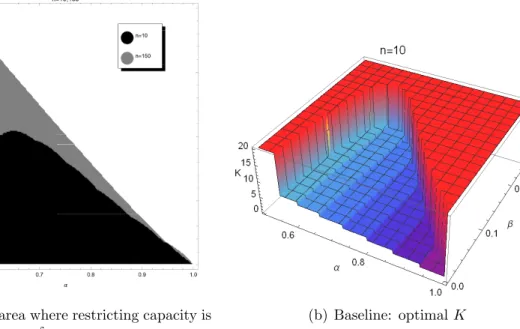
condition is much harder to obtain, so we investigate this question numerically. Figure 1(a)
shows that the region where restricting capacity can be optimal is larger when there are many
consumers. Intuitively, an increase in the number of consumers makes period-1 demand more
informative, so that an unconstrained seller is more likely to suffer a negative cascade in the
bad state. Restricting capacity then becomes more attractive, as a way to hide unfavourable
10A result similar to Proposition 1 can be obtained in the deterministic and stochastic models. The proof is
Figure 1: Areas where capacity restriction can be optimal.
(a) Baseline: area where restricting capacity is optimal for somer, δ
(b) Baseline: optimalK
information from consumers.
Figure 1(a) also shows an interesting interaction between signal precision and the prior.
When the signal is very imprecise (α ≈ 1/2), at least half of the consumers will likely buy,
regardless of the state, so the seller will remain unconstrained and bet on generating a positive
cascade. As signal precision increases, an unconstrained seller becomes increasingly likely to
experience a negative cascade when the state is bad, so the seller will restrict capacity for
sufficiently smallβ. A further increase in signal precision makes restricting capacity increasingly
helpful in the bad state, but increasingly harmful in the good state, as a correct positive cascade
is then likely without a constraint. The first effect dominates for intermediateα, but the second
effect dominates whenα is sufficiently large, because an incorrect positive cascade is only likely
given a very low constraint, which would dramatically reduce profits in the good state. Figure
1(b) depicts the optimal level of capacity for these different parameter values.
In our analysis, we assumed that the seller cannot adjust capacity over time, but this
as-sumption is not crucial. A seller that could adjust its capacity would effectively remove the
re-sult that restricting capacity can be optimal, as future gains following a cascade would no longer
be bounded by the size of the initial constraint. If the seller found it optimal to restrict capacity
in our setting, then it would also do so if capacity could be adjusted over time. Moreover, the
effective cost of setting a low constraint would be limited to a single period, so the seller would
be more aggressive in period 1 in order to make a sellout more likely, and then capture the
resulting gains. The following Proposition formally describes this result.
Proposition 2. Suppose thatK1 is the optimal period-1 capacity constraint when the seller can
adjust capacity over time, and that K0 is the optimal constraint when the seller cannot do so.
Suppose furthermore that selling out once at either K0 or K1 triggers a positive cascade, i.e.
min{γ(1, K0), γ(1, K1)} ≥r. Then K0 ≥K1.
4.2
General Profit Functions
The profit function (10) for a constrained seller applies to situations where a single sell-out
triggers a positive cascade. For given prior beliefs, signal accuracy, and capacity, we can always
find a value of the consumers’ outside option such that one sell-out is indeed sufficient. But more
generally, multiple sell-outs may be necessary to trigger a cascade, in particular when capacity
is relatively low. Might the seller have an incentive to set such a capacity, which delays the start
of a positive cascade, but also increases the probability of selling out?
To address this issue, we write down general profit functions for a seller with capacity K,
in the baseline setting. Recall from (6) that γ(l, K) denotes the belief of a consumer in cohort
l+ 1 that the state is good, after sell-outs in all l previous periods, and after receiving a bad
signal. Let L = {l : γ(l, K) > r}, which is non-empty by Lemma 3, and denote the smallest
element of L by L: the number of consecutive sell-outs required as of period 1, given capacity
K, in order to generate a positive cascade. The value of L is decreasing inK, since selling out
at higher capacity presents stronger evidence that the state is good.
Let ηω = P2n
j=KQ base
ω (j) denote the probability of a sell-out, given state ω ∈ {G, B}. Let
Sω = PK −1
j=0 jQ
base
ω (j) denote expected sales in a given period conditional on not selling out,
Figure 2: Seller profits and L.
0 2 4 6 8 10 K
2.0 2.2 2.4 2.6 2.8 3.0 3.2 π
n=10, m=0,δ=0.8,α=0.9,β=0.001, r=0.008
πU πC(K)
(a)
34
9
4 3
2 1 1 1 1 1
0 2 4 6 8 10 K 0
5 10 15 20 25 30 35
π
n=10, m=0,δ=0.8,α=0.9,β=0.001, r=0.008
L
(b)
Expected profits given capacity K and L≥1 are
πcbase(K) = β
1−(δηG)L
1−δηG
(SG+ηGK) + (δηG)L
K
1−δ
+
(1−β)
1−(δηB)L
1−δηB
(SB+ηBK) + (δηB)L
K
1−δ
. (11)
When the state is bad, the seller experiences L consecutive sell-outs each with probability
ηB, which triggers a positive cascade and yields revenue ofK in all periods. Otherwise, the seller
earns SB in the first period where it fails to sell out, and then zero in all later periods. The
situation is similar when the state is good, except the probability of a sell-out in each period
is ηG rather than ηB, and a seller that fails to sell out earns SG in that period. As expected,
expression (11) reduce to (10) if L= 1, so if one sell-out is sufficient to trigger a cascade.
Holding capacity constant atK, profits are strictly decreasing inL, because a largeLmeans
that more sell-outs are required to trigger a positive cascade. However, L depends on K, and
the seller may in fact want to set a sufficiently low capacity that results in L > 1. Such a low
capacity makes a sell-out in each period more likely, and thus reduces the probability in each
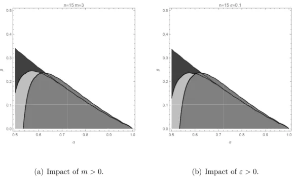
period that a negative cascade begins. Indeed, Figure 2 shows parameter values for which the
seller prefers to set K = 1, so that L= 34 sell-outs are necessary to trigger a cascade.
occur. An increase in K gives a lower chance of a sell-out in any given period, higher sales
conditional on selling out or on being in a positive cascade, and may also mean that fewer
sell-outs are necessary for the cascade to begin. The balance between these three forces may
sometimes swing sharply. In the figure, an increase in K from 5 to 6 reduces the number of
sell-outs necessary to start a cascade from L= 2 to L= 1, which pushes up profits.
5
Optimal Information Design
We now explore how the informational impact of restricting capacity, in terms of influencing
consumer behavior, compares to that of optimal information design. Our seller (sender) chooses
capacity without knowing the state, and each consumer (receiver) then receives information
that depends on the realized state and on capacity. In this sense, capacity constraints serve
as a natural example of a Bayesian persuasion mechanism that can be easily implemented in
practice. As capacity is chosen ex ante, and market participants do not observe excess demand,
any commitment problem in implementing the desired information structure is avoided. The
seller simply cannot serve demand that exceeds capacity. Consumers then directly observe the
resulting sell-out; if they did not, the seller could easily disclose that a sell-out occurred.
In what follows, we derive the optimal ‘persuasion mechanism’ in our setting, and then
examine how capacity constraints perform relative to this benchmark. The seller commits to a
rule which maps the binary state into a purchase recommendation. The state is realized, and
each consumer receives a recommendation according to the chosen rule. Each consumer then
makes a purchase decision based on the recommendation and her own private signal, and the
seller serves all consumers who want to buy. Thus, the seller’s persuasion mechanism substitutes
for the social learning process studied in the previous sections.
We consider information design without elicitation, where the same rule applies to all
con-sumers, regardless of their private signal. As Kolotilin et al. (2017) and Bergemann and Morris
(2017) show, given binary state and action spaces, this forms of information design is equivalent
As such, the rule we derive will constitute the optimal mechanism.11
The seller designs the persuasion mechanism to maximize expected sales, which are the
same in every period. When later making the comparison with capacity constraints, we will
assume that the seller is infinitely patient, and can adjust capacity over time. These
assump-tions effectively remove the direct cost of restricting capacity, i.e. limiting sales. The seller
will therefore set capacity to maximize long-run expected per-period sales, and have the same
objective function as in the persuasion setting.
The optimal persuasion mechanism is characterised by a binary message space corresponding
to the binary decision set of consumers (see Kamenica and Gentzkow (2011)). However, as
buyers are informed, the seller essentially chooses between three options. The first is where all
consumers follow the seller’s recommendation, which is the ‘textbook’ form of persuasion. The
second is where consumers with bad private signals always follow the seller’s recommendation,
but consumers with good signals ignore the recommendation and instead always buy. The third
is where all consumers ignore the recommendation, and follow their private signals.
We first consider a mechanism where all consumers follow the seller’s recommendation.
Sup-pose the seller sends a buy recommendation with probability pG in a good state and with
probability pB in bad state, and otherwise sends a no-buy recommendation. The belief of a
consumer with a bad signal upon receiving a buy recommendation is
γ(s=b, buy) = β(1−α)pG
β(1−α)pG+ (1−β)αpB
≥r,
which implies
β(1−α)(1−r)pG≥(1−β)αrpB. (12)
Clearly, if (12) is satisfied, then consumers with s =g prefer to buy. As both pG and pB enter
opposite sides of (12) with positive signs, setting
11We do not allow the seller to directly target different rules at consumers with different private signals. In
pG = 1, pB =
β(1−α)(1−r)
(1−β)αr , (13)
maximizes expected sales. Our assumption that a consumer would not buy, given only a bad
private signal, P(G|s=b)< r, implies pB<1, since
pB <1⇔β(1−α)(1−r)<(1−β)αr⇔
β(1−α)
β(1−α) + (1−β)α < r.
The seller always sends a buy recommendation in the good state, and only sometimes sends a
no-buy recommendation in the bad state, where the latter recommendation is perfectly revealing.
Echoing the discussion in Section 4 on restricting capacity, the seller effectively obfuscates when
the state is bad, by sometimes sending the same recommendation as when the state is good.
This recommendation convinces consumers to buy, even those with bad private signals. The
profits from this persuasion mechanism, per consumer and per period, are
π∗ =β+ (1−β)pB =β+
(1−α)(1−r)β
αr . (14)
Now consider a mechanism where only consumers with bad signals follow the seller’s
recom-mendation, and let (˜pG,p˜B) denote the probabilities of buy recommendations. The incentive
compatibility constraint for a consumer with a good signal who receives a no-buy
recommenda-tion is
γ(s=g, not buy) = βα(1−p˜G)
βα(1−p˜G) + (1−β)(1−α)(1−p˜B)
≥r,
or
βα(1−r)(1−p˜G)≥(1−β)(1−α)r(1−p˜B). (15)
Both (15) and (12) must bind at the optimum, which implies
˜
pG =
α(αβ−r(α(2β−1)−β+ 1))
(2α−1)β(1−r) , p˜B =
(1−α)(αβ −r(α(2β−1)−β+ 1))
The probability ˜pB is well-defined as long as ˜pG ∈[0,1]. This is the case if
α ≥α(r, β)≡ max{(1−r)β, r(1−β)}
r+β−2rβ , (17)
which is equivalent to condition (5), that consumers follow their private signals in the absence
of other information. The profits from this persuasion mechanism are
˜
π =β[α+ (1−α)˜pG] + (1−β)[αp˜B+ (1−α)]. (18)
As long as ˜pG,p˜B >0, these profits exceed βα+ (1−β)(1−α), which is what the seller would
earn if all consumers followed their private signals. Thus, the optimal mechanism either leads
all consumers to follow the seller’s recommendation, or only those with bad signals to do so.
Define
α(r)≡ 1 2
2r−1 +√4r2−8r+ 5, β(r)≡r2r−α(r)
3r−1 , β(r)≡
r
1−r[α(r) + 1−2r],
and note that 0< β(r)< r < β(r) for allr∈(0,1). The following Proposition establishes when
each of the two mechanisms yield higher profits, while taking into account constraint (17).
Proposition 3. For any r ∈ [0,1], if β ∈ [β(r), β(r)] and α ∈ [α(r, β), α(r)] then the optimal persuasion mechanism is given by (13). Otherwise, the optimal persuasion mechanism is given
by (16) as long as α > α(r, β).
Proposition 3 says that as long as signal precision is not too high, i.e. α ≤ α(r), the
optimal mechanism leads all consumers to follow the seller’s recommendation. The restriction
α ≥α(r, β) corresponds to our initial condition that consumers follow their own signals in the
absence of any other information. Finally, the restriction β ∈ [β(r), β(r)] guarantees that the
interval [α(r, β), α(r)] is non-empty.12
12Proposition 3 is similar to the result obtained in Kolotilin (2018), the only difference being that he also
Intuitively, for consumers with good private signals to ignore a no-buy recommendation,
the seller must sometimes send this recommendation in the good state, so the recommendation
is not perfectly revealing. The effective cost to the seller is that doing so reduces expected
sales in the good state, compared to a mechanism where consumers always follow the seller’s
recommendation. The size of this cost is decreasing in signal precision, because a consumer with
a very precise good signal may be willing to ignore a no-buy recommendation that suggests the
bad state is quite likely. In general, the scope for persuasion decreases as signals become more
precise: if α→1, then the expected profit of both mechanisms approaches β.
We now look into the optimal choice of capacity as a tool for information design. We again
assume that consumers observe sales from previous cohorts, and in particular whether a sellout
occurred. To ensure comparability with the optimal persuasion mechanism, we assume that
the seller is infinitely patient, and can costlessly adjust its capacity over time. The seller sets
its initial capacity to maximize expected per-period sales in the long run, which is equivalent
to maximizing the probability of a positive cascade.13 The question is how this probability
compares to that under the optimal persuasion mechanism, either (13) or (16).
First we focus on values of capacity K such that a single sellout triggers a positive cascade.
Recall thatηω(K,2n) = P2n
j=KQ base
ω (j) denotes the probability of sales greater than or equal to
K. A consumer with a bad private signal will buy after a single sellout if
β(1−α)ηG(K,2n)
β(1−α)ηG(K,2n) + (1−β)αηB(K,2n)
≥r,
or equivalently
β(1−α)(1−r)ηG(K,2n)≥(1−β)αrηB(K,2n). (19)
Constraint (19) resembles (12) but with one important difference: in the persuasion problem,
the seller can choosepGand pB independently, but now the choice of capacity jointly determines
both probabilities. The firm is interested in maximizing the probability of sell-out, so it will
choose the lowest K such that (19) is satisfied. Denote this value ofK by K∗(n).14
13If a positive cascade is triggered, the seller will immediately increase capacity and serve full demand. 14Note that for any n, we have η
Now we consider large cohorts. Note that limn→∞ηG(n,2n) = 1 and limn→∞ηB(n,2n) = 0.
Thus, for sufficiently largen, it must be the case thatK∗(n)< n, so that limn→∞ηG(K∗(n),2n) =
1; limn→∞ηB(K∗(n),2n) =
β(1−α)(1−r)
(1−β)αr <1, which is the same as the recommendation
probabil-ities in persuasion mechanism (13).
It follows that the limit result of restricting capacity is equivalent to the persuasion
mecha-nism where a buy recommendation is always sent in the good state and where consumers always
follow all recommendations. Here, a sellout always occurs in the good state and sometimes
occurs in the bad state, and it provides just enough good news to convince consumers to buy
regardless of their signal (i.e. a positive cascade). A failure to sell out perfectly reveals that the
state is bad, so that no consumer buys (i.e. a negative cascade).
We conclude that in large markets, the informational impact of the optimal capacity
con-straint serves as a good approximation to the above-mentioned persuasion mechanism. As this
mechanism is optimal when private signals are relatively imprecise, a seller can achieve optimal
information design in large markets with weak private information by restricting capacity to an
appropriate level.
One interpretation of the seller’s problem, as considered in this section, is in terms of trial
sales: the seller can first conduct a trial by making a limited number of units available of its
product, and then broadly release the product to all consumers if the trial goes well. Our results
suggest that in situations where private information is weak, the seller can do no better than
carrying out a single trial, then releasing the product broadly in the case of a sell-out, and
otherwise withdrawing the product from the market.
For completeness, we note that the optimal capacity constraint can never induce consumers
with good private signals to buy when the seller fails to sell out. Recall, thatK∗(n) is the
small-est capacity constraint to satisfy (19). Moreover, for K ∈ [K∗(n), n], we have that ηG(K,2n)
approaches 1 and ηB(K,2n) remains bounded away from 1 in a large market.15 Incentive
com-limn→∞ηB(n,2n) = 0, so K∗(n) exists for sufficiently large n. Finally, due to Lemma 1 part (i), K∗(n) is uniquely defined.
patibility for a consumer with a good private signal and a no-buy recommendation is
βα(1−r)[1−ηG(K,2n)]≥(1−β)(1−α)r[1−ηB(K,2n)],
which clearly cannot be satisfied as n approaches infinity, since the left-hand-side approaches
zero while the right-hand-side does not. Thus, in situations where (16) constitutes the optimal
persuasion mechanism, restricting capacity will result in inferior information design.16
We now use the above framework to say more about when the seller will restrict capacity
and the size of the optimal constraint. Clearly, a patient seller that can adjust its capacity
would never want to remain unconstrained in a large market. Period-1 sales would perfectly
reveal the true state, so an unconstrained seller would experience a correct positive cascade with
probability β,17 and an incorrect positive cascade with probability 0. In contrast, a seller that
restricts capacity will experience a correct positive cascade with probability β, and an incorrect
positive cascade with probability (1−β)ηB(K∗(n),2n))>0.
For the size of the optimal constraint, recall that limn→∞ηB(K∗(n),2n) = β(1(1−−αβ)(1)αr−r). The
left-hand side is directly decreasing in K∗, since a higher capacity reduces the probability of
selling out. Looking at the right-hand side, it follows that the size of the initial constraint set
by a patient seller that can adjust its capacity over time, in a large market, is decreasing in the
prior, β, and increasing in both signal precision, α, and the value of the outside option, r.
The idea is that a sellout at capacity K∗(n) hides just enough information about the bad
state to make a consumer with a bad private signal willing to buy. For such a consumer, a drop
say in signal precision makes buying more attractive. As a result the seller can hide on average
more unfavourable information by setting a lower capacity. Doing so makes it more likely to sell
out, and a single sellout will still generate a positive cascade.
The fact that the optimal capacity is increasing in signal precision stands in contrast with
16The key issue is that designing a persuasion mechanism involves two “degrees of freedom”, while setting a
capacity constraint involves only one. As a mechanism withpG = 1 is essentially a corner solution, any capacity sufficiently far below mean demand yields a sellout for sure in the good state, and the seller can set its exact capacity so as to best approximatepB. However, as ˜pG<1, this adds an extra binding constraint to the problem, which makes an approximation of (˜pG,p˜B) impossible.
Figure 1(b). What is the reason for this difference? In the current section, the outside option r
is fixed, and K∗(n) is the minimal capacity sufficient for triggering a cascade given the outside
option. Since the seller is patient, and can adjust capacity over time, its initial capacity choice
is essentially costless: it will set K =K∗(n) to maximize the probability of a positive cascade.
When plotting Figure 1(b), we allowed the outside optionrto vary, so that the minimal capacity
to trigger a cascade was always K = 1. We also assumed the seller could not adjust capacity
over time, which made setting K = 1 costly in terms of limiting future sales. As a result, the
seller often found it optimal to restrict capacity to a higher level, which was decreasing in signal
precision α.
If the seller sets low capacity K < K∗(n), then condition (19) will be violated, but Lemma
3 ensures a cascade will occur after a sufficiently long sequence of sellouts. For (α, β, r, n), and
any K, there exists l such that
β(1−α)(1−r)[ηG(K,2n)]l ≥(1−β)αr[ηB(K,2n)]l.
Following our earlier notation, let L denote the smallest integer l satisfying this inequality, so
that L sellouts are needed to trigger a positive cascade.
We now derive the long-run probability of a positive cascade in a large market, given low
capacity. Define Γ(l, K) as the public belief that the state is good, conditional on sell-outs at
capacity K in the first l ≤L periods. That is
Γ(l, K) = 1 1 + 1−ββ[ηB(K)]l
[ηG(K)]l
, (20)
where r < γ(L, K)<Γ(L, K) follows from (6) and the definition ofL. Moreover, we can write
β(ηG)L+ (1−β)(ηB)L
Γ(L, K) + 1−
β(ηG)L+ (1−β)(ηB)L
µ=β. (21)
The public belief conditional on an eventual positive cascade triggered byLsellouts, multiplied
negative cascade triggered by a failure to sell out in somel ≤Lperiod (denoted byµ), multiplied
by the probability of such a cascade; must equal the prior β.
By Lemma 1, high sales provide good news about the state, so for any fixed K we have
µ < Γ(L−1, K)Q
base
G (K−1)
Γ(L−1, K)Qbase
G (K−1) + [1−Γ(L−1, K)]QbaseB (K −1)
=
1
1 + [1−Γ(L−1,K)]QbaseB (K−1)
Γ(L−1,K)Qbase G (K−1)
. (22)
The average public belief, conditional on failing to sell out in one of the first L periods, cannot
exceed the public belief after selling out in exactlyL−1 periods, and then having period-Lsales
of K−1, only 1 below capacity. By the definition of L, a consumer who observesL−1 sellouts
will not buy if she receives a bad private signal. This implies that
Γ(L−1, K)(1−α)
Γ(L−1, K)(1−α) + (1−Γ(L−1, K))α < r ⇒ Γ(L−1, K)<
αr
αr+ (1−α)(1−r) <1,
so Γ(L−1, K) is bounded away from 1 for all n and K. Moreover, we have
Qbase
B (K−1)
Qbase
G (K−1)
= 2n K−1
α2n−K+1(1−α)K−1 2n
K−1
αK−1(1−α)2n−K+1 =
α
1−α
2(n−K+1)
.
Now holdK fixed and let cohort size grow large. Thenα >1/2 implies limn→∞ Qbase
B (K−1) Qbase
G (K−1)
=∞,
which combined with limn→∞Γ(L−1, K)<1 and (22) yields limn→∞µ= 0: in a large market,
any failure to sell out perfectly reveals the bad state. The good state must therefore eventually
result in a positive cascade: limn→∞(ηG)L= 1.
Substituting into (21) shows that the probability of a positive cascade in the bad state
[ηB(K,2n)]L satisfies
β+ (1−β)[ηB(K,2n)]L
Γ(L, K) =β (23)
in a large market. By definition, L is the lowest value of l for which γ(l, K) ≥ r, or
equiv-alently Γ(l, K) ≥ αr
αr+(1−α)(1−r). Thus, limn→∞Γ(L, K) =
αr
limn→∞(ηB(K,2n))L=
β(1−α)(1−r)
(1−β)αr = limn→∞ηB(K
∗(n),2n).
Thus, the long-run probability of a positive cascade given low capacity, in a large market, is
asymptotically equivalent to that under capacity K∗(n), and also under persuasion mechanism
(13). This means that an infinitely patient seller, that can adjust its capacity over time, will not
go wrong by ‘undershooting’ capacity K∗(n). Setting K < K∗(n) will increase the probability
of a sellout in any period, and mean that more sellouts are needed to trigger a positive cascade.
But the probability of an eventual cascade, and long-run expected sales, are left unchanged.
We conclude this section by again assuming that the seller’s initial choice of capacity is
irre-versible, and that the market is not necessarily large, to say more about the optimal constraint
for a patient seller. From (21), we know that (β[ηG(K,2n)]L+ (1−β)[ηB(K,2n)]L)Γ(L, K)≤β.
Combined with Γ(L, K)> r, this yields
β[ηG(K,2n)]L+ (1−β)[ηB(K,2n)]L <
β r,
so the probability of a positive cascade is bounded above by β/r.
The long-run per period expected profits of a constrained seller is bounded by the probability
of a positive cascade times its capacity,
πbasec (K) = β[ηG(K,2n)]L+ (1−β)[ηB(K,2n)]L
K < β rK.
Now consider the long-run per period expected profits of an unconstrained seller. Such a seller
serves 2n consumers in the long run with probability
P2n j=n+1Q
base(j)
1−Qbase(n) =β+ (1−2β) Pn−1
j=0Q
base G (j)
1−Qbase(n) , (24)
which exceeds β for allβ <1/2. Thus,πbase
u >2nβ holds for all β <1/2, which by Proposition
1 are the only values of the prior for which restricting capacity can be optimal. This allows us
to formulate the following result regarding the optimal choice of capacity.
relative to being unconstrained: πubase> πcbase(K) for all K ≤2nr.
This result rules out capacity constraints that are too low, so for which any possible benefit
is outweighed by the cost of foregone sales. Whereas ‘undershooting’ by setting low capacity
does little harm to a patient seller that can adjust capacity over time, it is highly undesirable
for a seller that cannot. This observation corroborates Proposition 2, which suggested a seller
that cannot adjust capacity will set a higher constraint. An implication of Proposition 4 is that
a patient seller facing consumers with outside option r >1/2, will never restrict capacity.
6
Informed Consumers
6.1
Main Results
Now we extend the analysis of Section 4 to take into account the presence of informed consumers.
We start with the deterministic model. Profits for an unconstrained seller are
πudet= 2n X
j=0
jQdet(j) +δQdet(n)πdetu
+βδ
" 2n X
j=n+1
QdetG (j) 2n 1−δ +
n−1
X
j=0
QdetG (j)
m+ 2nδ 1−δ
#
+ (1−β)δ
" 2n X
j=n+1
QdetB (j) 2n 1−δ −
2n X
j=n+1
QdetB (j)
m+ 2nδ 1−δ
#
. (25)
For an unconstrained seller, period-1 sales of strictly more (less) than n immediately trigger a
positive (negative) cascade. This cascade continues for all further periods if it is correct, but
not if it is incorrect. An incorrect cascade will be reversed in period 2 as informed consumers’
purchase decisions reveal the true state. The result is a correct cascade in all future periods.
For such values of r, profits for a seller with capacity constraintK ≤n are
πcdet(K) = 2n X
j=0
min{j, K}Qdet(j)
+βδ
" 2n X
j=K
QdetG (j) K 1−δ +
K−1
X
j=0
QdetG (j)
min{m, K}+ Kδ 1−δ
#
+ (1−β)δ
" 2n X
j=K
QdetB (j) K 1−δ
#
. (26)
Comparing (26) with (25) shows that period-1 demand of at leastK now triggers a positive
cas-cade. Moreover, an incorrect positive cascade now will never be reversed, even though informed
consumers refuse to buy in every period. Their decisions are effectively hidden by the capacity
constraint, as they are pooled with uninformed consumers who are rationed.
Theorem 2. For any n > 1, 1 ≤ m < n, K ≤ n and δ >
q
2n−K
2n , there are (α, β) ∈
(1/2,1)×(0,1/2)and r >0 for which the seller can increase its profits above the unconstrained
level by restricting capacity to K.
This result is proved in two steps. First, if the seller is unconstrained, then informed
con-sumers’ choices will immediately reverse any incorrect cascade, but an incorrect positive cascade
is more likely than an incorrect negative one, because the bad state is more likely. This implies
πdet
u < π Qdet
u . If the seller is constrained, then informed consumers’ choices will immediately
reverse an incorrect negative cascade, but will never reverse an incorrect positive one, which
implies πdet
c (K)> π Qdet
c (K). The second step is to show that α and β can be chosen in such a
way that Lemma 5 applies.
Intuitively, restricting capacity can help the seller through two channels: by increasing the
probability of a positive cascade, and by helping such a cascade (once triggered) to be
main-tained. For the first channel, restricting capacity makes it more likely that all uninformed
consumers want to buy immediately after observing period-1 sales, just as in our baseline
set-ting. For the second channel, the presence of informed consumers will immediately reverse any
cas-cade if the seller is constrained. The decision of uninformed consumers not to buy is effectively
unobservable, as sell-outs continue in all periods, and the seller continues to experiences excess
demand.
Looking at consumer behavior as of period 3, only a constrained seller can ever experience
an incorrect cascade, more specifically an incorrect positive cascade. This stands in contrast to
the baseline, where both types of incorrect cascade could occur, regardless of whether the seller
restricted capacity. Yet behavior in the deterministic setting nonetheless resembles that in the
baseline with large market size. In the baseline, as the market grew large, the probability of an
incorrect negative cascade approached zero, but the probability of an incorrect positive cascade
did not if the seller was constrained. The intuition is that large market size, and the presence
of informed consumers, both tend to make demand more informative. This will often result in
consumers learning, unless the state is bad and the seller restricts capacity.
A similar result to Theorem 2 applies in thestochastic setting. Profits for an unconstrained seller are
πusto= 2n X
j=0
jQsto(j) +δQsto(n)πusto
+βδ
" 2n X
j=n+1
QstoG (j) 2n 1−δ +
n−1
X
j=0
QstoG (j)
P2n
i=1 2n
i
εi(1−ε)2n−i(i+12−nδδ) 1−(1−ε)2nδ
!#
+ (1−β)δ
" 2n X
j=n+1
QstoB (j) 2n 1−δ −
2n X
j=n+1
QstoB (j)
P2n i=1
2n i
εi(1−ε)2n−i(i+ 2nδ
1−δ)
1−(1−ε)2nδ
!#
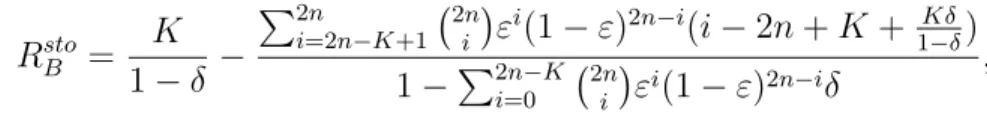
Profits for a seller with capacity constraint K ≤n are
πcsto(K) = 2n X
j=0
min{j, K}Qsto(j)
+βδ
" 2n X
j=K
QstoG (j) K 1−δ +
K−1
X
j=0
QstoG (j)
" P2n i=1
2n i
εi(1−ε)2n−i(min{i, K}+ Kδ
1−δ)
1−(1−ε)2nδ
##
+(1−β)δ
" 2n X
j=K
QstoB (j) K 1−δ −
2n X
j=K
QstoB (j)
" P2n
i=2n−K+1 2n
i
εi(1−ε)2n−i(i−2n+K+ Kδ
1−δ)
1−P2n−K i=0
2n i
εi(1−ε)2n−iδ
##
.
(28)
These profit functions resemble those in the deterministic setting, except incorrect cascades
are now eventually corrected, regardless of whether the seller is unconstrained. Thus, unlike in
our deterministic setting, the logic of Smith and Sørensen (2000) holds here, in the sense that
unboundedly informative signals generate efficient learning in the long run. Incorrect negative
cascades are always corrected as soon as a single informed consumer arrives, and the same
applies for incorrect positive cascades if the seller is unconstrained. For a constrained seller
experiencing an incorrect positive cascade, at least 2n−K+ 1 informed consumers must arrive
in the same period and prevent a sell-out, in order for the state to be revealed.
Theorem 3. For any n >1, K ≤n and δ >
q
2n−K
2n , there are (α, β, ε)∈(1/2,1)×(0,1/2)×
(0,1) and r > 0 for which the seller can increase its profits above the unconstrained level by
restricting capacity to K.
Notice that Theorem 3 holds for some ε, while Theorem 2 holds for all m ≤ n. In the
deterministic setting, an appropriate capacity constraint could stop all further learning after
a sell-out. In the stochastic setting, an incorrect positive cascade really only pays off if the
probability of having many informed consumers is sufficiently low. That being said, the
quali-tative message is similar across the two settings: incorrect positive cascades are more difficult
to reverse if the number of informed consumers is small relative to capacity.
Although incorrect positive cascades are eventually corrected in the stochastic setting, this