Distribution of Diffusion Measures from a Local Mean-Square Displacement Analysis

Distributions of diffusion measures from a local mean-square displacement analysis

1_{Max-Planck Institut f¨ur Physik komplexer Systeme, N¨othnitzer Str. 38, 01187 Dresden, Germany}

2_{Department of Molecular, Cellular and Developmental Biology, Yale University, New Haven, Connecticut 06520, USA}

3_{Faculty of Physics, Center for NanoScience (CeNS), Ludwig-Maximilians-Universit¨at, Geschwister-Scholl-Platz 1, 80539 Munich, Germany} 4_{Bernstein Center for Computational Neuroscience Berlin, Institute of Physics, Humboldt University Berlin, Germany}

(Received 17 April 2012; published 31 August 2012)

In cell biology, time-resolved fluctuation analysis of tracer particles has recently gained great importance. One such method is the local mean-square displacement (MSD) analysis, which provides an estimate of two parameters as functions of time: the exponent of growth of the MSD and the diffusion coefficient. Here, we study the joint and marginal distributions of these parameters for Brownian motion with Gaussian velocity fluctuations, including the cases of vanishing correlations (overdamped Brownian motion) and of a finite negative velocity correlation (as observed in intracellular motion). Numerically, we demonstrate that a small number of MSD points is optimal for the estimation of the diffusion measures. Motivated by this observation, we derive an analytic approximation for the joint and marginal probability densities of the exponent and diffusion coefficient for the special case of two MSD points. These analytical results show good agreement with numerical simulations for sufficiently large window sizes. Our results might promote better statistical analysis of intracellular motility. DOI:10.1103/PhysRevE.86.021926 PACS number(s): 87.10.Mn, 02.50.Fz, 05.40.Jc

I. INTRODUCTION

The analysis of single-particle-tracking experiments is im-portant to reveal valuable information about intracellular trans-port processes and the complex dynamics of the cytoskeleton. Here, mean-square displacement (MSD) is often used to char-acterize intracellular transport phenomena. Organelles inside eukaryotic cells are transported in two ways (two motility modes): (i) pulled by molecular motors along intracellular filaments and (if not bound to a filament) (ii) pushed around by cytoskeletal components. Recent experimental [1,2] and theoretical papers [3] suggest that intracellular transport can be described as a combination of free (sub)diffusion and phases of active transport; for a more detailed picture, see the recent review in Ref. [4]. In most other cell types, tracer particles (comparable in size to organelles) switch stochastically between the two motility modes on a subsecond time scale, possibly optimized for the transport task at hand [3]. Such switchings cannot be resolved by a standard global MSD analysis, which extends over a time scale of seconds or longer. Recently, a novel technique called the local MSD analysis has been introduced [1,2]. Here, the MSD is measured over a comparatively small averaging time window, and the resulting MSD curve is fitted to a power law,

R2_∼tα

(1)

(details of the fitting procedure are discussed below), and the parameters of the fit are related to the diffusion coefficient and the exponent of MSD growth, respectively. In particular, the value ofαdefines the type of motion [5,6]: Forαsignificantly below 1, the particle performs subdiffusion, whereas,αgreater than 1 implies superdiffusion with the limiting ballistic case ofα=2.

The values of diffusion coefficient and exponent are assigned to a reference point (preferably the midpoint)

*_{[email protected]}

of the averaging time window; by sliding the window over the trajectory, one obtains (temporally) local information on the diffusive or transport behavior. Using the time series of the exponent α, one can distinguish typical phases of intracellular motion: phases of subdiffusion and phases of directed transport.

In general, even if the vesicle or bead is restricted to perform only one kind of motion, subdiffusion, for instance, the parameters resulting from the local MSD algorithm will be statistically distributed. Put differently, because we use a temporal finite-size average of the trajectories, the resulting time series for the diffusion coefficient and the exponent are still stochastic. The probability densities of these exponents of growth and of the diffusion coefficient (related to the prefactor of the fitting lawA) will be shaped not only by the properties of the cytoplasm, but also by the MSD algorithm itself. When ex-ploring the properties of the cytoplasm, it is certainly desirable to entangle and to separate these two factors. A good starting point in this regard seems to be the calculation of the statistics for model systems, such as a simple Brownian motion. In a recent paper, we showed that a simple model with correlated Gaussian velocity fluctuations could reproduce the statistics of the MSD parameters of experimental data on intracellular bead motion [7]. Here, we explore this model theoretically and derive approximate expressions for the probability densities of the motion parameters. More specifically, we calculate the joint and marginal densities for the MSD exponent and effective diffusion coefficient. We start with the comparatively simple case of an overdamped Brownian motion (uncorrelated Gaussian velocity fluctuations) and then derive formulas for the more interesting case of a correlated Gaussian velocity leading to transient subdiffusion. For the latter case, we also compare the local MSD analysis to the characteristics of subdiffusion as seen in the long-time MSD average. Our results may contribute to a proper interpretation of the local MSD analysis as it is used by experimental groups.

model: a random motion with Gaussian velocity fluctuations, the correlation function of which is given. We discuss results for this model for two specific choices of the correlation function: (i) uncorrelated velocity noise, corresponding to an overdamped Brownian motion and (ii) a negative exponentially decaying correlation [antipersistent motion (AP)] similar to that found in experiments on intracellular motion. We derive and compare approximation formulas for the case of two MSD points to numerical simulations. We also explore using numerical simulations, the more involved case of more than two MSD points and discuss our results in comparison to the exact MSD obtained by a long-time average. The paper concludes with a summary and discussion of our findings. Details of the analytical derivations are discussed in the Appendix.

II. LOCAL MSD ALGORITHM

The conventional method of analyzing experimentally recorded trajectories is based on estimates of the MSD. For a trajectory of time lengthT, the MSD is approximately given by

R2 t(τ)=

1

T −τ T−τ

0

ds[R(t+s+τ)−R(t+s)]2. (2)

For the case of Brownian motion, the time average shown in Eq.(2) can be replaced by an ensemble average taken over a large number of trajectories (this is not necessarily true for subdiffusive motion as has been observed in a number of recent papers [8–10]). More important for the current paper is that, for a finite time window, the resulting estimate of the MSD is still noisy. How these finite-size fluctuations affect the fluctuations of the motion parameters is the topic of our paper.

For a discretized trajectory x_il =xl(t+i t) with i=

0, . . . ,M (sampling step t) and l=1, . . . ,d (where d is the number of spatial dimensions), this average of overlapping segments reads

R2

t(τ =k t)= 1

M−k+1 M−k+1

i₌1 d

l₌1

x_il_+k−1−x_il₋₁2.

(3)

A local MSD is the same as Eq.(2), but the average is taken over a small local time windowT for different values of the time incrementτ. The resulting data are then reduced to pure numbers by dividing distances by a length scale, e.g., simply the length unit=1μm [for our choice ofin our numerical examples, see below after Eq. (5)], and time by a reference time τ0. The local MSD at mτ different values (number of MSD points) ofτ is then fitted to a power law,

R2 t(τ)

2 =A

τ τ₀

α

. (4)

The exponentαcarries information about the motion type [5]:

α <1 implies subdiffusion, α≈1 implies normal diffusion (Brownian motion), α >1 implies superdiffusion, and α≈

2 implies ballistic motion. The prefactor Ahas no physical dimension. The diffusion coefficient is directly proportional to the prefactorA. More specifically, if we set the time lagτ

equal to the reference timeτ0, we obtain

D= R

2 t(τ0) 2dτ0

= A2

2dτ0

=AD₀, (5)

where d is the number of spatial dimensions and D₀= 2/(2dτ0) is a parameter that carries the physical dimension of a diffusion coefficient and is set by our time and length scales. In the examples inspected below, we work with nondimensional units and setandtsuch that the numerical value ofD₀=1. We also set the reference timeτ₀equal to the maximal lag time (i.e.,τ0=mτt, wheremτ is the number of MSD points). For general applicability of our formulas, however, we keep D0, , τ0, and t in all formulas as free parameters.

The fit to the power law is performed by linear regression in a double logarithmic plot of the data. To this end, themτ pairs,

ln(k/mτ),ln

R2t(k t)/2 , k=1, . . . ,mτ (6)

are fitted to

f(ln(k/mτ))=lnA+αln(k/mτ), (7)

by the well-known formulas of linear regression [11] yielding the slope α and the prefactor lnA related to the diffusion coefficient byA=D/D0according to Eq.(5),

α=

kln

R2

t(k t)/2

ln(k/mτ)−_m1_τ

k,jln

R2

t(j t)/2

ln(k/mτ)

k(ln(k/mτ))2−m1τ kln(k/mτ)

2 , (8)

lnA= 1 mτ

k

lnR2t(k t)/2

−αln

k mτ

. (9)

Here, the indexk(and alsoj) runs fromk=1, . . . ,mτ. Sliding the time window T =M t over the entire trajectory [cf. Fig. 1(a)], the motion parameters D(t) and α(t) can be extracted as functions of time. Because one uses a small time

0 0.5 1

t

0 1 2

α

0 0.5 1

t

0 2 4

D

=

A / 2

τ 0

0 0.5 1

t

0 2 4 6

x

(

t

)

-1 -0.5 0

log₁₀(kΔt/τ₀) -3

-2 -1

log

10

(

Δ

R / l

)

MSD points

Fit: log A + αlog (kΔt/τ )

(a)

(c) (b)

2

2

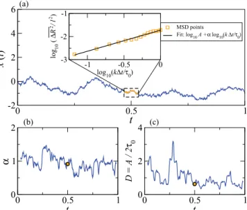
FIG. 1. (Color online) Illustration of the local MSD algorithm. (a) Trajectory of a Brownian particle is analyzed locally in a time window ofM points (trajectory inside the dotted rectangle): The squared displacement formτ points is averaged over theseMpoints and is fit by a linear relationship in log-log space [see inset of (a)]. The resulting slope (exponent) and intercept (proportional to the diffusion coefficient) are assigned to the midpoint of the window. By sliding the window over the trajectory, in this way, we obtain a time series of the exponent (b) and the diffusion coefficient (c). The circular dots in each (b) and (c) are the values obtained in (a). The trajectory is obtained using Eq. (10) for overdamped Brownian motion. Parameters used here are as follows:mτ =15, M=60, t=10−3_, andD=kBT /γ =1.

The local-MSD algorithm has two parameters: M, the number of points in the time window andmτ, the number of values ofτused in the power law fit. HowMandmτinfluence the statistics of the estimated values ofαandDis a question of foremost interest in our paper. For simple illustrations of our results, in this paper, we will exclusively consider the one-dimensional case. For the model introduced in the next section, the generalization of our analytical approximations to the multidimensional case is straightforward.

III. MODEL WITH PRESCRIBED VELOCITY FLUCTUATIONS

In our model, the dynamics of the displacement of a vesicle or bead is described by

˙

x =v, (10)

where the velocity is assumed to be a stationary Gaussian stochastic process with vanishing mean value and correlation function,

v(t)v(t+τ) =C(τ), (11)

where·denotes the ensemble average.

In discrete time [xi =x(i t) with time step t], a trajectory (sample path) of the process can be simulated by the simple map,

xi+1=xi+vit. (12)

The correlation of the incrementsvi=[xi+1−xi]/tcan be related to the continuous correlation functionC(τ) as follows:

Ck = vi+kvi

=

t

0

dτ[C((k−1)t+τ)

+C((k+1)t−τ)] τ

(t)2. (13) For a sufficiently small time step (within which the correlation function does not change much) but largek withT =k t, the integrand can be approximated by 2C(T)τ/(t)2_{, and one} obtains the intuitive result,

Ck≈C(k t), t C(k t)/C˙(k t). (14)

In this limit, the discrete correlation agrees with the continuous correlation.

Traditionally, the time-continuous Eq.(10)with the correla-tion funccorrela-tion Eq.(11)is regarded as the model to be considered. Equivalently, we can, however, consider the map Eq.(12)and the discrete correlation function as our starting point. This is practical in two respects. First, to simulate a sample path of the system, we need a temporal discretization in any case. Second, the velocity correlation might be obtainable from experimental data only in a discretized version, so typically, we know Ck but not C(τ). In this paper, we will solely use the discrete version as our starting point. We now discuss how to simulate sample paths and introduce two simple variants that are used as numerical examples.

We assumed above that the noise has Gaussian statistics. Under these circumstances, the velocity process can be simulated as an autoregressive (AR) process [11] as follows:

vi = p

k₌1

dkvi−k+gi, (15)

where gi are uncorrelated Gaussian random numbers with mean zero and variance σ2

g. The coefficients dk of this AR process can be obtained from the experimental incremental correlation function by the formula,

d=P−1C/σ_v2, (16)

where d=(d₁,d₂, . . . ,dp) is the vector of unknown coef-ficients, C=(C₁,C₂, . . . ,Cp) is the vector of the discrete correlation function, and the matrixPis given by

P=

⎡ ⎢ ⎢ ⎢ ⎢ ⎣

1 ρ1 ρ2 · · · ρp₋1

ρ1 1 ρ1 · · · ρp−2

..

. ... ... · · · ...

ρp−1 ρp−2 ρp−3 · · · 1

⎤ ⎥ ⎥ ⎥ ⎥

⎦, (17)

where

ρk =Ck/C0 (18)

is the normalized correlation coefficient. The variance can be found from

σ_g2 =C₀−

p

k₌1

dkCk. (19)

We will consider two simple special cases in this paper. First, for uncorrelated velocity fluctuations, the map Eq.(12)is just the discrete version of overdamped Brownian motion [12],

CWN(τ)=2kBT

γ δ(τ) → C

WN k =2

kBT

γ tδk,0 (20)

[WN stands for white noise]. Here, kB is the Boltzmann constant, T is temperature, and γ is the Stokes friction coefficient. In this case, all the coefficients dk in Eq. (15) are zero, and the variance in the driving fluctuations reads

v2_i=g2_i=C₀=2kBT

γ t. (21)

For the white-noise case, the mean-square displacement is given by a pure diffusive law,

x_k2:= (xi₊k−xi)2 =k(t)2C0=k t

kBT

γ . (22)

In our second example, we will consider a finite discrete correlation that is negative at all finite lags and decays exponentially,

C_kAP=(C0−C1e1/kd)δk,0+C1e−(k−1)/kd, (23) where, with C0 >0 and C1 <0, the correlations are the characteristics of an anti-persistent (AP) type of motion. Such

correlations have been recently observed experimentally for different kinds of organelles and particles [7,13]. We note that, on physical grounds,C1 cannot take arbitrary values but has to obey

|C1|(e1C0)/2, (24)

wheree1=(1−e−1/kd). The exact mean-square displacement for this motion can be calculated [14] and reads

x_k2=t2

k

C0+ 2C1

e1

−2C1

e2 1

(1−e−k/kd₎

. (25)

Interestingly, the MSD grows linearly with time at small times,

x_k2

smallk ≈k t 2

C0+

2C₁(e₁−1/kd)

e2₁

, (26)

and asymptotically at large times [as long as in Eq.(24)the equality does not hold],

x_k2_largek≈k t2

C0+ 2C1

e₁

. (27)

In between these asymptotics, there exists a transition region characterized by a subdiffusive behavior [cf. Fig. 2(f)].

-0.1 0 0.1

v

Δ

t

0 3 6 9

P

(

v

Δ

t

)

-1 -0.5 0 0.5 1

v

Δ

t

0 0.5 1

P

(

v

Δ

t)

5 10 15 20 25 30

k

-0.1 0 0.1

ρ

5 10 15 20 25 30

k

-0.1 0 0.1

ρ

-3 -2 -1 0 1

log

(k

Δ

t)

-3 -1.5 0 1.5

log

10

〈Δ

x

2

(

k

Δ

t

)

〉

-1 0 1 2

log

(k

Δ

t)

-1.5 0 1.5

log

10

〈Δ

x

2

(

k

Δ

t

)

〉

(a) (b)

(d) (c)

(f) (e)

Assumingkd 1, the condition for this range reads

ε C0

|C₁| k

1/e₁

ε[C₀e₁/(2C₁)−1], (28)

whereεis the relative deviation of the respective asymptotic expression from the exact result, e.g., for the small-k asymp-totics,

ε= x

2

smallk− x2

x2 1. (29)

Simple Brownian motion is a special case with C1=0 in which the two asymptotic regimes coincide and there is no transition region of subdiffusion. For finite negative correlations (C1<0), the region of subdiffusion is not entirely determined by the correlation time of the incrementskdt, but also by the strength of the negative correlations, which is set by 2C1/(e1C0).

We emphasize that we consider a situation in which the full mean-square displacement is not considered because we have only a short (temporally local) sample of the particle’s trajectory. Below, in Sec.V, we will compare the statistics to that of the full mean-square displacement curve.

IV. THE STATISTICS OF THE LOCAL MSD PARAMETERS We know that the increments (estimates of the instanta-neous velocity) are Gaussian distributed and that their linear correlation is given by the functionCk. The calculation of the statistics of a finite-size MSD (the square of a sum of correlated Gaussian variables or, more generally, a quadratic form) is a classical problem in the theory of stochastic processes (see Ref. [15] and references therein). However, what enters into the local MSD algorithm, in general, are sums over logarithms of such squared sums of Gaussian increments, i.e., a strongly nonlinear function of the simple Gaussian variables that we start with. Apart from special cases, it is difficult to calculate statistical distributions of such nonlinear functions of sums of Gaussians, and so, we are forced to use reasonable approximations. One such approximation for the case of only two MSD points but a large number of averaging pointsMwill result in a Gaussian distribution ofαand ln(D/D₀) [where, according to Eq.(5),A=D/D₀] because, in forming these numbers, we effectively add up many sufficiently independent random numbers, i.e., in the limit of large M, the central limit theorem applies. Under the assumption of a Gaussian distribution, it remains to calculate mean values and second-order moments (variances and covariances) of ln(D/D₀) and

α. In the Appendix, this is performed in the general case of a correlated Gaussian velocity noise with discrete correlation functionCk. We obtain

α =1+ln(1+ρ1)

ln 2 , ln(D/D0) =ln

(C0+C1)t 2D0

,

σ_α2 = s1+ρ

2

1g2Ms2−2ρ1gMs3 [(C0+C1)(M−1) ln 2]2

,

σ2

ln(D/D0 ) =

s₁+s₂+2s₃

[(C₀+C₁)(M−1)]2 −1,

σ_αln(D/D

0 ) =

s1−ρ1gMs2+(1−ρ1gM)s3 [(C0+C1)(M−1)]2ln 2

, (30)

wheregM =1−1/Mand we have further abbreviated

s1 =M

C₀2+MC₁2gM

+2

M₋2

i₌1

(M−i−1)C_i2+Ci−1Ci+1

,

s2 =M(M+1)C02gM+4MgM M₋2

i₌1

(M−i−1)C_i2, (31)

s3 =M(M−2)C0C1gM

+2

M₋2

i=1

[2(M−i)−1]CM₋i₋1CM₋i.

Using these values, the Gaussian approximations of the joint probability density and the marginal densities are com-pletely determined. They are given by

P(α)= 1 2π σ2

α exp

−(α− α)2

2σ2 α

, (32)

P(D)= (D0/D) 2π σ2

ln(D/D0 )

exp

−[ln (D/D0)− ln(D/D0)]2 2σ2

ln(D/D_{0 )}

,

(33)

P(D,α)=

√

4ab−c2 2(D/D0)π exp

−a(ln (D/D0)− ln(D/D0))2

−b(α− α)2−c(α− α)

×(ln (D/D0)− ln(D/D0)) . (34)

The coefficients (a,b,c) appearing in Eq.(34)are derived using the first and second moments. In this paper, we plot ˆP(ln(D/D₀),α) instead of P(D,α) because the former function is more symmetric with respect to its arguments,

ˆ

P(ln(D/D0),α)=

√

4ab−c2

2π exp

−a(ln(D/D0)

− ln(D/D0))2−b(α− α)2

−c(α− α)(ln(D/D0)− ln(D/D0)) .

(35)

In the following section, we discuss these formulas and com-pare them to numerical simulations for the two special cases (overdamped Brownian motion and antipersistent motion).

A. Results for an overdamped Brownian motion The general formulas derived above reduce to quite simple expressions if the velocity is uncorrelated over a finite lag time (Ck =0 fork >0),

α =1, ln(D/D0) =ln

kBT /γ

D₀

, (36)

σ_α2 = 1

(M−1)(ln 2)2, σ 2

ln(D/D0 ) =

3

(M−1), (37)

σ_αln(D/D

0 ) =

1

0 0.5 1 1.5 2

α

0 1 2 3

P

(

α

)

M = 10 M = 20 M = 100 Theory

0 0.5 1 1.5 2 2.5

D

0 1 2 3

P

(

D

)

(a)

(b)

FIG. 3. (Color online) Marginal distributions of (a)αand (b)D resulting from the local MSD algorithm for overdamped Brownian motion; data sets differ by the size of the rolling window as indicated. The number of local MSD points for all simulation data (symbols) is mτ =2; theoretical approximations Eqs.(32)and(33)are shown by lines.

The coefficients for the joint probability distribution are given by

a= (M−1)

4 , b=

3(M−1) 4 (ln 2)

2_{, c= −}(M−1) 2 ln 2.

(39)

In the following, we setD=kBT /γ =1 in our simulations (this completely determines the physics of the process) and vary only the parameters of the local MSD algorithm. The time step for integration is taken ast =10−3. The analytical approximations for the first and second moments can be obtained from Eq.(30).

In Fig.3, we compare the marginal distributions of α (a normal distribution) and D (a lognormal distribution) with numerical simulations. The quality of our approximation depends strongly on the number of points in the sliding window. Whereas, forM=10, there is a finite discrepancy between simulation and theory, the agreement forM=100 is very good. The values ofαare equally distributed around the expected mean of 1, and the distribution of the estimated

D is much more skewed, in particular, for smaller values ofM.

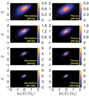
In Fig.4, we show the joint probability density ofα and ln(D/D₀) for simulation data and analytical approximations side by side. According to our analytical calculation, this should be a two-dimensional Gaussian (corresponding to ellipsoid contour lines) with a clear correlation between the variables. The correlation is indeed evident for all values of

M; the simulation data for M=10, however, do not show the symmetry of a Gaussian (contour lines are not perfect ellipsoids). For larger M, the probability is confined to a

α

α

α

Simulation

(M=10) Theory(M=10)

Simulation

(M=20) Theory(M=20)

Simulation

(M=60) Theory(M=60)

α

Simulation

(M=100) (M=100)Theory

ln(D/D0) ln(D/D0)

FIG. 4. (Color online) Joint distribution of α and lnA for an overdamped Brownian motion and two MSD points (mτ=2): left column: simulation results compared to right column: theory Eq.(34) for various numbers of points of the rolling window as indicated.

much smaller range of α and ln(D/D0) but also becomes more symmetrically distributed.

Why do the two parameters show such a strong positive correlation? This could have the following reason. Consider all the points on the straight line (the true MSD curve in a double logarithmic plot) and then add an independent noise of equal amplitude to each point along the line. The intercept (corresponding to the diffusion coefficient) is given by the right-most point in the MSD curve (the MSD value at maximum lag time), and the exponent is given by the slope of the line. It is not hard to estimate that the resulting correlation between slope and intercept is positive. The value of this positive correlation, however, is much smaller than the correlation evident in the joint density. The strong positive correlation relies on the fact that the noise along the MSD curve is positively correlated, leading to an additional positive correlation in additive constant and slope.

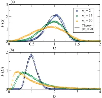
Next, we discuss the marginal distributions as a function of the MSD points (Fig.5); the number of points in the sliding time window is set toM=60. One interesting question here is whether the variability of the estimated parameters decreases or increases if we take more than two MSD points into account. For once, every estimation of the MSD slope should become better by having more points. On the other hand, the points that we add are more noisy than the first two points, so our estimate should become more noisy. As apparent from the simulation results shown in Fig.5, the latter effect dominates, and thus, the distributions (of both αand diffusion coefficientD) for larger numbers of MSD points are generally more variable than those for two MSD points.

0 0.5 1 1.5 2

α

0 1 2 3

P

(

α

)

m_τ = 2 m_τ = 15 m_τ = 30 Theory (m_τ = 2)

0 1 2 3 4

D

0 1 2

P

(

D

)

(a)

(b)

FIG. 5. (Color online) Marginal distributions of (a)αand (b)D resulting from the local MSD algorithm for overdamped Brownian motion. Data sets differ by the number of MSD pointsmτas indicated but have the same window size ofM=60 points.

discussed in Fig. 6 as functions of (a) and (b) the window sizeMand (c) and (d) the number of MSD points. Looking at meanα, we observe an underestimation of the true exponent of 1 for both smallM and a large number of MSD points. At the same time, the variance in the α distribution drops

strongly with M. Furthermore, it undergoes a minimum if the number of MSD points is varied; this shallow minimum is attained at mτ =4, and the minimum’s value does not differ much from what we observe for two MSD points (the analytically tractable case). These observations indicate that a few tens of points in the rolling window and a small number of MSD points (preferably: 2) are recommendable for a reliable estimation of an overdamped Brownian motion’s MSD exponent.

The results are for the mean and standard deviation of the diffusion coefficient’s estimate point, although not as strongly, in the same direction. The mean of the diffusion coefficient does neither depend strongly onMnor on the number of MSD points. The standard deviation, however, drops strongly with

M and increases with the number of MSD points. So, also for a reliable estimate of the diffusion coefficient, the case of largeMand minimal number (=2) of MSD points seems to be optimal. This highlights the importance of the case that we are able to treat analytically.

B. Results for an antipersistent motion

Now, we tackle the more involved but interesting extension of a correlated velocity process with correlation function Eq. (23). Here, the increments are negatively correlated in qualitative accordance with recent experimental findings [7,13]. Our general result can be simplified for this specific correlation function because the parameters s1, s2, and s3, which determine the variances and covariances ofα, can be

0 0.6 1.2

〈α〉

Theory (2 MSD pts)

0.95 1 1.05

〈

D

〉

〈

D

〉

1 10 100

M

0.1 1

σ

1 10 100

M

0.1 1

σ

D/D

0

)

0 0.5 1

〈α〉

Simulation (M=60)

0.9 1 1.1

0 10 20 30 40 50

m

0.4

σ

0 10 20 30 40 50

m

0.5 1

σ

D/D

0

)

(a) (b)

(d) (c)

recast into the following forms:

s₁=MC2₀+(M2+3M−2)C₁2+2(M−1)C₀C₁e−1/kd+4C

2

1[e−2(M−2)/kd+(M−2)e2/kd−(M−1)]

(e2/kd−₁₎2 , (40)

s2 =M(M+2)C02+ 4C2

1e2/kd[e−2(M−1)/kd+(M−1)e2/kd−M]

(e2/kd −1)2 , (41)

s3 =(M2+3M−2)C0C1+2C12e 3/kd[e

−2(M−1)/kd+_e−2M/kd+₍₁−_2M)e−2/kd +_(2M−_3)]

(e2/kd−1)2 . (42)

Parameters of the correlation function are chosen as follows:

C0=0.1/t2, C1= −0.01/t2, andkd =4, yielding incre-ment correlations similar to those observed experiincre-mentally in Ref. [7]. We choose the time stept =45×10−3 _{such that} the mean diffusion coefficient formτ =2 is unity.

In Fig.7, we show marginal distributions ofαandD for various sizesMof the rolling window. As in the white-noise case, the agreement with our theory becomes better for increasingM and is remarkably good for a time window of aboutM=100 points. In general and as expected, both kinds of distributions become less variable when M is increased. However, in contrast to the case of overdamped Brownian motion (shown in Fig.3), the mean value ofαalso depends strongly on the size of the window. In particular, the mean value for allMshown here is consistently lower than 1. This is an effect of the negative increment correlations.

For the joint distribution, we observe effects very similar to the white-noise case (see Fig. 8). The parameters α and ln(D/D0) are positively correlated for the same reasons as discussed in the previous subsection. Furthermore, the joint density for smallMshows some asymmetry that is inconsistent with our Gaussian approximation. This asymmetry becomes, however, less pronounced for increasing window sizeM.

0 0.5 1 1.5 2

α

0 1 2 3

P

(

α

)

M = 10 M = 20 M = 100 Theory

0 0.5 1 1.5 2 2.5

D 0

1 2 3

P

(

D

)

(a)

(b)

FIG. 7. (Color online) The marginal distributions of the MSD exponentαand the diffusion coefficientDfor negatively correlated increments (antipersistent motion). Various sizes of the rolling time window are indicated; simulation and analytical results are shown by symbols and lines, respectively.

We turn again to the marginal distributions, inspecting now, by numerical simulation, the case of more than two MSD points (see Fig.9). Clearly, as in the white-noise case, more than two MSD points increase the variability of the distributions. In marked contrast to the white-noise case, the number of MSD points also has a drastic effect on the estimated mean exponent of MSD growth and on the mean diffusion coefficient. Both decay strongly with increasing numbers of MSD points.

This aspect of the data becomes clearly visible in Fig.10 where again, we show the mean values and standard deviations ofαandDas functions of window sizeMand number of MSD points. The behavior of the standard deviation is similar to the white-noise case (cf. Fig. 6). However, the mean exponent’s decay with the number of MSD points as well as its saturation for increasing M at a value below 1 is a clear consequence of the negative increment correlations and very different from what we observed for the overdamped Brownian motion.

The decrease in the mean exponent with an increasing number of MSD points is in line with the behavior of the exact MSD as a function of lag time: With increasingmτ, we take more points from the subdiffusive transition region of the MSD curve into account and—being far away from the long-time asymptotic diffusive limit—this results in a drop in

α

α

α

Simulation (M=10)

Theory (M=10)

Simulation (M=20)

Theory (M=20)

Simulation (M=60)

Theory (M=60)

α

Simulation (M=100)

Theory (M=100)

ln(D/D0) ln(D/D0)

0 0.5 1 1.5 2

α

0 1 2 3

P

(

α

)

m_τ = 2 m_τ = 15 m_τ = 30 Theory (m_τ = 2)

0 0.5 1 1.5 2

D

0 1 2 3 4

P

(

D

)

(a)

(b)

FIG. 9. (Color online) The marginal distributions of the MSD exponentαand the diffusion coefficientDfor negatively correlated increments (antipersistent motion). Here, the number of MSD points is varied as indicated; theory is only plotted formτ =2.

the mean exponent as estimated by the local MSD analysis. With respect to this behavior, the question about the optimal

mτ is more complicated. From the statistical point of view, it is certainly recommendable, as in the case of overdamped Brownian motion, to choose a rather small number of MSD points. In order to catch the subdiffusive behavior, however,

one would rather favor a larger value of mτ that yields a mean exponent more distinctly from 1. Looking at Fig.10(c), a value with much smaller α but still comparably small fluctuations would be given at about a quarter of M, here,

mτ =15=M/4. This is also the value that has been used in different applications of the MSD analysis [1,7].

V. SUBDIFFUSION ON LONGER TIME SCALES FORM→ ∞

So far, we have focused on small (local) time windows for the determination of the motion parametersαandD. This is relevant in the situation in which these parameters change over time as is the case, e.g., for the intracellular motion of vesicles. It is, however, instructive, to compare our results of the local MSD analysis to the exact MSD curve and its derivative for a long-time window (M→ ∞). We focus here solely on the exponentαin order to obtain some intuition for time scales for which this statistics reflects subdiffusional behavior. We reiterate that the situation considered in this section (M→ ∞) is not a common one in which one would apply the local MSD algorithm.

In the limitM→ ∞, the finite-size estimate of the MSD used in Eq.(8)becomes an exact average (x2_{→ x}2_as

M→ ∞). In this limit, the value ofαapproaches the noiseless quantity,

α_∞= mτ

k=1ln

x_k2ln_mk

τ

− 1

mτ mτ

k,j=1ln

x2_jln_mk

τ mτ

k₌1

ln_mk

τ

2₋ 1 mτ

mτ

k,j₌1ln

_k

mτ

2 .

(43)

0 0.5 1

〈α〉

Theory (2 MSD pts)

0.9 1 1.1

〈

D

〉

1 10 100

M

1

σ

1 10 100

M

1

σ

D/D

0

)

0 0.5 1

〈α〉

Simulation (M = 60)

0 0.5 1

〈

D

〉

0 10 20 30 40 50

m

0.1 0.2

σ

0 10 20 30 40 50

m

0.2 0.4 0.6

σ

D/D

0

)

(a) (b)

(d) (c)

For the white-noise case, inserting the exact MSD according to Eq.(22)into Eq.(43)yieldsα_∞=1 as can be expected. Hence, the deviations that are seen in Fig.6(c)at large values ofmτare due to the finite sample estimation of the MSDxk2, i.e., the deviations become severe ifmτ does not differ much fromM, here, forM=60, this is true formτ 20. Before we discussα_∞for the correlated velocity process, we would like to recall the behavior of the exact MSD for this case.

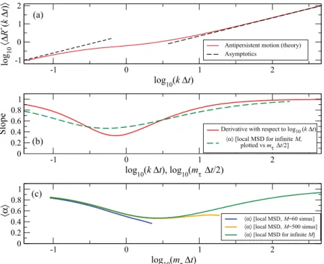
In Fig. 11(a), we show the exact MSD according to Eq. (25) [this was already shown in Fig. 2(f)] together with the asymptotic results (dashed lines) for small and largek’s, i.e., Eqs.(26)and(27), respectively. The range of subdiffusion is in agreement with Eq.(28)roughly given by log₁₀k t ∈(−1.3,1.3) (here, we usedε=0.1) and coincides with the range for which the slope of the MSD curve [see Fig. 11(b), solid line] is significantly smaller than 1. The latter derivative attains a minimum and, in this way, indicates a most subdiffusive behavior that is determined by the temporal extension as well as by the strength of the negative correlations.

The functionα_∞for the correlated velocity process can be obtained by inserting the exact MSD Eq.(25)into Eq.(43). As shown in Fig.11(c)by the green line, it also attains a minimum, although at a value ofmτt that is larger than the timek t at which the slope of the exact MSD becomes minimal. This is not surprising because Eq.(43)takes into accountallMSD valuesup to the maximal lag mτ (more specifically, it is a weighted sum of these values). In contrast, the derivative in the MSD-log-log plot takes into account only local features of the MSD curve. To better compareαto the local slope of the MSD curve [solid line in Fig.11(b)], we can associate

α_∞with the mean time scale of the whole window, which we may take approximately ashalfthe maximum time. If we plot theα_∞against log₁₀(mτt /2) [dashed line in Fig.11(b)], we obtain a curve with a minimum close to that of the derivative of the MSD. It is important that the time scale of maximal subdiffusion can be recovered by the algorithm in this way, provided the time window is long enough to cover the time range of sublinear MSD growth.

For finite values ofM, we illustrate the finite-size noise effect of the numerically measuredαforM=60 (blue line) andM=500 (orange line). Both curves follow the exact mean value until they start deviating due to the effect of the finite-size estimation of the MSD. This illustrates that one cannot trust values ofαthat are determined for a number of MSD points only marginally smaller than the averaging window.

The results of this section also illustrate the simple point that we cannot extract subdiffusive behavior at time scales that are equal to or larger than the size of the averaging window. Still, the local MSD analysis already can show, for comparable small time windows, that the motion is qualitatively distinct from overdamped Brownian motion.

VI. SUMMARY AND CONCLUSIONS

In this paper, we have calculated the statistics of a local MSD algorithm in the special limit of two MSD points and a large averaging window. Our results for the joint and marginal probability densities revealed good agreement. Moreover,

further numerical simulations for larger numbers of MSD points indicated that the limit case we studied was important, giving, for our simple examples, the most reliable and unbiased mean values and the smallest variance in the distributions of MSD exponent and diffusion coefficient. However, we also discussed that a larger number of MSD points might be favorable to show a more distinct subdiffusive behavior of the motion.

In this paper, we also demonstrated how negative correla-tions between increments of the motion (antipersistent motion) yields subdiffusive behavior (α <1) on the small time scale of the local MSD algorithm. In the aforementioned special case of two MSD points, we could characterize this apparent subdiffusion analytically.

The case of antipersistent motion presented here shows transient subdiffusive behavior: At small and long time scales, the motion is diffusive. This is in contrast to persistent subdiffusion that has been observed previously in single cell tracking experiments with motion statistics similar to those of either a continuous time random walk (CTRW) [16,17] or a fractional Brownian motion (FBM) [13,17–19]. Identifying the underlying mechanism that leads to anomalous diffusion (CTRW or FBM) is an important open question and has been raised before in several papers wherein new trajectory analysis tools [20–22] were introduced to address this issue. The analysis presented in this paper does not address these questions.

Our results are interesting for applications in biological experiments in two respects. First of all, our results may be used to check the reliability of experimental estimates of the local MSD properties. For instance, one may discuss for which size of the rolling window it is meaningful to talk about subdiffusion once one observes mean exponents below 1. The results for the correlated Gaussian velocity process studied in this paper give orientation regarding this question.

Second, in comparing to the simple limit case of over-damped Brownian motion, experimentalists may distinguish how strongly the local MSD properties are influenced by the nonequilibrium environment of the cell. To this end, one may compare our simple formulas for the marginal densities for two MSD points to the statistics observed experimentally. In one specific example [7], this yielded the insight that the variability of the estimated parameters for intracellular data (motion of a bead internalized by Dictyostelium discoideum cells) is comparable to that obtained for simple Brownian motion, hence, this variability cannot be ascribed to specific biological properties of the cytoplasm in the living cell. Such conclusions may now also be possible for the study of intracellular motion in other cell types, such as neurons, cancer, and immune cells.

-1 0 1 2

log₁₀(kΔt)

-1 0 1 2

log

10

〈Δ

R

2 (k

Δ

t

)

〉

Antipersistent motion (theory) Asymptotics

-1 0 1 2

log

10(kΔt), log10(mτ Δt/2)

0 0.2 0.4 0.6 0.8 1

Slope Derivative with respect to log₁₀ (k Δt)

〈α〉 [local MSD for infinite M, plotted vs m Δt/2]

-1 0 1 2

log₁₀(m_τΔt)

0 0.2 0.4 0.6 0.8 1

〈α〉 _{M=60 simus]}

M=500 simus]

M]

(a)

(b)

(c)

〈α〉 [local MSD, 〈α〉 [local MSD, 〈α〉 [local MSD for infinite

FIG. 11. (Color online) Comparison of the exact MSD, its derivative, and the mean value of α forM→ ∞. (a) Solid line: exact MSD Eq.(25)for the correlated velocity process and its asymptotic limits for small [Eq. (26)] and large times [Eq.(27)]. (b) Derivative of the MSD log-log plot, i.e.,dlog₁₀[x2_{(t)]/d log}

10(t) is compared to the mean value ofαforM→ ∞ plotted vs the logarithm of half the maximal time window log10(mτt /2). (c) Mean value ofαfor various values ofMas indicated vs maximal lag timemτt.

function, relating such a model to the biophysical situation in the cell is still not fully understood (for a notable exception, see the recent Ref. [13]) and is certainly worth further study. Another unexplored venue is what kind of statistics the local-MSD algorithm yields for non-Gaussian velocity fluc-tuations, such as, for instance, in models of active Brownian motion [23] or coupled molecular motors [24], which have obvious significance for intracellular motility [25]. This leaves numerous exciting questions for future investigations.

ACKNOWLEDGMENT

A.N. and B.L. acknowledge support from the Max Planck Society.

APPENDIX: THE STATISTICS OF THE MOTION PARAMETER FOR TWO MSD POINTS (mτ =2) Substituting the expression for the discrete-time trajectory [Eq. (12)but in d dimensions] in the local-MSD algorithm [Eq.(3)], the estimate of the MSD, in terms of the velocity fluctuations, is given by

R2

t(k t)=

t2

(M−k+1) M₋k₊1

i=1 d

l=1

⎛

⎝k

j=1

v_il_+j−1 ⎞ ⎠

2

. (A1)

Dividing by 2 _{and taking the logarithm on both sides,} Eq.(A1)becomes

ln

R2

t(k t)

2

=ln

⎡

⎣ t2/2

M−k+1 M−k+1

i=1 d

l=1

⎛

⎝k

j=1

v_il_+j−1 ⎞ ⎠

2⎤

⎦. (A2)

For the special case ofd =1, Eq.(A2)becomes

ln

xt2(k t)

2

=ln

⎡

⎣ t2/2 M−k+1

M−k+1

i₌1

⎛

⎝k

j₌1

vi+j−1

⎞ ⎠

2⎤

⎦.

(A3)

To determine the intercept lnA and slope α according to Eq.(7), we use themτ pairs [ln(k/mτ),ln(Rt2(k t)/2)] in the formulas of linear regression, yielding Eqs.(8)and(9). The latter equations express the desired quantities in terms of a sum of logarithms of sums of correlated Gaussian variables. In other words, the statistics of ln A=ln(D/D0) andαis determined by highly nonlinear and lengthy functions of the Gaussian velocity fluctuations. It is, thus, generally quite difficult to relate the probability functions of α and D to those of the velocity fluctuations, in particular, if mτ3. However, for the case of two MSD points (mτ =2), approximate analytical expressions for the marginal and joint distributions ofαand

Dcan be derived.

For two MSD pointsmτ =2 andd =1, using Eq.(8), the exponentαis given by

α= 1

ln 2

lnx2

t(2t)/2

−lnx2

t(t)/2 . (A4)

Using Eq.(A3)in Eq.(8), this can be written as

α=1+ 1 ln 2

⎡ ⎣ln

⎛

⎝ t2/2

2(M−1) M−1

i₌1

(vi+vi+1)2

⎞ ⎠

−ln

⎛ ⎝t2/2

M

M

i=1

v_i2 ⎞ ⎠ ⎤

Similarly, using Eq.(A3)in Eq.(9), the diffusion coefficient is given by

β =ln(D/D₀)=ln

⎛

⎝xt2(2t)

2

⎞ ⎠

≡ln 2+ln

⎛

⎝ t2/2

2(M−1) M₋1

i=1

(vi+vi₊1)2

⎞

⎠, (A6)

where we use, in the following,βas a shortcut for the logarithm of the diffusion coefficient. Note that, in the special case

mτ =2, the estimate of the diffusion coefficient (but not that of the exponentα) corresponds to a quadratic form of a Gaussian. For the latter problem, there exist alternative analytical methods to approximate the probability distribution (see, e.g., Ref. [15] and references therein) than presented in the following.

The arguments of the logarithms in Eqs. (A5) and (A6) are finite-size estimates ofC0= vi2andC0+C1(where the latter term wasC1= vivi₊1); deviations from the true mean values are expected to be small, and so, it is reasonable to expand the logarithms around these values, yielding

ln

⎛ ⎝t2/2

M

M

i₌1

v2_i ⎞ ⎠_≈ln

C0t2

2

+

⎛ ⎝C0−1

M

M

i₌1

v_i2−1

⎞

⎠, (A7)

ln

⎛

⎝ t2/2

2(M−1) M₋1

i=1

(vi+vi₊1)2

⎞ ⎠_≈ln

(C0+C1)t2

2

+

⎛

⎝(C0+C1)−1 2(M−1)

M₋1

i=1

(vi+vi₊1)2−1

⎞

⎠. (A8)

Equations (A5) and (A6) are then given as

α=1+ln(1+ρ1)

ln 2 +

(C0+C1)−1 ln 2

⎛

⎝ 1

2(M−1) M₋1

i=1

v_i2+v_i2₊₁+2vivi₊1

−(1+ρ1)

M

M

i=1

v2_i ⎞

⎠, (A9)

β =ln

(C0+C1)t 2D0

+

⎛

⎝(C0+C1)−1 2(M−1)

M−1

i₌1

v_i2+v2_i+1+2vivi+1

⎞_⎠

−1, (A10)

whereρ1 =C1/C0is the correlation coefficient at lag 1. Using the fact that

M−1

i₌1 vi2/(M−1) =C0and

M−1

i₌1 vivi₊1/(M− 1) =C1, we obtainαandβfrom Eqs.(A9)and(A10),

α =1+ln(1+ρ1)

ln 2 , (A11)

β =ln

(C0+C1)t 2D₀

. (A12)

We calculate the second-order moments using Eqs.(A9)and(A10)and Eqs.(A11)and(A12)and neglecting terms∼1/M2. Definingσ2

α = α2 − α2, σln(2D/D0 ) = β

2 _{− β}2_{, σ}

αln(D/D0 ) =(α− α)(β− β), andgM =(1−1/M), we obtain

σ_α2≈ (C0+C1)

−2 [(M−1) ln 2]2

⎡ ⎣

˝

i=1

vivi+1

⎞ ⎠

2

˛

+ρ₁2g_M2

˝

i=1

v2_i ⎞ ⎠

2

˛

−2ρ₁gM *_M−1

i₌1

vivi+1 M−1

i₌1

v2_j

+⎤

⎦, (A13)

σ2

ln(D/D0 ) ≈

(C0+C1)−2 (M−1)2

⎡ ⎣

˝

i=1

v2_i ⎞ ⎠

2

˛

+

˝

i=1

vivi₊1

⎞ ⎠

2

˛

+2

*M−1

i=1

vivi+1 M−1

i=1

v_j2

+⎤

⎦₋1, (A14)

σ_αln(D/D

0 ) ≈

(C0+C1)−2 (M−1)2_{ln 2}

⎡ ⎣

˝

⎝M

i=1

vivi+1

⎞ ⎠

2

˛

−ρ₁gM

˝

⎝M−1

i=1

v_i2 ⎞ ⎠

2

˛

+(1−ρ₁gM) *_M−1

i₌1

vivi+1 M−1

i₌1

v_j2

+⎤

⎦. (A15)

Equations(A13)–(A15)involve fourth-order moments, which can be simplified for Gaussian distributed random numbers by expressing them by second-order moments as follows [26]:

After some algebraic manipulations, this yields, for the sums of velocity products in Eqs.(A13)–(A15),

s1=

˝

⎝M−1

i₌1

vivi+1

⎞ ⎠

2

˛

=M(C₀2+MC₁2)gM+2 M−2

i=1

(M−i−1)C_i2+Ci₋1Ci₊1

, (A17)

s2 =

˝

⎝M−1

i=1

v_i2 ⎞ ⎠

˛

=M(M+1)C₀2gM+4MgM M−2

i=1

(M−i−1)C_i2, (A18)

s3 = *M₋1

i=1

vivi₊1 M₋1

i=1

v_j2

+

=M(M−2)C0C1gM+2 M−2

i=1

[2(M−i)−1]CM−i−1CM−i. (A19)

Using these expressions in Eqs.(A13)–(A15), we obtain the expressions for variances and covariances stated in the main text, Eqs.(30). It is straightforward to extract, from mean values, variances, and covariances, the parameters of a two-dimensional Gaussian. For coefficients (a,b,c), we make the simplifying assumption thatgM ≈1, which is justified for a sufficiently large window size. This yields

a≈ −1

2

M2C₀2s1+C12s2−2C0C1s3

M2_C2

0s1+C12s2−2C0C1s3

−s₁s₂+s2 3

, (A20)

b≈ 1

2

(MC0ln 2)2[M2(C0+C1)2−(s1+s2+2s3)]

M2_C2

0s1+C12s2−2C0C1s3

−s₁s₂+s2 3

, (A21)

c≈ M

2_C

0ln 2[C0s1−C1s2+(C0−C1)s3]

M2_C2

0s1+C12s2−2C0C1s3

−s₁s₂+s2 3

. (A22)

[1] D. Arcizet, B. Meier, E. Sackmann, J. O. R¨adler, and D. Heinrich,Phys. Rev. Lett.101, 248103 (2008).

[2] J. Mahowald, D. Arcizet, and D. Heinrich,ChemPhysChem10, 1559 (2009).

[3] C. Loverdo, O. Benichou, M. Moreau, and R. Voituriez, Nat. Phys.4, 134 (2008).

[4] C. P. Brangwynne, G. H. Koenderink, F. C. MacKintosh, and D. A. Weitz,Trends Cell Biol.19, 423 (2009).

[5] R. Metzler and J. Klafter,Phys. Rep.330, 1 (2000). [6] J. P. Bouchad and A. Georges,Phys. Rep.195, 127 (1990). [7] M. Otten, A. Nandi, D. Arcizet, M. Goreslashvili, B. Lindner,

and D. Heinrich,Biophys. J.102, 758 (2012).

[8] Y. He, S. Burov, R. Metzler, and E. Barkai,Phys. Rev. Lett.101, 058101 (2008).

[9] A. Lubelski, I. M. Sokolov, and J. Klafter,Phys. Rev. Lett.100, 250602 (2008).

[10] S. Burov, J. H. Jeon, R. Metzler, and E. Barkai,Phys. Chem. Chem. Phys.13, 1800 (2011).

[11] G. E. P. Box, G. M. Jenkins, and G. C. Reinsel,Time Series Analysis: Forecasting and Control(Prentice-Hall, Englewood Cliffs, NJ, 1994).

[12] H. Risken, The Fokker-Planck Equation (Springer, Berlin, 1984).

[13] S. C. Weber, A. J. Spakowitz, and J. A. Theriot,Phys. Rev. Lett. 104, 238102 (2010).

[14] The mean-square displacement can be written as x2

t(N t) =t

2N

i=1

N

j=1vivj =C0t2[N+2

N−1

k=1

ρk(N−k)]. Insertion of the correlation function yields Eq.(25). [15] D. S. Grebenkov,Phys. Rev. E84, 031124 (2011).

[16] A. V. Weigel, B. Simon, M. M. Tamkun, and D. Krapf,Proc. Natl. Acad. Sci. USA108, 6438 (2011).

[17] J.-H. Jeon, V. Tejedor, S. Burov, E. Barkai, C. Selhuber-Unkel, K. Berg-Sørensen, L. Oddershede, and R. Metzler,Phys. Rev. Lett.106, 048103 (2011).

[18] I. Y. Wong, M. L. Gardel, D. R. Reichman, E. R. Weeks, M. T. Valentine, A. R. Bausch, and D. A. Weitz,Phys. Rev. Lett.92, 178101 (2004).

[19] J. Szymanski and M. Weiss,Phys. Rev. Lett.103, 038102 (2009). [20] V. Tejedoret al.,Biophys. J.98, 1364 (2010).

[21] M. Magdziarz, A. Weron, K. Burnecki, and J. Klafter,Phys. Rev. Lett.103, 180602 (2009).

[22] M. Bauer, R. Valiullin, G. Radons, and J. K¨arger,J. Chem. Phys. 135, 144118 (2011).

[23] B. Lindner,New J. Phys.9, 136 (2007).

[24] B. Lindner and E. M. Nicola, Phys. Rev. Lett. 101, 190603 (2008).

[25] A. Caspi, R. Granek, and M. Elbaum,Phys. Rev. Lett.85, 5655 (2000).