John Paisley [email protected]
Lawrence Carin [email protected]
Department of Electrical & Computer Engineering Duke University, Durham, NC 27708
Abstract
We propose a nonparametric extension to the factor analysis problem using a beta process prior. Thisbeta process factor analysis (BP-FA) model allows for a dataset to be decom-posed into a linear combination of a sparse set of factors, providing information on the underlying structure of the observations. As with the Dirichlet process, the beta process is a fully Bayesian conjugate prior, which al-lows for analytical posterior calculation and straightforward inference. We derive a varia-tional Bayes inference algorithm and demon-strate the model on the MNIST digits and HGDP-CEPH cell line panel datasets.
1. Introduction
Latent membership models provide a useful means for discovering underlying structure in a dataset by elu-cidating the relationships between observed data. For example, in latent class models, observations are as-sumed to be generated from one of K classes, with mixture models constituting a classic example. When a single class indicator is considered too restrictive, la-tent feature models can be employed, allowing for an observation to possess combinations of up toKlatent features.
As K is typically unknown, Bayesian nonparametric models seek to remove the need to set this value by defining robust, but sparse priors on infinite spaces. For example, the Dirichlet process (Ferguson, 1973) al-lows for nonparametric mixture modeling in the latent class scenario. In the latent feature paradigm, the beta process (Hjort, 1990) has been defined and can be used toward the same objective, which, when marginalized, Appearing inProceedings of the 26thInternational Confer-ence on Machine Learning, Montreal, Canada, 2009. Copy-right 2009 by the author(s)/owner(s).
is closely related to the Indian buffet process (Griffiths & Ghahramani, 2005; Thibaux & Jordan, 2007). An example of a latent feature model is the factor anal-ysis model (West, 2003), where a data matrix is de-composed into the product of two matrices plus noise,
X = ΦZ+E (1)
In this model, the columns of the D×K matrix of factor loadings, Φ, can be modeled as latent features and the elements in each of N columns of Z can be modeled as indicators of the possession of a feature for the corresponding column ofX(which can be given an associated weight). It therefore seems natural to seek a nonparametric model for this problem.
To this end, several models have been proposed that use the Indian buffet process (IBP) (Knowles & Ghahramani, 2007; Rai & Daum´e, 2008; Meeds et al., 2007). However, these models require MCMC infer-ence, which can be slow to converge. In this paper, we propose abeta process factor analysis (BP-FA) model that is fully conjugate and therefore has a fast varia-tional solution; this is an intended contribution of this paper. Starting from first principles, we show how the beta process can be formulated to solve the nonpara-metric factor analysis problem, as the Dirichlet process has been previously shown to solve the nonparametric mixture modeling problem; we intend for this to be a second contribution of this paper.
The remainder of the paper is organized as follows. In Section 2 we review the beta process in detail. We introduce the BP-FA model in Section 3, and discuss some of its theoretical properties. In Section 4 we de-rive a variational Bayes inference algorithm for fast inference, exploiting full conjugacy within the model. Experimental results are presented in Section 5 on syn-thetic data, and on the MNIST digits and HGDP-CEPH cell line panel (Rosenberg et al., 2002) datasets. We conclude and discuss future work in Section 6.
2. The Beta Process
The beta process, first introduced by Hjort for survival analysis (Hjort, 1990), is an independent increments, or L´evy process and can be defined as follows:
Definition: Let Ω be a measurable space andBitsσ -algebra. LetH0 be a continuous probability measure
on (Ω,B) andαa positive scalar. Then for all disjoint, infinitesimal partitions, {B1, . . . , BK}, of Ω the beta process is generated as follows,
H(Bk)∼Beta(αH0(Bk), α(1−H0(Bk))) (2)
withK→ ∞andH0(Bk)→0 fork= 1, . . . , K. This process is denotedH ∼BP(αH0).
Because of the convolution properties of beta random variables, the beta process does not satisfy the Kol-mogorov consistency condition, and is therefore de-fined in the infinite limit (Billingsley, 1995). Hjort ex-tends this definition to include functions,α(Bk), which for simplicity is here set to a constant.
Like the Dirichlet process, the beta process can be written in set function form,
H(ω) = ∞ X
k=1
πkδωk(ω) (3) with H(ωi) = πi. Also like the Dirichlet process, means for drawingH are not obvious. We briefly dis-cuss this issue in Section 2.1. In the case of the beta process, π does not serve as a probability mass func-tion on Ω, but rather as part of a new measure on Ω that parameterizes a Bernoulli process defined as follows:
Definition: Let the column vector,zi, be infinite and binary with thekthvalue,zik, generated by
zik∼Bernoulli(πk) (4) The new measure, Xi(ω) = P
kzikδωk(ω), is then drawn from a Bernoulli process, orXi∼BeP(H). By arranging samples of the infinite-dimensional vec-tor, zi, in matrix form, Z = [z1, . . . , zN], the beta process is seen to be a prior over infinite binary matri-ces, with each row in the matrixZ corresponding to a location,δω.
2.1. The Marginalized Beta Process and the Indian Buffet Process
As previously mentioned, sampling H directly from the infinite beta process is difficult, but a marginal-ized approach can be derived in the same manner as the corresponding Chinese restaurant process (Aldous, 1985), used for sampling from the Dirichlet process.
We briefly review this marginalization, discussing the link to the Indian buffet process (Griffiths & Ghahra-mani, 2005) as well as other theoretical properties of the beta process that arise as a result.
We first extend the beta process to take two scalar parameters, a, b, and partition Ω into K regions of equal measure, or H0(Bk) = 1/K for k = 1, . . . , K.
We can then write the generative process in the form of (3) as
H(B) = K X
k=1
πkδBk(B)
πk ∼ Beta(a/K, b(K−1)/K) (5) where B ∈ {B1, . . . , BK}. Marginalizing the vector π and lettingK → ∞, the matrix, Z, can be generated directly from the beta process prior as follows:
1. For an infinite matrix, Z, initialized to all zeros, set the firstc1∼P o(a/b) rows ofz1to 1. Sample
the associated locations, ωi, i = 1, . . . , c1,
inde-pendently fromH0.
2. For observationN, samplecN ∼P o
a b+N−1
and define CN ≡PNi=1ci. For rowsk= 1, . . . , CN−1
ofzN, sample
zN k∼Bernoulli
n
N k b+N−1
(6) where nN k ≡
PN−1
i=1 zik, the number of previous observations with a 1 at location k. Set indices CN−1+ 1 toCN equal to 1 and sample associated locations independently fromH0.
If we define
H(ω)≡ ∞ X
k=1
nN k
b+N−1δωk(ω) (7) thenH∼BP(a, b, H0) in the limit asN → ∞, and the
exchangeable columns ofZ are drawn iid from a beta process. As can be seen, in the case whereb= 1, the marginalized beta process is equivalent to the Indian buffet process (Thibaux & Jordan, 2007).
This representation can be used to derive some inter-esting properties of the beta process. We observe that the random variable, CN, has a Poisson distribution, CN ∼ P o
PN i=1
a b+i−1
, which provides a sense of how the matrix Z grows with sample size. Further-more, since PNi=1 a
b+i−1 → ∞ as N → ∞, we can
deduce that the entire space of Ω will be explored as the number of samples grows to infinity.
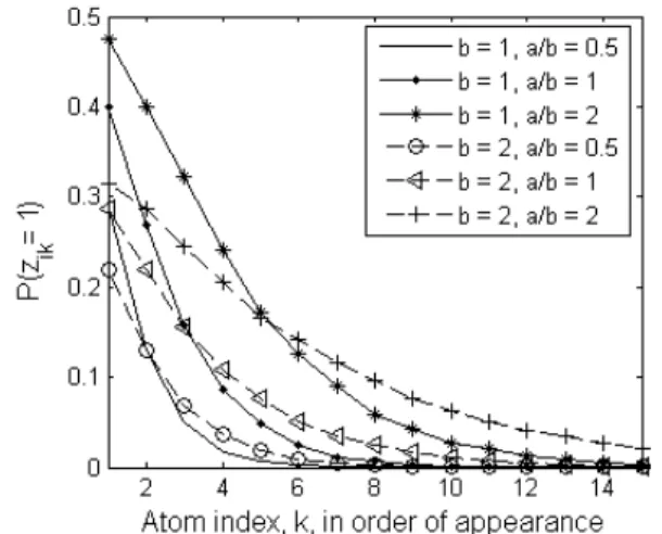
Figure 1.Estimation ofπfrom 5000 marginal beta process runs of 500 samples each, with variousa, binitializations.
We show in Figure 1 the expectation of π calculated empirically by drawing from the marginalized beta process. As can be seen, thea, bparameters offer flex-ibility in both the magnitude and shape ofπand can be tuned.
2.2. Finite Approximation to the Beta Process As hinted in (5), a finite approximation to the beta process can be made by simply setting K to a large, but finite number. This approximation can be viewed as serving a function similar to the finite Dirichlet dis-tribution in its approximation of the infinite Dirichlet process for mixture modeling. The finite representa-tion is written as
H(ω) = K X
k=1
πkδωk(ω)
πk ∼ Beta(a/K, b(K−1)/K) ωk
iid
∼ H0 (8)
with the K-dimensional vector, zi, drawn from a fi-nite Bernoulli process parameterized by H. The full conjugacy of this representation means posterior com-putation is analytical, which will allow for variational inference to be performed on the BP-FA model. We briefly mention that a stick-breaking construction of the beta process has recently been derived (Paisley & Carin, 2009), allowing for exact Bayesian inference. A construction for the Indian buffet process has also been presented (Teh et al., 2007), though this method does not extend to the more general beta process. We will use the finite approximation presented here in the following sections.
3. Beta Process Factor Analysis
Factor analysis can be viewed as the process of mod-eling a data matrix,X ∈RD×N, as the multiplication of two matrices, Φ∈RD×K andZ ∈
RK×N, plus an
error matrix, E.
X = ΦZ+E (9)
Often, prior knowledge about the structure of the data is used, for example, the desired sparseness properties of the Φ or Z matrices (West, 2003; Rai & Daum´e, 2008; Knowles & Ghahramani, 2007). The beta pro-cess is another such prior that achieves this sparseness, allowing forK to tend to infinity while only focusing on a small subset of the columns of Φ via the sparse matrixZ.
Inbeta process factor analysis (BP-FA), we model the matrices Φ andZasN draws from a Bernoulli process parameterized by a beta process, H. First, we recall that draws from the BeP-BP approximation can be generated as
zik ∼ Bernoulli(πk)
πk ∼ Beta(a/K, b(K−1)/K) φk
iid
∼ H0 (10)
for observation i = 1, . . . , N and latent feature (or factor) k = 1, . . . , K. In the general definition, H0
was unspecified, as was the use of the latent member-ship vector,zi. For BP-FA, we letH0 be multivariate
normal and the latent factors be indicators of linear combinations of these locations, which can be written in matrix notation as Φzi, where Φ = [φ1, . . . , φK]. Adding the noise vector,i, we obtain observationxi. The beta process can thus be seen as a prior on the parameters,{π,Φ}, with iid Bernoulli process samples composing the expectation matrix,E[X] = ΦZfor the factor analysis problem.
As an unweighted linear combination might be too restrictive, we include a weight vector, wi, which re-sults in the following generative process for observation i= 1, . . . , N,
xi = Φ(zi◦wi) +i wi ∼ N(0, σ2wI) zik ∼ Bernoulli(πk)
πk ∼ Beta(a/K, b(K−1)/K) φk ∼ N(0,Σ)
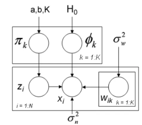
i ∼ N(0, σ2nI) (11) for k= 1, . . . , K and all values drawn independently. The symbol ◦ represents the Hadamard, or element-wise multiplication of two vectors. We show a graphi-cal representation of the BP-FA model in Figure 2.
Figure 2.A graphical representation of the BP-FA model.
Written in matrix notation, the weighted BP-FA model of (11) is thus a prior on
X = Φ(Z◦W) +E (12) Under this prior, the mean and covariance of a given vector,x, can be calculated,
E[x] = 0 E[xxT] =
aK a+b(K−1)σ
2
wΣ +σ
2
nI (13) LettingK → ∞, we see that E[xxT]→ abσ
2
wΣ +σn2I. Therefore, the BP-FA model remains well-defined in the infinite limit. To emphasize, compare this value with z removed, whereE[xxT] = Kσ2wΣ +σ
2
nI. The coefficient ab is significant in that it represents the ex-pected number of factors present in an observation as K → ∞. That is, if we define mi ≡ P∞k=1zik,
where zi ∼BeP(H) andH ∼BP(a, b, H0), then by
marginalizingH we find thatE[mi] = ab.
Another important aspect of the BP-FA model is that theπvector enforces sparseness on thesamesubset of factors. In comparison, consider the model where zi is removed and sparseness is enforced by sampling the elements ofwi iid from a sparseness inducing normal-gamma prior. This is equivalent to learning multi-ple relevance vector machines (Tipping, 2001) with a jointly learned and shared Φ matrix. A theoretical is-sue with this model is that the prior does not induce sparseness on the same subset of latent factors. As K → ∞, all factors will be used sparsely with equal probability and, therefore, no factors will be shared. This is conceptually similar to the problem of drawing multiple times from a Dirichlet process prior, where in-dividual draws are sparse, but no two draws are sparse on the same subset of atoms. We note that the hierar-chical Dirichlet process has been introduced to resolve this particular issue (Teh et al., 2006).
4. Variational Bayesian Inference
In this section, we derive a variational Bayesian algo-rithm (Beal, 2003) to perform fast inference for the weighted BP-FA model of (11). This is aided by the conjugacy of the beta to the Bernoulli process, where the posterior for the single parameter beta process is
H|X1, . . . , XN ∼BP αH0+
N X
i=1
Xi !
(14)
with Xi ∼ BeP(H) being the ith sample from a Bernoulli process parameterized by H. The two-parameter extension has a similar posterior update, though not as compact a written form.
In the following, we definex−ki ≡xi−Φ−k(z−ki ◦w −k i ), where Φ−k,z−k andw−k are the matrix/vectors with the kth column/element removed; this is simply the portion of xi remaining considering all but the kth factor. Also, for clarity, we have suppressed certain equation numbers and conditional variables.
4.1. The VB-E Step Update for Z:
p(zik|xi,Φ, wi, zi−k)∝p(xi|zik,Φ, wi, zi−k)p(zik|π) The probability thatzik= 1 is proportional to exp[hln(πk)i]×
exp
− 1 2σ2
n hw2
ikihφTkφki −2hwikihφkiThx−ki i
where h·i indicates the expectation. The probability that zik= 0 is proportional to exp[hln(1−πk)i]. The expectations can be calculated as
hln(πk)i = ψ a
K +hnki
−ψ
a+b(K−1)
K +N
hln(1−πk)i = ψ
b(K−1)
K +N− hnki
−ψ
a+b(K−1)
K +N
whereψ(·) represents the digamma function and hw2
iki = hwiki2+ ∆ 0(k)
i (15)
hφT
kφki = hφkiThφki+ trace(Σ0k) (16) where hnki is defined in the update for π, Σ0k in the update for Φ, and ∆0i(k)is thekth diagonal element of ∆0i defined in the update forW.
4.2. The VB-M Step Update for π:
p(πk|Z)∝p(Z|πk)p(πk|a, b, K)
The posterior ofπk can be shown to be πk ∼Beta
a
K +hnki,
b(K−1)
K +N− hnki
where hnki = PN
i=1hziki can be calculated from the VB-E step. The priors a, b can be tuned according to the discussion in Section 2.1. We recall that PN
i=1
a
b+i−1 is the expected total number of factors,
whilea/bis the expected number of factors used by a single observation in the limiting case.
Update for Φ:
p(φk|X,Φ−k, Z, W)∝p(X|φk,Φ−k, Z, W)p(φk|Σ) The posterior of φk can be shown to be normal with mean,µ0k, and covariance, Σ0k, equal to
Σ0k = 1 σ2 n N X i=1
hzikihw2ikiI+ Σ−1 !−1
(17)
µ0k = Σ0k 1 σ2
n N X
i=1
hzikihwikihx−ki i !
(18)
with hw2
iki given in (15). The prior Σ can be set to the empirical covariance of the data,X.
Update for W:
p(wi|xi,Φ, zi)∝p(xi|wi,Φ, zi)p(wi|σ2w)
The posterior of wi can be shown to be multivariate normal with mean,υ0i, and covariance, ∆0i, equal to
∆0i = 1
σ2
n
hΦ˜TiΦi˜ i+ 1 σ2
w I
−1
(19) υ0i = ∆0i
1 σ2
n hΦi˜ iTx
i
(20) where we define ˜Φi ≡ Φ◦Z˜i and ˜Zi ≡ [zi, . . . , zi]T, with the K-dimensional vector,zi, repeatedD times. Given thathΦi˜ i=hΦi ◦ hZ˜ii, we can then calculate
hΦ˜TiΦ˜ii= hΦiThΦi+A
◦ hziihziiT +Bi
(21) whereA andBi are calculated as follows
A ≡ diag [trace(Σ01), . . . ,trace(Σ0K)]
Bi ≡ diag [hzi1i(1− hzi1i), . . . ,hziKi(1− hziKi)] A prior, discussed below, can be placed on σ2
w, removing the need to set this value.
Update for σ2
n: p(σ2
n|X,Φ, Z, W)∝p(X|Φ, Z, W, σ2n)p(σn2) We can also infer the noise parameter,σ2
n, by using an inverse-gamma, InvGa(c, d), prior. The posterior can be shown to be inverse-gamma with
c0 = c+N D
2 (22)
d0 = d+1 2
N X
i=1
kxi− hΦi(hzii ◦ hwii)k2+ξi
where ξi≡
K X
k=1
hzikihw2ikihφ T
kφki − hziki2hwiki2hφkiThφki
+X k6=l
hzikihzili∆0i,klhφkiThφli In the previous equations, σ−2
n can then be replaced byhσ−2
n i=c0/d0. Update for σ2
w: p(σ2
w|W)∝p(W|σw2)p(σw2)
Given a conjugate,InvGa(e, f) prior, the posterior of σ2wis also inverse-gamma with
e0 = e+N K
2 (23)
f0 = f+1 2
N X
i=1
hwiiThwii+ trace(∆0i)
(24)
4.3. Accelerated VB Inference
As with the Dirichlet process, there is a tradeoff in variational inference for the BP-FA; the larger K is set, the more accurate the model should be, but the slower the model inference. We here briefly mention a simple remedy for this problem.
Following every iteration, the total factor membership expectations,{hnki}Kk=1, can be used to assess the
rel-evancy of a particular factor. When this number falls below a small threshold (e.g., 10−16), this factor index
can be skipped in following iterations with minimal impact on the convergence of the algorithm. In this way, the algorithm should converge more quickly as the number of iterations increases.
4.4. Prediction for New Observations
Given the outputs, {π,Φ}, the vectors z∗ and w∗ can be inferred for a new observation, x∗, using a MAP-EM inference algorithm that iterates between z∗ and w∗. The equations are similar to those detailed above, with inference forπand Φ removed.
5. Experiments
Factor analysis models are useful in many applications, for example, for dimensionality reduction in gene ex-pression analysis (West, 2003). In this section, we demonstrate the performance of the BP-FA model on synthetic data, and apply it to the MNIST digits and HGDP-CEPH cell line panel (Rosenberg et al., 2002) datasets.
5.1. A Synthetic Example
For our synthetic example, we generated H from the previously discussed approximation to the Beta pro-cess with a, b = 1, K = 100 and φk ∼ N(0, I) in a D = 25 dimensional space. We generated N = 250 samples from a Bernoulli process parameterized byH and synthesizedX withW = 1 andσ2
n= 0.0675. Be-low, we show results for the model having the highest likelihood selected from five runs, though the results in general were consistent.
In Figure 3, we display the ground truth (top) of Z, rearranged for display purposes. We note that only seven factors were actually used, while several obser-vations contain no factors at all, and thus are pure noise. We initialized our model to K = 100 factors, though as the results show (bottom), only a small sub-set were ultimately used. The inferred hσ2
ni= 0.0625 and the elementwise MSE of 0.0186 to the true ΦZ further indicates good performance. For this example, the BP-FA model was able to accurately uncover the underlying latent structure of the dataset.
Figure 3.Synthetic Data: Latent factor indicators,Z, for the true (top) and inferred (bottom) models.
5.2. MNIST Handwritten Digits Dataset We trained our BP-FA model on N = 2500 odd dig-its (500 each) from the MNIST digdig-its dataset. Us-ing PCA, we reduced the dimensionality to D= 350, which preserved over 99.5% of the total variance within the data. We truncated the BP-FA model toK= 100 factors initialized using the K-means algorithm and ran five times, selecting the run with the highest like-lihood, though again the results were consistent. In Figure 4 below, we show the factor sharing across the digits (left) by calculating the expected number of factors shared between two observations and normal-izing by the largest value (0.58); larger boxes indicate more sharing. At right, we show for each of the odd digits the most commonly used factor, followed by the second most used factorgiventhe factor to the left. Of particular interest are the digits 3 and 5, where they heavily share the same factor, followed by a factor that differentiates the two numbers.
In Figure 5 (top), we plot the sorted values of hπi inferred by the algorithm. As can be seen, the algo-rithm inferred a sparse set of factors, fewer than the 100 initially provided. Also in Figure 5 (bottom), we show an example of a reconstruction of the number 3 that uses four factors. As can be seen, no single factor can individually approximate the truth as well as their weighted linear combination. We note that the BP-FA model was fast, requiring 35 iterations on average to converge and requiring approximately 30 minutes for each run on a 2.66 GHz processor.
Figure 4.Left: Expected factor sharing between digits. Right: (left) Most frequently used factors for each digit (right) Most used second factor per digit given left factor.
Figure 5.(top) Inferred π indicating sparse factor usage. (bottom) An example reconstruction.
5.3. HGDP-CEPH Cell Line Panel
The HGDP-CEPH Human Genome Diversity Cell Line Panel (Rosenberg et al., 2002) is a dataset com-prising genotypes atD= 377 autosomal microsatellite loci sampled fromN = 1056 individuals in 52 popula-tions across the major geographic regions of the world. It is useful for inferring human evolutionary history and migration.
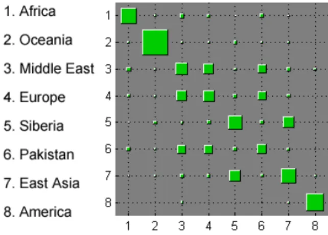
We ran our model on this dataset initializingK= 100 factors, though again, only a subset were significantly used. Figure 6 contains the sharing map, as previously calculated for the MNIST dataset, normalized on 0.55. We note the slight differentiation between the Middle East and European regions, a previous issue for this dataset (Rosenberg et al., 2002).
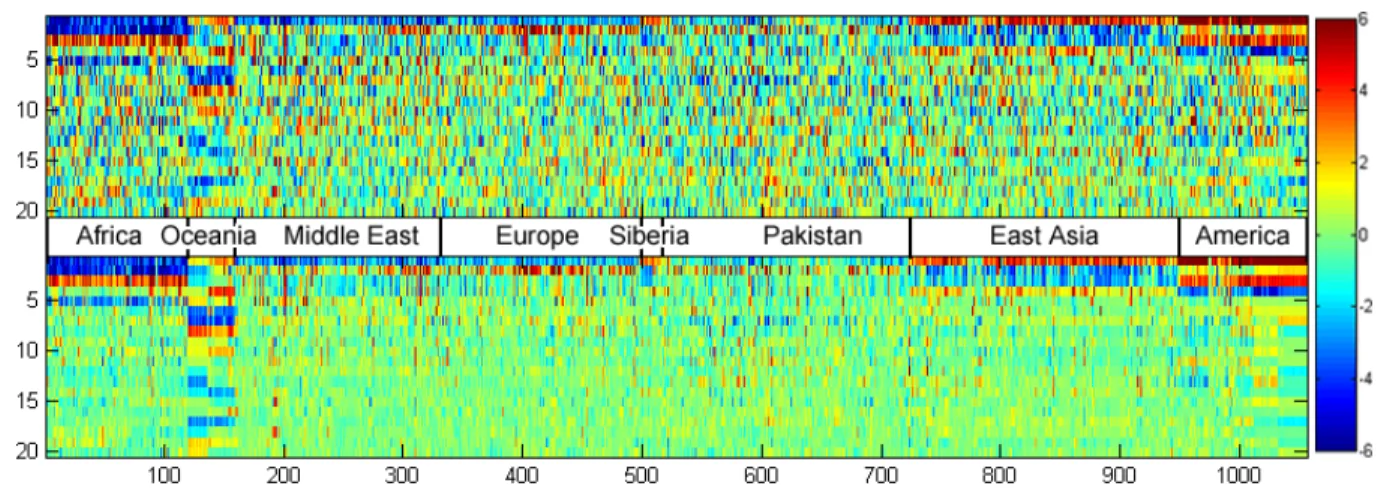
We also highlight the use of BP-FA in denoising. Fig-ure 8 shows the original HGDP-CEPH data, as well as the Φ(Z ◦W) reconstruction projected onto the first 20 principal components of the raw data. The figure shows how the BP-FA model was able to substantially reduce the noise level within the data, while still re-taining the essential structure.
Figure 6. Factor sharing across geographic regions.
Figure 7.Variance of HGDP-CEPH data along the first 150 principal components of the raw features for original and reconstructed data.
This is also evident in Figure 7, where we plot the variance along these same principal components for the first 150 dimensions. For an apparently noisy dataset such as this, BP-FA can potentially be use-ful as a preprocessing step in conjunction with other algorithms, in this case, for example, the Structure
(Rosenberg et al., 2002) or recently proposedmStruct
(Shringarpure & Xing, 2008) algorithms.
6. Conclusion and Future Work
We have proposed a beta process factor analysis (BP-FA) model for performing nonparametric factor anal-ysis with a potentially infinite number of factors. As with the Dirichlet process prior used for mixture mod-eling, the beta process is a fully Bayesian prior that as-sures the sharing of a sparse subset of factors among all observations. Taking advantage of conjugacy within the model, a variational Bayes algorithm was devel-oped for fast model inference requiring an approxima-tion comparable to the finite Dirichlet distribuapproxima-tion’s approximation to the infinite Dirichlet process. Re-sults were shown on synthetic data, as well as the MNIST handwritten digits and HGDP-CEPH cell line panel datasets.
While several nonparametric factor analysis models have been proposed for applications such as indepen-dent components analysis (Knowles & Ghahramani, 2007) and gene expression analysis (Rai & Daum´e, 2008; Meeds et al., 2007), these models rely on the Indian buffet process and therefore do not have fast variational solutions - an intended contribution of this paper. Furthermore, while the formal link has been made between the IBF and the beta process (Thibaux & Jordan, 2007), we believe our further development and application to factor analysis to be novel. In future work, the authors plan to develop a stick-breaking pro-cess for drawing directly from the beta propro-cess similar to (Sethuraman, 1994) for drawing from the Dirichlet process, which will remove the need for finite approx-imations.
Figure 8.HGDP-CEPH features projected onto the first 20 principal components of the raw features for the (top) original and (bottom) reconstructed data. The broad geographic breakdown is given between the images.
References
Aldous, D. (1985). Exchangeability and related topics.
´
Ecole d’ete de probabilit´es de Saint-Flour XIII-1983, 1–198.
Beal, M. (2003). Variational algorithms for approx-imate bayesian inference. Doctoral dissertation, Gatsby Computational Neuroscience Unit, Univer-sity College London.
Billingsley, P. (1995). Probability and measure, 3rd edition. Wiley Press, New York.
Ferguson, T. (1973). A bayesian analysis of some nonparametric problems. The Annals of Statistics, 1:209–230.
Griffiths, T. L., & Ghahramani, Z. (2005). Infinite latent feature models and the indian buffet pro-cess. Advances in Neural Information Processing Systems.
Hjort, N. L. (1990). Nonparametric bayes estimators based on beta processes in models for life history data. Annals of Statistics,18:3, 1259–1294.
Knowles, D., & Ghahramani, Z. (2007). Infinite sparse factor analysis and infinite independent components analysis. 7th International Conference on Indepen-dent Component Analysis and Signal Separation. Meeds, E., Ghahramani, Z., Neal, R., & Roweis, S.
(2007). Modeling dyadic data with binary latent factors. Advances in Neural Information Processing Systems.
Paisley, J., & Carin, L. (2009). A stick-breaking con-struction of the beta process (Technical Report). Duke University, ee.duke.edu/∼jwp4/StickBP.pdf.
Rai, P., & Daum´e, H. (2008). The infinite hierarchical factor regression model. Advances in Neural Infor-mation Processing Systems.
Rosenberg, N. A., Pritchard, J. K., Weber, J. L., Cann, H. M., Kidd, K. K., Zhivotovsky, L. A., & Feldman, M. W. (2002). Genetic structure of hu-man populations. Science,298, 2381–2385.
Sethuraman, J. (1994). A constructive definition of dirichlet priors. Statistica Sinica, 4:639–650. Shringarpure, S., & Xing, E. P. (2008). mstruct: A
new admixture model for inference of population structure in light of both genetic admixing and al-lele mutation. Proceedings of the 25th International Conference on Machine Learning.
Teh, Y. W., G¨or¨ur, D., & Ghahramani, Z. (2007). Stick-breaking construction for the indian buffet process.Proceedings of the International Conference on Artificial Intelligence and Statistics.
Teh, Y. W., Jordan, M. I., Beal, M. J., & Blei, D. M. (2006). Hierarchical dirichlet processes. Journal of the American Statistical Association, 101:1566– 1581.
Thibaux, R., & Jordan, M. I. (2007). Hierarchical beta processes and the indian buffet process. In-ternational Conference on Artificial Intelligence and Statistics.
Tipping, M. E. (2001). Sparse bayesian learning and the relevance vector machine. The Journal of Ma-chine Learning Research, 1:211–244.
West, M. (2003). Bayesian factor regression models in the “large p, small n” paradigm.Bayesian Statistics,