Multiplication on a Twisted Edwards Curve
with an Efficiently Computable Endomorphism
Zhe Liu1, Husen Wang2, Johann Großsch¨adl1, Zhi Hu3, and Ingrid Verbauwhede1
1
LACS, University of Luxembourg, Luxembourg
{zhe.liu,johann.groszschaedl}@uni.lu
2
ESAT/COSIC and iMinds, KU Leuven, Belgium
{husen.wang,ingrid.verbauwhede}@esat.kuleuven.be
3
Central South University, P.R. China
Abstract. The verification of an ECDSA signature requires a double-base scalar multiplication, an operation of the formk·G+l·Qwhere Gis a generator of a large elliptic curve group of prime ordern,Qis an arbitrary element of said group, andk,l are two integers in the range of [1, n−1]. We introduce in this paper an area-optimized VLSI design of a Prime-Field Arithmetic Unit (PFAU) that can serve as a loosely-coupled or tightly-loosely-coupled hardware accelerator in a system-on-chip to speed up the execution of double-base scalar multiplication. Our design is optimized for twisted Edwards curves with an efficiently computable endomorphism that allows one to reduce the number of point doublings by some 50% compared to a conventional implementation. An example for such a special curve is−x2+y2= 1 +x2y2 over the 207-bit prime fieldFp withp= 2207−5131. The PFAU prototype we describe in this paper features a (16×16)-bit multiplier and has an overall silicon area of 5821 gates when synthesized with a 0.13µstandard-cell library. It can be clocked with a frequency of up to 50 MHz and is capable to perform a constant-time multiplication in the mentioned 207-bit prime field in only 198 clock cycles. A complete double-base scalar multiplication has an execution time of some 365k cycles and requires the pre-computation of 15 points. Our design supports many trade-offs between performance and RAM requirements, which is a highly desirable property for future Internet-of-Things (IoT) applications.
Keywords: Signature verification, Twisted Edwards curve, Endomor-phism, Multiple-precision arithmetic, Pseudo-Mersenne prime
1
Introduction
client too. More specifically, TLS can provide server authentication by means of a certificate that binds an identity (e.g. the server’s domain name) to a pub-lic key. The certificate contains besides the ID and pubpub-lic key also a collection of attributes, all of which is signed by a trusted third party called Certification Authority (CA). In the initial (i.e. handshake) phase of the TLS protocol, the client normally requests the server’s certificate, and if he manages to verify the signature of the CA successfully, he is assured that the public key contained in the certificate is authentic and indeed belongs to the server. The next step is then to establish a shared secret between client and server, which can be done through either RSA-based key transport or via Diffie-Hellman key exchange. In any case, without prior authentication, the key establishment process would be vulnerable to a classical Man-In-The-Middle (MITM) attack. The same holds for Datagram TLS (DTLS) [25], a variant of TLS optimized for connectionless datagram transport (i.e. UDP) that is widely considered as the future standard protocol for securing the Internet of Things (IoT) [16].
The signature algorithms supported by the most recent version (i.e. version 1.2) of TLS are RSA [26], DSA [22], as well as ECDSA [14] through a separate RFC [3]. In order to validate the server’s certificate (or its chain of certificates [6]), the client needs to verify one or more signatures. Using RSA as signature algorithm has the advantage that verification is relatively fast since it involves an exponentiation by the public exponent, which is usually small (e.g. 216+ 1) [26]. However, the downside of RSA signatures is their size and accompanying memory and bandwidth requirements, especially at higher security levels. This can be exemplified with [30], where RSA with a modulus length of 3248 bits is recommended to match the security of 128-bit AES, which means an RSA sig-nature has a length of 406 bytes. Sigsig-natures of such a size can pose a problem for resource-constrained IoT devices that often have only a few hundred bytes to a few kB of RAM. On the other hand, Elliptic Curve Cryptography (ECC) is well-known for its compact key and signature sizes, which is a highly desirable feature for resource-limited devices. For example, a 255-bit ECDSA signature (matching the security of 128-bit AES) has a size of merely 64 bytes when it is compressed [2], i.e. less than one sixth of the RSA signature size. However, an inherent problem with ECDSA signatures is that, despite their small size, the verification process is relatively computation-intensive.
on a twisted Edwards curve [1] that allows for a more efficient implementation of the point arithmetic than a basic Weierstraß curve. Using a window method to reduce the number of point additions in a double-base scalar multiplication (as described in [11, p. 109f]) falls into the second category. Another option to cut down the number of point operations is to exploit an efficiently computable endomorphism as explained in [10] for variable-base scalar multiplication. Also a combination of both approaches, namely using the twisted Edwards addition law on so-called GLS [9] and GLV-GLS [20] curves (both of which are defined overFp2 and possess endomorphisms) has been investigated in [19] and [7].
In this paper we introduce families of twisted Edwards curves with an effi-ciently computable endomorphism φand demonstrate how said endomorphism can be used to speed up the ECDSA verification process, whereby we focus on hardware implementation of double-base scalar multiplication. In particular, we will study implementation properties of the twisted Edwards curve
ET : −x2+y2= 1 +x2y2 (1)
(i.e. a = −1 and d = 1) over a prime field Fp, which is birationally equiva-lent over Fp to a so-called Gallant-Lambert-Vanstone (GLV) curve [10] of the form EW : y2=x3+ax (i.e. b = 0). Gallant et al. [10] were the first to de-scribe how an efficiently-computable endomorphismφcan be used to speed up a variable-base scalar multiplication on such curves. While the exploitation of an endomorphism is independent of the curve representation, we are, to the best of our knowledge, the first to provide an explicit formula for the computation of said endomorphism on a twisted Edwards curve with a= −1 and d= 1. If
P = (x, y) is a point on the curveET given by Equation (1), then we can com-pute φ(P) = (αx,1/y) where αis an element of order 4 in the underlying field
equation with e.g.a= 0 orb= 0, our curve has the advantage of a faster (and complete) addition law4. The major advantage of our curve over a conventional twisted Edwards curve is the existence of an efficiently computable endomor-phism. On the other hand, when compared with GLS or GLV-GLS curves, our curve ET has the advantage that it is defined over a conventional prime field
Fp and not over a quadratic extension fieldFp2. Extension fields are rarely sup-ported by commodity cryptographic libraries, which hampers the use of GLS or GLV-GLS curves in real-world applications. Furthermore, our curve has the virtue of being more resource-friendly since it requires only arithmetic modulo
p, whereasFp2 involves both base-field (i.e. modulop) arithmetic and extension-field arithmetic. Finally, it has to be taken into account that exploiting the 4-way endomorphism on GLV-GLS curves for double-base scalar multiplication is very expensive in terms of memory. Namely, when using the 4-way endomorphism, an
m-bit double-base scalar multiplication is performed through eight simultaneous quarter-length (i.e. roughly m/4-bit) scalar multiplications, which requires the pre-computation and storage of (at least) 128 points. Since a single point typi-cally occupies between 40 and 64 bytes in memory, this approach is not suitable for resource-constrained IoT devices.
The real-world benefit of our curve is the multitude of implementation op-tions and trade-offs between execution time and silicon area (when thinking about hardware implementation) or memory footprint (in the context of software implementation) it supports. Providing many options and trade-offs is particu-lary important for cryptographic schemes to be used in the Internet of Things (IoT) since IoT devices come in all shapes and sizes, and have, therefore, varying resource constraints. At one end of the spectrum are devices with extreme re-strictions (e.g. RFID tags, sensor nodes) where every single gate and very single byte counts. At the other end of the spectrum are devices equipped with powerful 32-bit processors and plenty of resources. Our curve offers many implementation options that allow a designer to fine-tune an implementation according to the requirements at hand. For example, when resources are constrained, one can perform a double-based scalar multiplication in the straightforward fashion by computing two simultaneousm-bit scalar multiplication, which is very economic in terms of memory. On the other hand, if more resources are available, our curve allows the designer to trade performance for memory or area (depending on whether the implementation is in software or hardware) by exploiting the efficiently-computable endomorphism. Finally, if resources are plenty, it is possi-ble to achieve further speed-ups by combining the endomorphism with a window method for simultaneous scalar multiplication.
4
2
Twisted Edwards Curves with Endomorphism
2.1 Twisted Edwards Curve
Twisted Edwards curves were introduced to cryptography in 2008 [1] and are nowadays well established and become increasingly adopted in practical appli-cations due to their efficient addition law. LetFp be a prime field withp >3. A twisted Edwards curve overFpcan be defined as
Ea,d:ax2+y2= 1 +dx2y2, (2) whereaanddsatisfyad(a−d)6= 0. As specified in [1], thej-invariant ofEa,d is
j(Ea,d) =
16(a2+ 14ad+d2)3
ad(a−d)4 .
There is a remarkable addition law on twisted Edwards curves, which can be complete when a is a square andd a non-square inFp [1]. Here, completeness means the addition produces the correct result for any two points (even if one of the points is the neutral elementO= (0,1)) onEa,d, without exception.
2.2 GLV Method
Gallant, Lambert, and Vanstone [10] described in 2001 a new method (the so-called GLV method) for speeding up point multiplication on certain classes of elliptic curves, namely curves with an efficiently computable endomorphism. Let
E be an elliptic curve over a finite fieldFp and letG∈E(Fp) have prime order
n. Assuming that an efficiently computable endomorphism φ on E exists so that φ(G) = [λ]G∈ hGi, the GLV method replaces the computation [k]Gby a multi-scalar multiplication of the form [k1]G+ [k2]φ(G), where the sub-scalars
|k1|,|k2| ≈r1/2. Since the number of doublings is halved, this method potentially allows for significant speedup of the point multiplication.
Gallant et al. described in [10] several families of curves featuring an ef-ficiently computable endomorphism derived from special Complex Multiplica-tion (CM). Let φ be a complex number and K be the extension field Q(φ). If such an elliptic curve admits a complex multiplication by φ, then by [5, Thm 10.14] we obtain an endomorphismφ(x, y) = (φ−2f(x)
g(x), yφ −3f(x)
g(x)
0
) and
φ(O) = O, where f, g are polynomial functions over Q with degf =NK/Q(φ) and degg=NK/Q(φ)−1 (hereNK/Q(·) is the norm function fromK toQ).
2.3 Efficient Endomorphism on Twisted Edwards Curve
equivalence map can be given as
ψ :Ea,d→Es,(xt, yt)→(xs, ys) = (
c1(1 +yt) 1−yt
+c2,
c1(1 +yt)
xt(1−yt)
), (3)
ψ−1:Es→Ea,d,(xs, ys)→(xt, yt) = (
xs−c2
ys
,xs−c3 xs+c4
), (4)
withc1= (a−d)/4,c2= (a+d)/6,c3= (5a−d)/12, andc4= (a−5d)/12. The original GLV method works on some elliptic curves in Weierstrass model with special complex multiplication, e.g. curves having CM discriminant D =
−3,−4,−7,−8, etc. If there exists an efficient endomorphism φ on the curve
Es, then we can obtain an corresponding endomorphismφton the birationally-equivalent twisted Edwards curveEa,d asψ−1φψ. Thus, the GLV method is also applicable on twisted Edwards curves with some efficient endomorphism.
Usually, the computation of endomorphisms in the short Weierstrass model is much simpler than in the twisted Edwards model. In the following, we take the most common cases of “GLV friendly” curves (namely curves withj-invariant 0 and 1728) as examples.
J-invariant 0 Case. This class of elliptic curves has CM discriminantD=−3 and can be represented by a Weierstrass equation of the form
Eb: y2=x3+b (5) over a prime fieldFpwithp≡1 mod 3, which meansFpcontains an elementβof order 3. In this case, the mapφ:Eb→Eb given by (x, y)7→(βx, y) andO 7→ O is an endomorphism defined overFp. IfG∈Eb(Fp) is a point of prime ordern, thenφ(G) =λ·G= (βx, y), whereλis an integer satisfyingλ2+λ+1≡0 modn. There are only six possible group orders for such curves for a given fieldFp.
We can find a twisted Edwards curve birationally equivalent to the GLV curve Eb with help of the equation for the j-invariant: j(Ea,d) = 0 requires
a2+ 14ad+d2= 0, and when we fixato−1 then d=−7±4√3. Thus, we can obtain an endomorphism on its birationally equivalent twisted Edwards curve
Ea,d as
φt(x, y) = (
x(c5y+c6)
y+ 1 ,
c7y+c8
y+c9
), (6)
where c5 = 5dβ3(−2dd+1)+β+2, c6 = dβ+23(dd+1)+5β−2, c7 = (55dβd+1)(+d+ββ−+51), c8 = 55+d+1d and
c9= dβ(5d+5+1)(d+5ββ−+11).
J-invariant 1728 Case. Elliptic curves with a j-invariant of 1728 have CM discriminantD=−4 and can be defined by a Weierstrass equation of the form
over a prime field Fp with p ≡1 mod 4, i.e. it is guaranteed that Fp contains an elementαof order 4. In this case, the map φ:Ea →Ea given by (x, y)7→ (−x, αy) andO 7→ O is an endomorphism defined overFp. WhenG∈Ea(Fp) is a point of prime order n, thenφ(G) =λ·G= (−x, αy), whereλ is an integer satisfyingλ2+ 1≡0 modn. There are only four possible group orders for such curves whenFp is fixed.
Similar as before,j(Ea,d) = 1728 requires (a+d)(a2−34ad+d2) = 0, and when setting a = −1, we get d= 1 or d = 17±12√2. In the latter case, we can obtain an endomorphism φt on the corresponding twisted Edwards model
Ea,d:−x2+y2= 1 +dx2y2 in the same way as in thej-invariant 0 case. More concretely, whend= 17±12√2, the endomorphismφtcan be computed as
φt(x, y) = (−
x((7d−1)y+ (7−d)) 3α(d+ 1)(y+ 1) ,
(2d−2)y+ 5 +d
(5d+ 1)y+ (2−2d)). (8) On the other hand, ifd= 1,φt has a particularly simple formula, namely
φt(x, y) = (αx,1/y). (9)
The computation ofφtrequires only one multiplication and one inversion inFp. Consequently, computingφtonE−1,1:−x2+y2= 1+x2y2is much simpler (and faster) than computing the endomorphism(s) on the twisted Edwards GLV-GLS curves given in [20, Section 5].
3
Curve Generation
3.1 CM Method
LetE/Fpbe our desired elliptic curve with CM discriminantD. The group order of E/Fp is #E(Fp) = p+ 1−t, where t is the Frobenius trace. We also have the CM equation as 4p = t2−Ds2, where s ∈ Z. Note that the j-invariant
of such curve is also determined, and there are only 2 or 4 or 6 possible group orders for desired curve. Thus, the goal of the curve generation is not to find curve parameters (since we have them already), but rather to find a prime fieldFp, and then a twisted Edwards curve defined overFp (given bya=−1 and some fixed
d) which contains a large cyclic subgroup and meets other security requirements. This contrasts with the “traditional” approach for curve generation where the field Fp is fixed and one has to find suitable curve parameters.
3.2 Example Curve
We choose elliptic curve with CM discriminant D =−4 as our example. If we fix a = −1 for efficiency reasons [1], then by the analysis in Section 2.3, the possible value ofdis 1 or 17±12√2. We finally choose d= 1 since in this case the endomorphism onE−1,1 has a very simple formula as analyzed before.
Our example curve is
where the primep= 2207−5131. Note thatp≡1 mod 4, thenE
−1,1is ordinary. The group order #E−1,1(Fp) = 8·n, wheren= 0xFFFFFFFFFFFFFFFFFFF FFFFFFE090B67A2AE9D8EC7DD7009F95 is a 204-bit prime. Thus our curve is at around 100-bit security level. The embedding degree of E−1,1/Fp with respect to nisn−1, which means that it is resistant to the FR-MOV attack.
There is an efficient endomorphismφtonE−1,1 as
φt(x, y) = (α·x,1/y),
where α = 0x5135DD9F4EBC5D1835EFB3D377F3A4A1FCB1E2DEC2911FF 2B59A satisfies α2+ 1 ≡ 0 modp. And we can check that φ
t(G) = [λ]G for
G∈E−1,1(Fp) with λ= 0xA1D776BEDB1ECFFCE5ABB8F12F8223CC0F494 D461EC0F724D06, hereλ2+ 1≡0 modn.
4
Double-Base Scalar Multiplication
As mentioned before, double-base scalar multiplication is the most time-consum-ing operation of ECDSA signature verification and, therefore, deserves efficient implementation and optimization. Formally,double-base scalar multiplication is an operation of the form k·G+l ·Q and computes the sum of two scalar products, where G is fixed and Q is an arbitrary point. In the following, we review several approaches for performing the double-base scalar multiplication and describe how to speed up this operation by exploiting an endomorphism. For convenience, we assume that both scalars kandl are exactlymbits long.
Two Single Scalar Multiplications. The most straightforward method to perform the double-base scalar multiplication is to do the two single scalar mul-tiplications separately and then add up the results. The first scalar multiplication
k·G takes a fixed and a-priori-known point as input, which can be efficiently performed through the fixed-base comb method as described in [11, Section 3.3.2]. This single scalar multiplication requires roughly m/w point doublings and m(2w·w2−w1) point additions when using 2
w−1 pre-computed points, where w is the window size. The second scalar multiplication,l·Q, is performed with an arbitrary base pointQnot known in advance. When using a binary method, this arbitrary-base scalar multiplication requires to execute m point doublings and
m/2 point additions in average. In total, the double-base scalar multiplication requiresroughly m+m/w point doublings andm/2 + m(2w·w2−w1) point additions.
Interleaving Method. A method to speed up the computation ofk·G+l·Qis to perform them in a simultaneous (or interleaved) fashion by using a technique known as Shamir’s Trick [11, p. 109]. This method first computes the sum of
Joint Sparse Form. Solinas [31] proposed a joint sparse form (JSF) represen-tation of a pair of integers, which has the minimal joint Hamming weight. This representation can thus be used to speed up double-base scalar multiplication
k·G+l·Qby pre-computingS=G+QandD=G−Q. When taking advantage of JSF representation for the scalarskandl, a double-base scalar multiplication performed in an interleaved fashion requiresroughlympoint doublings andm/2 point additions (resp. subtractions) [11, Section 3.3.3].
(Sliding) Window Method. Another approach to reduce the number of point additions in a double-base scalar multiplication is to use a window method. Given the fixed window width w, a double-scalar multiplication first generates a look-up table with pointsi·G+j·Qfor alli, j∈[0,2w−1], and then scanswcolumns of the scalarskandl. This method requires storage of 22w−1 points and then a double scalar multiplication can be performed with roughly (m/w−1)·wpoint doublings and m(2w·22w2−w1)−1 point additions. The window method can be further
improved by using a “sliding” window; in this case, only 22w−22(w−1) points are actually needed for the look-up table, and the number of point additions is reduced to w+(1m/3) [11].
Double-Base Scalar Multiplication with Endomorphism
A maximum ofmpoint doublings can be saved for a double-base scalar multipli-cation when using the above described approaches. In the following, we present a strategy to further reduce the number of point doublings by some 50% using an efficiently computable endomorphism.
The main idea is to compute a double-base scalar multiplication, i.e.,k·G+
l·Q, through four simultaneous scalar multiplicationsk1·G,k2·φ(G),l1·Qand
l2·φ(Q), wherek1,k2,l1 andl2 are roughlym/2 bits long. Algorithm 1 shows the computation of double-base scalar multiplication exploiting an efficiently-computable endomorphism. We first split the scalark into two partsk1 andk2 using [11, Algorithm 3.74], wherek1 andk2 have roughly half of the bitlength of
k; the second scalar lcan be decomposed intol1 andl2 in the same way. Then, we calculate the points φ(G) and φ(Q) fromGand Qby using the formula in Section 2, which requires one inversion and a few multiplications. After that, we generate the look-up table with 15 points (line 4). Finally, the four scalar multiplicationsk1·G+k2·φ(G) +l1·Q+l2·φ(Q) is performed simultaneously, i.e. in an interleaved fashion. A double-base scalar multiplication using Algorithm 1 requiresapproximately m/2 point doubling and 15m/32 + 11 point additions including the overhead for the generation of the look-up table.
5
Hardware Architecture and Implementation
Algorithm 1.Double-base scalar multiplication using an endomorphism
Input: Twom-bit scalarskandl, the fixed base pointGand an arbitrary pointQon the curveE(Fp) with endomorphism.
Output: Double-base scalar multiplicationk·G+l·Q.
1: Use [11, Algorithm 3.74] to find (k1;k2) ofkand (l1;l2) ofl. 2: Computeφ(G),φ(Q) usingGandQ.
3: G= (k1>0)?G: −G; φ(G) = (k2>0)?φ(G) :−φ(G);Q = (l1>0)?Q:−Q; φ(Q) = (l2>0)?φ(Q) :−φ(Q);
4: Generate look-up tableT with 15 points such thatT[i−1] = [(i3)&1]·φ(Q) + [(i2)&1]·Q+ [(i1)&1]·φ(G) + (i&1)·Gfor 1≤i≤15.
5: Letk1 =|k1|,k2 =|k2|,l1 =|l1|,l2 =|l2|andh=max{k1, k2, l1, l2}. 6: R=∞.
7: forifromhby 1 down to 0do 8: R←2R;
9: s←8·l2i+ 4·l1i+ 2·k2i+k1i; 10: if s >0then
11: R←R+T[s−1]. 12: end if
13: end for 14: return R.
platform (i.e.ccan be at most 16 bits in our case since we use a 16-bit datapath). The basic idea of fast reduction using a pseudo-Mersenne prime is to apply the congruence relation 2k≡cmodprepetitively during the reduction process. Suppose z = zH2k +zL is a 2k-bit integer, such as obtained as result of a multiplication of twok-bit integers. We can reducezwith respect topas follows
z=zH2n+zL modp≡zHc+zLmodp (10) Now z is already only slightly longer than k bits since c is small. To complete the reductionzmodp, we perform the multiplication byc in the same way and then at most one subtraction ofpis needed to get a result that is at mostkbits long. Our implementation uses the pseudo-Mersenne primep= 2207−5131.
Notation. We use the following notation in this paper: – n: the operand size (i.e.n= 207).
– w: the word size of the underlying processor (i.e.w= 16).
– m: bitlength of the scalar, i.e. the bitlength of the order of the generatorG. – A,B: two operands;A[i:j] represents bits at positionitoj of operandA. – R: productA·B, which is twice long as operandAor B.
Note that all arithmetic operations (except the Montgomery inverse5) we discuss in the following can be easily implemented in a highly regular fashion so that their execution time is completely independent of the actual value of the operands. Such constant execution time helps to thwart certain implementation attacks like timing analysis. Even though signature verification does not involve any secret values (and can, therefore, not leak any secrets), it still makes sense to implement the underlying field arithmetic in a regular way so that it can also be used for signature generation.
5.1 Modular Multiplication and Squaring
The modular multiplication is performed in three basic steps as shown in Al-gorithm 2. First, a conventional multi-precision multiplication is performed in a word-wise fashion based on the product-scanning technique as described in e.g. [11]. Then, we multiply the most significant 209 bits of the product bycand add the result to least significant 207 bits, which yields a result of (at most) 226 bits length. Finally, we multiply the most significant 19 bits bycand add the product to least significant 207 bits; the result is now at most 208 bits and, therefore, fits into m words. In order to achieve constant execution time, we always execute both reduction steps, even when the result is already fully reduced after the first step.
Algorithm 2.Modular multiplication forp= 2207−c Input: Two integersA[207 : 0],B[207 : 0], and modulusp Output: R=A·Bmodp
1: R=A·B
2: R=R[415 : 207]·c+R[206 : 0]{The 1streduction}
3: R=R[225 : 207]·c+R[206 : 0]{The 2ndreduction}
A modular squaring can be done more efficiently thanks to the symmetry of partial products. Thus, it is possible to save the computation of (nearly) half of the partial products.
5.2 Modular Inversion
Modular inversion is the most time-consuming field arithmetic operation. Tradi-tionally, the Extended Euclidean Algorithm (EEA) [11], Fermat’s technique [11], and the Montgomery modular inversion algorithm [15, 28] are used to compute an inverse. Our inversion is mainly based on the Montgomery modular inverse, but has been optimized for the pseudo-Mersenne primep= 2n−c.
Algorithm 3.Optimized Montgomery Modular Inversion for 2n−c
Input: a∈[1,2n) and is odd,p >2 is anbits prime, precomputedT = 2(−2n)modp; Output: R∈[1,2n), whereR=a−1modp
1: //Phase I
2: u=−p,v=a,r= 0,s= 1,k= 0 3: while(1)do
4: x=u+v{Bothuandvare always odd number}
5: y=r+s
6: tlzx=DET(x){Trailing zero detection}
7: if x== 0then 8: break;
9: else if x <0then
10: u=x >> tlzx{Right-shift operation can be done in parallel withu+v}
11: r=y
12: s=s << tlzx{Left-shift operation can be done in parallel withr+s}
13: else
14: v=x >> tlzx 15: s=y
16: r=r << tlzx 17: end if
18: k=k+tlzx 19: end while 20: //phase II
21: s=s·2(2n−k)modp 22: s=s·T modp 23: returnR=s
As shown in Algorithm 3, our inversion consists of phases; phase I and phase II. In phase I, we firstly perform two additions, and then update the variables
{u, v, r, s, k} according to the sign flag ofx. The trailing zero detection (DET) and right-shift operation x >> tlzx can be done in parallel with the addition of u+v. Furthermore, the left-shift operation of s << tlzx and r << tlzx can be done in parallel with the addition of y=r+s. In phase II, we perform two ordinary multiplications to get the modular inverse. The inputais set to be odd, but even if initiallyais even, it can be easily changed to be odd via a modular subtractionp−a. The core idea behind our optimized inversion is to remove all trailing zeros of (u+v) in every iteration, which keeps uandv always odd so that (u+v) converges to zero quickly.
Compared to the Multibit Shifting method proposed by Sava¸s et al in [29], we remove all those iterations for shift operation (i.e. the iterations whenuorv
length of variables{u, v, r, s}to save cycles for addition, since the word lengths decrease linearly with the number of iterations.
5.3 Modular Addition and Subtraction
An addition modulo p = 2207−c can be performed in three steps. First, a conventional multi-precision addition R =A+B is performed in a word-wise fashion. Then, for reduction, we reduce the 209-bit result to 208 bits by using Equation (11). To ensure constant execution time, we perform the addition step and the reduction step for all possible inputs, even if no reduction is required.
R=R[209 : 207]·2207+R[206 : 0] modp=R[209 : 207]·c+R[206 : 0] (11) For modular subtraction, a conventional multi-precision subtractionR=A−B
is performed through word-wise subtract-with-borrow operations. As the 208-bit inputB can be bigger than 2p, the result of the subtraction may be smaller than−2pand, thus, up to two addition steps will be needed. As shown in Equa-tion (12), the first addiEqua-tion step will guarantee thatR >−p. IfRis still negative, another addition step as shown in Equation (13) will makeRa positive number in the range of [0,2208). To ensure constant execution time, we perform one sub-traction and two additions for all possible inputs, but whenR is positive after the subtraction, the words of the subtrahend with be masked out (i.e. set to 0) so that the value ofR does not change.
R=R+ 2p (12)
R=R+p (13)
5.4 Hardware Architecture
Controller ProgramROM
16*16
Mult Add/Sub
SRAM1
SRAM2
F207 Coprocessor
MULT R3, R1, R2
ADD R4, R6, R2
MSQ R5, R1
SUB R4, R5, R3 ...
Program
INV R4, R5
...
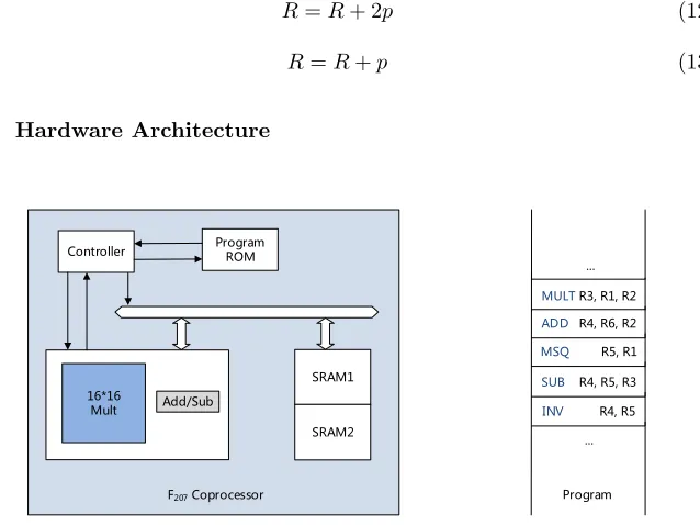
The hardware architecture, as shown in Fig 1, consists of a micro-controller, a program ROM, anFp-coprocessor, which we call Prime-Field Arithmetic Unit (i.e. PFAU), and two dual ports SRAMs. The program ROM is used to command sequences that execute high-level functions such as pre-computations, point ad-dition, point doubling, etc. This section focuses on the ALU.
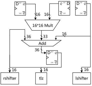
The architecture of the ALU and other important modules is shown in Fig-ure 2, where one (16×16)-bit multiplier, one 3-input adder, a trailing-zero de-tection module (tlz), a left-shifting module (lshifter), and a right-shifting module (rshifter) are depicted. We decided to implement a 16-bit datapath since previous research has shown that this allows one to achieve a good trade-off between performance and silicon area. The ALU supports the word-level instruc-tions needed for modular multiplication, modular squaring, modular inversion, modular addition and modular subtraction. The critical path goes from the in-put registers of the multiplier to the outin-put registers of the adder. The inin-put from mult to the adder is 33 bits long due to the fact that we need to double some partial products when performing a modular squaring.
The optimized modular inversion requires thetlz,lshifter,rshifter mod-ules. Using the implementation technique from [23], thetlzmodule can output the number of trailing zeros of a word (16 bits) in one clock cycle. To obtain the trailing zeros in a 208-bit operand, we can perform a zero detection word by word. If the number of trailing zeros exceeds one word, the detection process will take more than one cycle, but the probability is only 2−16 that we have a number with 16 trailing zeros (in fact, the probability is 2−15in our case sincex
is always even in Algorithm 3). Thelshifterandrshifterreceive the output of tlzperform the corresponding number of shifts on the 16-bit number input. As mentioned before, the shift operation in the modular inverse can be done in parallel with the addition.
Q Q
SET
CLR
D
Q QSET
CLR
D
Q Q
SET
CLR
D Add 16 16
16 36
36 16*16 Mult
Q Q
SET
CLR
D
33
rshifter tlz lshifter 16
16 16
All operations except modular inversion are designed for constant time, which also means worst-case calculation cycles. The execution time of modular inver-sion are evaluated based on the average number of Phase I iterations, with two additions per iteration and two modular multiplications in Phase II.
Microcode Based Architecture An alternative implementation option, which allows one to significantly reduce the ALU area, is to adopt a microcode based architecture, as mentioned in e.g. [13, 32, 24]. The ALU described in these works only supports word-size operations, such as 16 bits addition, subtraction, multi-plication, NOT, AND, OR and XOR. When following this approach, a microcode represents a sequence of commands sent to the ALU to perform certain oper-ations such as modular multiplication, modular addition, etc. Every operation corresponds to a sequence of commands, which will be stored in ROM. Thus, complex control logic for the field arithmetic, which is needed in the case of a hardwired in ALU, is mitigated to an upper software layer, which finally ends up in more ROM area for microcode storage. Considering that the size of ROM can be well optimized, this method can result in an overall area saving, but at the expense of a certain performance loss because due to inefficiency. Taking [13] as an example, the described implementation needs at least 32 clock cycles to per-form a 192-bit modular addition, without considering constant execution time. In summary, if one is willing to sacrifice some speed for a less complex ALU, then a microcode-based architecture may be an excellent option. According to our experiments, we could reduce the ALU area by roughly 30% when following a microcode approach.
6
Implementation Results
We implemented the arithmetic processor in Verilog and synthesized it with Design Compiler 2013.12 using the UMC 0.13µ 1P8M Low Leakage Standard cell Library with typical values (i.e. voltage of 1.2V and temperature of 25◦C). The area (in gate equivalents, GE) after placement and routing is calculated by dividing the overall area by the area of a single two-input NAND gate. The design has been synthesized for a clock frequency of 50M Hz, which is more than sufficient for common IoT devices such as FRID tags or sensor nodes.
6.1 Execution Time of Field Arithmetic
cycles. Thanks to the optimized Montgomery modular inversion proposed in Al-gorithm 3, our inversion requires 4452 clock cycles in average, which corresponds to only 23 multiplications.
Table 1. Execution time of field arithmetic operation using 16×16 multiplier over p= 2207−5131 (in clock cycles)
Operation Mul Sqr Inv Add Sub
This work 198 120 4452 30 43
6.2 Trade-offs between Performance and Memory
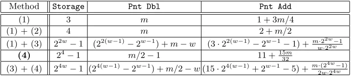
Table 2 reports the execution time and RAM requirements of double-base scalar multiplication for several different approaches as outlined in Section 4, as well as a combination of endomorphism and window method. Compared to the imple-mentation using (1), a double-base scalar multiplication using a combination of (1) and (2) requires the same number of point doubling while it saves approxi-mately 1/4 of the point additions. The number of point additions can be further reduced by using a combination of (1) and (3) with a look-up table of 22w−1 points. Taking the window width w = 2 as an example, one can save roughly 1/16 of the point additions compared to the implementation with a combination of (1) and (2). In relation to a combination of (1) and (3), the number of point doublings can be further reduced by some 50% using the technique of (4) with the same RAM occupation. A small number of point additions may potentially be saved by using a combination of (3) + (4). However, one has to consider that the look-up table will increase exponentially and a combination of (3) and (4) is only able to save point additions when n is big enough. For example, given
w = 2, a double-base scalar multiplication using a combination of (3) and (4) requires a look-up table of 255 points and even requires more point doublings and point additions. Taking both performance and RAM requirements into ac-count, the technique (4) (i.e. endomorphism) is the best choice to speed up the double-base scalar multiplication on resource-constraint platforms.
6.3 High-Speed Version vs Memory-Efficient Version
A double-base scalar multiplicationk·G+l·Qusing endomorphismφrequires to compute four simultaneous scalar multiplications of the formk1·G+k2·φ(G) +
Table 2.Comparison of execution time (including the generation of look-up table) and RAM requirements of double-base scalar multiplication using different approaches.
Method Storage Pnt Dbl Pnt Add
(1) 3 m 1 + 3m/4
(1) + (2) 4 m 2 +m/2
(1) + (3) 22w−1 (22(w−1)−2w−1) +m−w (3·22(w−1)−2w−1−1) +m·22w−1 w·22w
(4) 24−1 m/2−1 11 +1532m
(3) + (4) 24w−1 (24(w−1)−2w−1) +m/2−w(15·24(w−1)+ 2w−1−5) +m2·(2w4·2w4−w1)
(1): Interleaved; (2): JSF; (3): Window; (4): Endomorphism.
Speed-Optimized. The speed-optimized implementation requires a look-up table containing 15 points, of which 11 points (except G, Q, φ(G) and φ(Q)) will be generated by a sequence of point additions. In order to take the advan-tage of the efficient point addition formula on a twisted Edwards curve (i.e. the 7M mixed addition formulae based on [12]), we store these points in extended affine coordinate of the form (U, V, W), where U = (x+y)/2, V = (y−x)/2,
W =xy(in our cased= 1). A straightforward method to get the affine form of these points would require 11 inversions. For reducing the number of inversions, we perform the 11 inversions in a simultaneous way based on the observation that 1/x = y(1/xy) and 1/y = x(1/xy) [11, page 44]. With the help of three temporary variables, the 11 inversions can be computed by only one inversion and 83 multiplications. Given an affine point, the extended affine coordinates (U, V, W) can be obtained by performing one addition, one subtraction and one multiplication. In the main loop, a pre-computed point in extended affine coor-dinates will be used as operand in each iteration (i.e. line 7-13 of Algorithm 1). As a result, our speed-optimized double-base scalar multiplication requires an execution time of 365,082 clock cycles with a RAM footprint of 1612 bytes.
For comparison, a double-base scalar multiplication without exploiting the endomorphism (i.e. using just the straightforward simultaneous approach along with a JSF representation of the scalars) has a execution time of 454179 cycles, i.e. using the endomorphism yields a speed-up of roughly 20%.
on [12]). Thus, we compute the extended affine representation of an affine point on-the-fly, which requires one multiplication, one addition and one subtraction for each iteration. As a consequence, our memory-optimized double-base scalar multiplication requires an execution time of 415,392 clock cycles with a RAM consumption of only 1222 bytes, which corresponds to a saving of 33% for the look-up table (780 instead of 1170 bytes) and 24% in total (i.e. 1222 instead of 1612 bytes), by sacrificing only about 12.1% of performance.
6.4 Comparison with Other Implementations
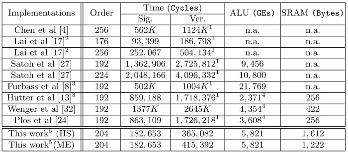
Table 3. Comparison of execution time, area and RAM consumption with related work over prime fields. Most of the work used a 16-bit datapath.
Time (Cycles) Implementations Order
Sig. Ver. ALU(GEs) SRAM(Bytes)
Chen et al [4] 256 562K 1124K1 n.a. n.a. Lai et al [17]2 176 93,399 186,7981 n.a. n.a. Lai et al [17]2 256 252,067 504,1341 n.a. n.a. Satoh et al [27] 192 1,362,906 2,725,8121 9,456 n.a. Satoh et al [27] 224 2,048,166 4,096,3321 10,800 n.a. Furbass et al [8]3 192 502K 1004K1 21,769 n.a. Hutter et al [13]3 192 859,188 1,718,3761 2,3714 256 Wenger et al [32] 192 1377K 2645K 4,3544 422 Plos et al [24] 192 863,109 1,726,2181 3,6084 256 This work5 (HS) 204 182,653 365,082 5,821 1,612 This work5(ME) 204 182,653 415,392 5,821 1,222
1: Estimated results from the execution time of signature implementation. 2
: Four 32 bits multipliers used. 3: 0.35µmtechnology library used. 4
: Microcode based architecture used, more ROM are required.
5: Execution time of fixed-base scalar multiplication (for signature generation) and double-base scalar multiplication (for verification).
hand, the memory-oriented implementation needs 415,392 clock cycles, while consuming only 1.2 kB of RAM. Since most of the previous implementations only reported the execution time of signature generation, we estimate the cycle count of verification (i.e. double-base scalar multiplication) by simply multiply-ing the generation time by two. As shown in the Table 3, our implementation is at least three times faster than all the previous works using the same word size. In terms of area, the implementations from [27] and [17] support both prime and binary field arithmetic and, thus, have a large area. On the other hand, the authors of [13, 32, 24] optimized their implementation with the help of a microcode-programmable structure (for field arithmetic) and, thus, their imple-mentations require extra instruction decoding modules and have higher ROM consumption in order to save area in the control logic. Our implementation does not include the area for SRAM since it varies for different process technologies and depends significantly on whether one has a RAM generator available or not. Besides, the needed SRAM may come from shared memory and just be temperately occupied during signature generation or verification.
7
Conclusions
In this work, we first introduced a special twisted Edwards curve with an ef-ficiently computable endomorphism and described how said endomorphism be exploited to speed up double-base scalar multiplication. As second contribution, we presented an area-optimized VLSI design of PFAU, an arithmetic unit fea-turing a (16×16)-bit multiplier that has an overall silicon area of 5821 gates when synthesized with a 0.13µstandard-cell library. Our PFAU can be clocked with a frequency of up to 50 MHz and is capable to perform a constant-time multiplication in a 207-bit prime field in only 198 clock cycles. We used PFAU as a vehicle to explore different trade-offs between memory and execution time, whereby we used the twisted Edwards curve−x2+y2= 1 +x2y2 over the 207-bit prime field Fp with p = 2207 −5131 as case study. In a speed-optimized setting, our implementation requires an execution time of 182,653 and 365,082 clock cycles for constant-time fixed-base scalar multiplication and double-base scalar multiplication, respectively. In addition, we showed that our curve sup-ports various trade-offs between execution time and memory requirements, which gives a designer plenty options to optimize double-base scalar multiplication for different requirements.
References
1. D. J. Bernstein, P. Birkner, M. Joye, T. Lange, and C. Peters. Twisted Edwards curves. In S. Vaudenay, editor,Progress in Cryptology — AFRICACRYPT 2008, volume 5023 ofLecture Notes in Computer Science, pages 389–405. Springer Ver-lag, 2008.
3. S. Blake-Wilson, N. Bolyard, V. Gupta, C. Hawk, and B. M¨oller. Elliptic Curve Cryptography (ECC) Cipher Suites for Transport Layer Security (TLS). Internet Engineering Task Force, Network Working Group, RFC 4492, May 2006.
4. G. Chen, G. Bai, and H. Chen. A high-performance elliptic curve cryptographic processor for general curves over GF(p) based on a systolic arithmetic unit.IEEE Transactions on Circuits and Systems II: Express Briefs, 54(5):412–416, 2007. 5. D. A. Cox. Primes of the Formx2+ny2. John Wiley & Sons, 1989.
6. T. Dierks and E. K. Rescorla. The Transport Layer Security (TLS) Protocol Version 1.2. Internet Engineering Task Force, Network Working Group, RFC 5246, Aug. 2008.
7. A. Faz-Hern´andez, P. Longa, and A. H. S´anchez. Efficient and secure algorithms for GLV-based scalar multiplication and their implementation on GLV-GLS curves. In J. Benaloh, editor,Topics in Cryptology — CT-RSA 2014, volume 8366 ofLecture Notes in Computer Science, pages 1–27. Springer Verlag, 2014.
8. F. Furbass and J. Wolkerstorfer. ECC processor with low die size for RFID ap-plications. In IEEE International Symposium on Circuits and Systems (ISCAS 2007), pages 1835–1838. IEEE, 2007.
9. S. D. Galbraith, X. Lin, and M. Scott. Endomorphisms for faster elliptic curve cryptography on a large class of curves. In A. Joux, editor,Advances in Cryptology — EUROCRYPT 2009, volume 5479 ofLecture Notes in Computer Science, pages 518–535. Springer Verlag, 2009.
10. R. P. Gallant, R. J. Lambert, and S. A. Vanstone. Faster point multiplication on elliptic curves with efficient endomorphism. In J. Kilian, editor, Advances in Cryptology — CRYPTO 2001, volume 2139 ofLecture Notes in Computer Science, pages 190–200. Springer Verlag, 2001.
11. D. R. Hankerson, A. J. Menezes, and S. A. Vanstone. Guide to Elliptic Curve Cryptography. Springer Verlag, 2004.
12. H. Hi¸sil, K. K.-H. Wong, G. Carter, and E. Dawson. Twisted Edwards curves revisited. In J. Pieprzyk, editor, Advances in Cryptology — ASIACRYPT 2008, volume 5350 ofLecture Notes in Computer Science, pages 326–343. Springer Ver-lag, 2008.
13. M. Hutter, M. Feldhofer, and T. Plos. An ECDSA processor for RFID authen-tication. In Radio Frequency Identification: Security and Privacy Issues, pages 189–202. Springer, 2010.
14. D. Johnson, A. J. Menezes, and S. A. Vanstone. The elliptic curve digital signature algorithm (ECDSA). International Journal of Information Security, 1(1):36–63, July 2001.
15. B. S. Kaliski. The Montgomery inverse and its applications. IEEE Transactions on Computers, 44(8):1064–1065, 1995.
16. S. L. Keoh, S. S. Kumar, and H. Tschofenig. Securing the Internet of things: A standardization perspective. IEEE Internet of Things Journal, 1(3):265–275, June 2014.
17. J.-Y. Lai and C.-T. Huang. A highly efficient cipher processor for dual-field elliptic curve cryptography.IEEE Transactions on Circuits and Systems II: Express Briefs, 56(5):394–398, 2009.
19. P. Longa and C. H. Gebotys. Efficient techniques for high-speed elliptic curve cryptography. In S. Mangard and F.-X. Standaert, editors,Cryptographic Hardware and Embedded Systems — CHES 2010, volume 6225 ofLecture Notes in Computer Science, pages 80–94. Springer Verlag, 2010.
20. P. Longa and F. Sica. Four-dimensional Gallant-Lambert-Vanstone scalar multipli-cation. In X. Wang and K. Sako, editors,Advances in Cryptology — ASIACRYPT 2012, volume 7658 ofLecture Notes in Computer Science, pages 719–739. Springer Verlag, 2012.
21. R. L´orencz and J. Hlav´aˇc. Subtraction-free almost Montgomery inverse algorithm.
Information Processing Letters, 94(1):11–14, 2005.
22. National Institute of Standards and Technology (NIST). Digital Signature Stan-dard (DSS). FIPS Publication 186-4, available for download athttp://nvlpubs. nist.gov/nistpubs/FIPS/NIST.FIPS.186-4.pdf, July 2013.
23. V. G. Oklobdzija. An algorithmic and novel design of a leading zero detector circuit: Comparison with logic synthesis. IEEE Transactions on Very Large Scale Integration (VLSI) Systems, 2(1):124–128, 1994.
24. T. Plos, M. Hutter, M. Feldhofer, M. Stiglic, and F. Cavaliere. Security-enabled near-field communication tag with flexible architecture supporting asymmetric cryptography. IEEE Transactions on Very Large Scale Integration (VLSI) Sys-tems, 21(11):1965–1974, 2013.
25. E. K. Rescorla and N. G. Modadugu. Datagram Transport Layer Security Version 1.2. Internet Engineering Task Force, Network Working Group, RFC 6347, Jan. 2012.
26. R. L. Rivest, A. Shamir, and L. M. Adleman. A method for obtaining digital signatures and public key cryptosystems.Communications of the ACM, 21(2):120– 126, Feb. 1978.
27. A. Satoh and K. Takano. A scalable dual-field elliptic curve cryptographic proces-sor. IEEE Transactions on Computers, 52(4):449–460, 2003.
28. E. Sava¸s. The Montgomery modular inverse—Revisited. IEEE Transactions on Computers, 49(7):763–766, 2000.
29. E. Sava¸s, M. Naseer, A.-A. Gutub, and C¸ . K. Ko¸c. Efficient unified Montgomery in-version with multibit shifting.IEE Proceedings–Computers and Digital Techniques, 152(4):489–498, 2005.
30. N. P. Smart, editor.ECRYPT II Yearly Report on Algorithms and Keysizes (2011-2012). European Network of Excellence in Cryptology (ECRYPT II), Sept. 2012. Deliverable D.SPA.20, available for download at http://www.ecrypt.eu.org/ documents/D.SPA.20.pdf.
31. J. A. Solinas. Low-weight binary representations for pairs of integers. Techni-cal Report CORR 2001-41, Centre for Applied Cryptographic Research (CACR), University of Waterloo, Waterloo, Canada, 2001.
32. E. Wenger, M. Feldhofer, and N. Felber. Low-resource hardware design of an elliptic curve processor for contactless devices. InInformation Security Applications, pages 92–106. Springer, 2011.
33. T. Yanık, E. Sava¸s, and C¸ . K. Ko¸c. Incomplete reduction in modular arithmetic.
IEE Proceedings – Computers and Digital Techniques, 149(2):46–52, Mar. 2002.
A
Constant-time Inversion over
p
= 2
207−
5131
z−1≡z2207−5133
modpby the following steps (where the annotations after the # denote the value of the exponent and the cost in each step).
z3←z2·z # 3,1S+ 1M
z6←z2 1
3 # 6,1S
z15←z2 1
6 ·z3 # 15,1S+ 1M
z31←z2 1
15·z # 2
5−1,1S+ 1M
t0←z2 4
31 # 2
9−24,4S
t1←t2 4
0 ·z15 # 29−1,1M
t2←t2 9
1 # 2
18−29,9S
t3←t2·t1 # 218−1,1M
t4←t2 5
3 ·z31 # 223−1,5S+ 1M
t5←t2 23
4 ·t4 # 246−1,23S+ 1M
t6←t2 46
5 ·t5 # 292−1,46S+ 1M
t7←t2 92
6 ·t6 # 2184−1,92S+ 1M
t8←(t2 14
7 ·z15·z6)2 4
# (2198−214+ 21)·24,18S+ 2M t9←(t8·t2)2
5