Form factor π0γ*γ in lightcone sum rules combined with renormalization-group summation vs experimental data.

Form factor

π

γ

γ

in lightcone sum rules combined with

renormalization-group summation vs experimental data.

C.Ayala1,∗_{,S.V. Mikhailov}2,∗∗_{,A.V. Pimikov}3,∗∗∗_{, andN.G. Stefanis}4,∗∗∗∗

1_{Department of Physics, Universidad Técnica Federico Santa María, Casilla 110-V, Valparaíso, Chile} 2_{Bogoliubov Laboratory of Theoretical Physics, JINR, 141980 Dubna, Russia}

3_{Institute of Modern Physics, Chinese Academy of Science, Lanzhou 730000, China}

4_{Ruhr-Universität Bochum, Fakultät für Physik and Astronomie, Institut für Theoretische Physik II,}

D-44780 Bochum, Germany

Abstract.We consider the lightcone sum-rule (LCSR) description of the pion-photon transition form factor in combination with the renormalization group of QCD. The emerging scheme represents a certain version of Fractional Ana-lytic Perturbation Theory and significantly extends the applicability domain of perturbation theory towards lower momentaQ2 _{1 GeV}2_{. We show that the}

predictions calculated herewith agree very well with the released preliminary data of the BESIII experiment, which have very small errors just in this region, while the agreement with other data at higherQ2_{is compatible with the LCSR}

predictions obtained recently by one of us using fixed-order perturbation theory.

1 Introduction.

In this work we consider the calculation of theπ0γ∗γtransition form factor (TFF) within the LCSR approach, see, e.g., [1, 2], going beyond fixed-order perturbation theory (FOPT). We use instead the approach worked out in [3], which combines the method of LCSRs, based on dispersion relations, with the renormalization-group (RG) summation, expressed in terms of the formal solution of the Efremov-Radyushkin-Brodsky-Lepage (ERBL) [4, 5] evolution equation. We argued [3] that this procedure gives rise to a particular version of fractional analytic perturbation theory (FAPT) [6, 7] within QCD—see [8, 9] for reviews.

From the calculational point of view, this FAPT-related approach helps avoid the appear-ance of large radiative corrections to the pion-photon TFF at low/moderate momenta. This

is because such terms become small by virtue of the FAPT summation in contrast to the currently known [2] FOPT results (up to the order ofO(α2_sβ0)). The emergent FAPT/LCSR

approach rearranges completely the perturbative QCD corrections turning them into a non-power series of FAPT couplings, see [3, 6, 7], which have no Landau singularities when

Q2 _Λ2

QCD. As a result, the domain of applicability of this perturbative expansion is

sig-nificantly extended towards lower momentum transfers. From the phenomenological point of view, the FAPT/LCSR approach extends the validity range of the TFF predictions below

∗_{e-mail: [email protected]} ∗∗_{e-mail: [email protected]} ∗∗∗_{e-mail: [email protected]}

Q2_{≤1 GeV}2_{, where the preliminary BESIII data on the pion TFF bear very small error bars}

[10]. This data regime cannot be reliably assessed using LCSRs within FOPT, showing a tendency to underestimate them below 1 GeV2_[11].

Consider now the pion-photon transition form factor for two highly virtual photons de-scribing the reactionγ∗(−Q2_)γ∗_(−q2_)→π0_{by assuming thatQ}2_,q2 _m2

ρ. Applying

factor-ization, the pion-photon transition form factorFγ∗_γ∗_π0

can be written in terms of convolutions of perturbatively calculable hard-scattering parton amplitudes T(n) _{of γ}∗_γ∗ _{→ q(Gµν)¯qand}

pion distribution amplitudes (DAs)ϕ(πn)of nonperturbative nature to get Fγ∗_γ∗_π0

(Q2_,q2_{, µ}2_{) ∼T}(2)_(Q2_,q2_{, µ}2_;x)⊗

xϕ

(2)

π (x, µ2)+ (1)

T(4)_(Q2_,q2_{, µ}2_;x)⊗

xϕ

(4)

π (x, µ2)+inverse-power corr. like twist-6, (2)

where⊗_x ≡∫₀1dxand the superscript (n) denotes the twist label. We have adopted the default scale setting by identifying the factorization (label F) and renormalization (label R) scale µF=µR=µ. It is possible to sum the infinite series of the logarithmic corrections associated

with the couplingas =αs(µ2)/4πand theϕπ(x;µ2) renormalization by absorbing them into

the new argument of the running coupling ¯as(q2_y¯+Q2_{y) ≡ a¯s(y) and the ERBL exponent}

for the DAs, respectively. For further details we refer to the discussion given in Sec. II of [3] and references cited therein. The ERBL exponent accumulates all ERBL evolution kernels

ak+1

s Vk, while only the coefficient functionsaksT(k)of the parton subprocesses remain in the perturbative expansion of the leading-twist amplitudeT(2)_.

It is useful to consider the twist-two pion DA, as well as the corresponding contribution to the TFF in (1), as an expansion in the conformal basis of the Gegenbauer harmonics{ψn(x)=

6xxC¯ n3/2(x−x¯)},

ϕ(2)π (x, µ2) = ψ0(x)+ ∞ ∑

n=2,4,...

an(µ2)ψn(x), (3a)

F(tw=2)_(Q2_,q2_{) = F}(tw=2)

0 (Q2,q2)+ ∞ ∑

n=2,4,...

an(µ2)F(tw=2)

n (Q2,q2). (3b)

At the one-loop level, the next-to-leading-order (NLO) coefficient function isT(1) and the

RHS of Eq. (1) for the twist-two contribution reduces in the{ψn}basis to

F(tw=2)

n (Q2,q2)

1-loop −→ F(tw=2)

(1l)n =NTT0(y)⊗_y

{[

1l+a¯s(y)T(1)(y,x)] (a¯s(y) as(µ2₎

)νn}

⊗_xψn(x).(4)

In the above equation,T0(y) is the Born term of the perturbative expansion forT(2), while the

other used notations mean

T0(y)≡T0(Q2,q2;y)=_q2y¯+1_Q2y; 1l=δ(x−y); NT = √2fπ/3; (5)

V(as;y,z)→asV0(y,z); V0(y,z)⊗ψn(z)=−1

2γ0(n)ψn(y); β(α)→ −a2sβ0, (6)

whereasγ0(n) denotes the one-loop anomalous dimension of the corresponding composite

operator of leading twist withνn = 1 2

γ0(n)

β0 . It is important to appreciate that Eq. (4) has

no sense for smallq2_{even ifQ}2_{is large. Indeed, the scale argumentq}2_y¯+Q2_yapproaches

for y _→ 0 the small q2 _{regime, so that the perturbative expansion becomes unprotected.}

Q2 _{≤1 GeV}2_{, where the preliminary BESIII data on the pion TFF bear very small error bars}

[10]. This data regime cannot be reliably assessed using LCSRs within FOPT, showing a tendency to underestimate them below 1 GeV2_[11].

Consider now the pion-photon transition form factor for two highly virtual photons de-scribing the reactionγ∗(−Q2_)γ∗_(−q2_)→π0_{by assuming thatQ}2_,q2_m2

ρ. Applying

factor-ization, the pion-photon transition form factorFγ∗_γ∗_π0

can be written in terms of convolutions of perturbatively calculable hard-scattering parton amplitudes T(n) _ofγ∗_γ∗ _{→ q(Gµν)¯qand}

pion distribution amplitudes (DAs)ϕ(πn)of nonperturbative nature to get Fγ∗_γ∗_π0

(Q2_,q2_{, µ}2_{) ∼T}(2)_(Q2_,q2_{, µ}2_;x)⊗

x ϕ

(2)

π (x, µ2)+ (1)

T(4)_(Q2_,q2_{, µ}2_;x)⊗

x ϕ

(4)

π (x, µ2)+inverse-power corr. like twist-6, (2)

where⊗_x ≡∫₀1dxand the superscript (n) denotes the twist label. We have adopted the default scale setting by identifying the factorization (label F) and renormalization (label R) scale µF=µR=µ. It is possible to sum the infinite series of the logarithmic corrections associated

with the couplingas =αs(µ2)/4πand theϕπ(x;µ2) renormalization by absorbing them into

the new argument of the running coupling ¯as(q2_y¯+Q2_{y) ≡ a¯s(y) and the ERBL exponent}

for the DAs, respectively. For further details we refer to the discussion given in Sec. II of [3] and references cited therein. The ERBL exponent accumulates all ERBL evolution kernels

ak+1

s Vk, while only the coefficient functionsaksT(k)of the parton subprocesses remain in the perturbative expansion of the leading-twist amplitudeT(2)_.

It is useful to consider the twist-two pion DA, as well as the corresponding contribution to the TFF in (1), as an expansion in the conformal basis of the Gegenbauer harmonics{ψn(x)=

6xxC¯ 3/2n (x−x¯)},

ϕ(2)π (x, µ2) = ψ0(x)+ ∞ ∑

n=2,4,...

an(µ2)ψn(x), (3a)

F(tw=2)_(Q2_,q2_{) = F}(tw=2)

0 (Q2,q2)+ ∞ ∑

n=2,4,...

an(µ2)F(tw=2)

n (Q2,q2). (3b)

At the one-loop level, the next-to-leading-order (NLO) coefficient function isT(1) and the

RHS of Eq. (1) for the twist-two contribution reduces in the{ψn}basis to

F(tw=2)

n (Q2,q2)

1-loop −→ F(tw=2)

(1l)n =NTT0(y)⊗_y

{[

1l+a¯s(y)T(1)(y,x)] ( a¯s(y) as(µ2₎

)νn}

⊗_xψn(x). (4)

In the above equation,T0(y) is the Born term of the perturbative expansion forT(2), while the

other used notations mean

T0(y)≡T0(Q2,q2;y)=_q2y¯+1_Q2y; 1l=δ(x−y); NT= √2fπ/3; (5)

V(as;y,z)→asV0(y,z); V0(y,z)⊗ψn(z)=−1

2γ0(n)ψn(y); β(α)→ −a2sβ0, (6)

whereasγ0(n) denotes the one-loop anomalous dimension of the corresponding composite

operator of leading twist with νn = 1 2

γ0(n)

β0 . It is important to appreciate that Eq. (4) has

no sense for smallq2_{even ifQ}2_{is large. Indeed, the scale argumentq}2_y¯+Q2_yapproaches

for y _→ 0 the smallq2 _{regime, so that the perturbative expansion becomes unprotected.}

Therefore, Eq. (4) cannot be directly applied to the TFF calculation. The situation changes drastically when we apply Eq. (4) to a dispersion relation.

2 Essence of FAPT/LCSRs

The RG summation of all radiative corrections to the TFF in Eq. (4) generates a new contri-bution to the imaginary part of the spectral density (see for details [3]) relative to the standard version of LCSRs [1, 2, 12, 13]. Indeed, for the Born contribution the correspondingImpart is generated by the singularity ofT0(Q2,−σ;y) (multiplied by a power of logarithms), while

for the RG summed radiative corrections, one term originates from theIm(a¯ν

s(−σy¯+Q2y)/π

)

contribution.

2.1 Key element of the radiative corrections

The general expression for the key perturbative element follows from the first term in Eq. (4)

T0(Q2,q2;y)(a¯νsn(y))⊗ψn(y) q2_→−σ

−→

1 π

∫ ∞

m2 dσ

Im[T0(Q2,−σ;y)¯aνns (−σy¯+Q2y)]

σ+q2 ⊗ψn(y)=In(Q

2_,q2_{) (7)}

= 1 π

∫ ∞

m2

dσ σ+q2

{

Re[T0(Q2,−σ;y)]Im[¯aνns (−σy¯+Q2y)]+

Im[T0(Q2,−σ;y)]Re[¯aνns(−σy¯+Q2y)]

} ⊗ψn(y)

= 1 π

∫ ∞

m2dσ

Re[T0(Q2,−σ;y)]Im[¯aνsn(−σy¯+Q2y)]

σ+q2 ⊗ψn(y)+0⊗ψn(y). (8)

Now we impose a new condition: We consider the low limit in the dispersion integral on the RHS,m2 _{0, to be the threshold of particle production. This condition affects the outcome}

of the LCSR even at the level of the Born contribution as we will discuss shortly and marks a crucial difference from our approach in [3]. Phenomenologically,m2 can be taken to be m2 _=(2m

π)2 ≈0.078 GeV2, or one can treat it as a fit parameter. In Eq. (8) only the first

term survives, while the second term vanishes. After the decomposition of the nominator

T0(Q2,−σ;y)∼1/(−σy¯+Q2y) and the denominatorσ+q2in the integrand and by replacing

there the variablesσ_→ s=−(−σy¯+Q2y)≥0, one can derive the integral

In(Q2_,q2_{) = −}∫ ∞

m(y)ds

ρνn(s)

s(s+Q(y))⊗ψn(y), (9a)

where ρν(s)=1 πIm[¯a

ν

s(−s−iε)]; Q(y)≡q2y¯+Q2y; m(y)=m2y¯−Q2y . (9b) The value of the low limitm(y)>0 leads to a new constraint for the integration overs. By contrast, takingm(y)0, one should start to integrate withs=0, whereρν(s)0. Hence

we have

In(Q2_,q2₎₌₋[_θ(m(y)>0)∫ ∞

m(y)ds

ρνn(s)

s(s+Q(y)) +θ(m(y)0) ∫ ∞

0 ds

ρνn(s) s(s+Q(y))

]

⊗ψn(y),

=−[θ(m(y)>0)Jνn(m(y),Q(y))+θ(m(y)0)Jνn(0,Q(y)) ]

⊗ψn(y). (10)

The new terms−Jν, introduced on the RHS of Eq. (10), can be decomposed by means of the

new couplingIνand the previous FAPT couplingsAν,Aνto obtain

−Jν(y,x)= − ∫ ∞

y

ds ρν(s) s(s+x) =

1

x [

Iν(y,x)−Aν(y)], (11a)

Iν(y,x)def= ∫ ∞

y dσ σ+xρ

(l)

ν (σ), (11b)

Substituting Eq. (11a) into Eq. (10), one arrives at the final expression forIn, notably,

In(Q2_,q2_{) = T}

0(Q2,q2;y){ [Iν(m(y),Q(y))−Aν(m(y))]θ(y < α/(1+α)) +[Aν(Q(y))−Aν(0)]θ(yα/(1+α))

}

⊗ψn(y), (12)

whereα=m2/Q2_{and the former couplings appear as the limit of the expressionsI}

νin their

arguments, cf. (11c). Note that the appearance of coupling differences in the square brackets

in Eq. (12) follows from the decomposition in the integrand on the RHS of Eq. (11a). Turn now to the spectral density. For this we use the standard FAPT expression for the spectral densityρν, i.e.,

ρ(νl)(σ)=

1 πIm

[_aν

(l)(−σ)]= 1_π

sin[ν ϕ(l)(σ)] (_R

(l)(σ))ν 1-loop

−→ 1_π sin [

ν arccos(Lσ/ √

L2 σ+π2

)]

βν

0 [π2+L2σ]ν/2

,

where the phaseϕ(l) and the radial part R(l) have al-loop content, see [7] for details, and Lσ =ln(σ/Λ2_QCD). In the equations above,AνandAνare the standard FAPT couplings for

the timelike [7] and spacelike [6] regions, respectively, while the integralIν(y,x) is the new

two-parameter coupling in FAPT, introduced in [3], and represents a generalization of the previous FAPT couplings,

Iν(y,x)= ∫ _∞

y ds

s+xρν(s)=Aν(x)− ∫ y

0 ds

s+xρν(s)=Aν(y)−x ∫ _∞

y ds

s(s+x)ρν(s). (13)

For our further considerations it is instructive to define an effective couplingAνin terms of

the parametery0=m2/(m2+Q2) as follows

Aν(m2, y)=[Aν(Q(y))−Aν(0)]θ(yy0)+[Iν(m(y),Q(y))−Aν(m(y))]θ(y < y0). (14)

Tuningαto larger values, the second term in (14) becomes more dominant. On the other hand, in the vicinity ofy0 for m(y0) = 0, Aν(m2, y) is a continuous function by virtue of

the properties (11c). To derive practical results, we use the non-threshold approximation Aν(0, y)→[Aν(Q(y))−Aν(0)]obtained form2→0.

2.2 Pion-photon TFF in FAPT

We show the results for the TFFF(tw=2)

FAPT (Q2;m2), obtained from Eq. (4), by taking into account

definition (14) of the effective couplingAνin the limitsq2→0,Q(y)→yQ2, andm20 in

the following explicit form

ν(n=0)=0; Q2F_FAPT,0(tw=2) ≡F₀(Q2;m2)=N_T {∫ 1

0 ψ0(x)

x dx

+ (

A1(m2, y) y

)

⊗_yT(1)(y,x)⊗_xψ0(x) }

, (15a)

ν(n0)0; Q2_F(tw=2)

FAPT,n≡Fn(Q2;m2)=

NT aνn

s (µ2)

{(_A νn(m2, y)

y )

⊗ y ψn(y)+

(_A

1+νn(m2, y) y

) ⊗

y T

(1)_(y,x)⊗

xψn(x)

} . (15b)

These equations can be related to the initial expressions given by Eqs. (4) by means of the replacementAν(m2, y)→a¯νs(y). The advantage of Eqs. (15) is that it does not contain Landau singularities inAνn(0, y), in contrast to Eq. (4), making it possible to integrate overy. As

Substituting Eq. (11a) into Eq. (10), one arrives at the final expression forIn, notably,

In(Q2_,q2_{) = T}

0(Q2,q2;y){ [Iν(m(y),Q(y))−Aν(m(y))]θ(y < α/(1+α)) +[Aν(Q(y))−Aν(0)]θ(yα/(1+α))

}

⊗ψn(y), (12)

whereα=m2/Q2_{and the former couplings appear as the limit of the expressionsI}

νin their

arguments, cf. (11c). Note that the appearance of coupling differences in the square brackets

in Eq. (12) follows from the decomposition in the integrand on the RHS of Eq. (11a). Turn now to the spectral density. For this we use the standard FAPT expression for the spectral densityρν, i.e.,

ρ(νl)(σ)=

1 πIm

[_aν

(l)(−σ)]= 1_π

sin[ν ϕ(l)(σ)] (_R

(l)(σ))ν 1-loop

−→ 1_π sin [

ν arccos(Lσ/ √

L2 σ+π2

)]

βν

0 [π2+L2σ]ν/2

,

where the phaseϕ(l) and the radial partR(l) have al-loop content, see [7] for details, and Lσ =ln(σ/Λ2_QCD). In the equations above,AνandAνare the standard FAPT couplings for

the timelike [7] and spacelike [6] regions, respectively, while the integralIν(y,x) is the new

two-parameter coupling in FAPT, introduced in [3], and represents a generalization of the previous FAPT couplings,

Iν(y,x)= ∫ _∞

y ds

s+xρν(s)=Aν(x)− ∫ y

0 ds

s+xρν(s)=Aν(y)−x ∫ _∞

y ds

s(s+x)ρν(s). (13)

For our further considerations it is instructive to define an effective couplingAνin terms of

the parametery0=m2/(m2+Q2) as follows

Aν(m2, y)=[Aν(Q(y))−Aν(0)]θ(yy0)+[Iν(m(y),Q(y))−Aν(m(y))]θ(y < y0). (14)

Tuningαto larger values, the second term in (14) becomes more dominant. On the other hand, in the vicinity ofy0 for m(y0) = 0, Aν(m2, y) is a continuous function by virtue of

the properties (11c). To derive practical results, we use the non-threshold approximation Aν(0, y)→[Aν(Q(y))−Aν(0)]obtained form2→0.

2.2 Pion-photon TFF in FAPT

We show the results for the TFFF(tw=2)

FAPT (Q2;m2), obtained from Eq. (4), by taking into account

definition (14) of the effective couplingAνin the limitsq2 →0,Q(y)→yQ2, andm20 in

the following explicit form

ν(n=0)=0; Q2F_FAPT,0(tw=2) ≡F₀(Q2;m2)=N_T {∫ 1

0 ψ0(x)

x dx

+ (

A1(m2, y) y

)

⊗_yT(1)(y,x)⊗_x ψ0(x) }

, (15a)

ν(n0)0; Q2_F(tw=2)

FAPT,n≡Fn(Q2;m2)=

NT aνn

s (µ2)

{(_A νn(m2, y)

y )

⊗ y ψn(y)+

(_A

1+νn(m2, y) y

) ⊗

yT

(1)_(y,x)⊗

xψn(x)

} . (15b)

These equations can be related to the initial expressions given by Eqs. (4) by means of the replacementAν(m2, y)→a¯νs(y). The advantage of Eqs. (15) is that it does not contain Landau singularities inAνn(0, y), in contrast to Eq. (4), making it possible to integrate overy. As

it was discussed in detail in [3], the singularities of the FAPT couplings do not disappear

completely, but reveal themselves at the end point Q2 _{= 0 for specific values of the index}

0< ν <1. On the other hand, the magnitudeA(1)1 (0)=A1(0)=1/β0disturbs the asymptotic

value √2fπof the TFF in (15a). Therefore, to save the meaning of the effective couplingAν

in (14), we have proposed in [3] “calibration conditions” forA(1)ν (Q2),A(1)ν (Q2) at the origin

Aν(0)=Aν(0)=0 for 0< ν1. (16)

3 Pion TFF in the FAPT/LCSR approach and comparison with

experiment

3.1 FAPT/LCSRs for the pion-photon TFF at work

The rearranged perturbative series expansion for the LCSRs via FAPT leads to the new ef-fective couplingsAν(m2 =0,s0;x) (“hard part”) and∆ν(m2 =0,x) (“resonance part”) of the

LCSRs, where we have taken the limitm2_{=0. These effective couplings consist of the same}

initial FAPT couplings, like in definition (14), and possess the same structure, despite the low thresholdm2_{=0. This should not surprise us, given that the LCSR employs a photon-meson}

model that involves only a single parameter, namely, the thresholds0, i.e., the duality interval

for the vector channel,

Aν(0,s0;x) = θ(xx0) [Aν(Q(x))−Aν(0)]

+θ(x<x0) [Iν(s0(x),Q(x))−Aν(s0(x))], (17)

Aν(0;x)−Aν(0,s0;x) =θ(x<x0)∆ν(0,x),

∆ν(0,x) = [Aν(Q(x))− Iν(s0(x),Q(x))+Aν(s0(x))−Aν(0)] , (18)

wheres0(x)=s0x¯−Q2x(in close analogy to Eq. (9b) form(y)),x0=s0/(s0+Q2). We will

not derive here the LCSR for the TFF, recommending for further reading Sec. IV in [3]. We present instead the final results for the partial expressions, see Eq.(3b), pertaining toFγπ

LCSR;n

Fγπ LCSR

(

Q2)_=Fγπ LCSR;0

(

Q2)₊ ∑

n=2,4,...

an(µ2)Fγπ LCSR;n

(

Q2)_{, (19)}

Q2_Fγπ LCSR;0

( Q2)_=N

T { ∫ x0¯

0 ρ¯0(Q 2_,x)dx

¯ x + Q2 m2 ρ ∫ 1 ¯ x0 exp    m2 ρ M2 −

Q2 M2 ¯ x x  

ρ¯0(Q2,x)dx_x (20a)

+ (_A

1(0,s0;x) x

)

⊗_x T(1)_{(x, y)⊗} y ψ0(y)

+Q 2 m2 ρ ∫ 1 ¯ x0 exp    m2 ρ M2 −

Q2 M2 ¯ x x  

dx_x ∆1(0,x¯)T(1)( ¯x, y)⊗

y ψ0(y)+O(A2) }

, (20b)

Q2_Fγπ LCSR;n

(

Q2)₌ NT aνn

s (µ2)

{ (_A

νn(0,s0;x) x

)

⊗_xψn(x)+ (_A

1+νn(0,s0;x) x

)

⊗_xT(1)(x, y)⊗ y ψn(y)

+Q 2 m2 ρ ∫ 1 ¯ x0 exp    m2 ρ M2 −

Q2 M2 ¯ x x   dx_x

×[∆νn(0,x¯)ψn(x)+ ∆1+νn(0,x¯)T(1)( ¯x, y)⊗ y ψn(y)

]

+O(A₂)

}

In Eq. (20a) we have included in the zero-harmonic spectral density ¯ρ0 the contributions

stemming from the twist-four and twist-six terms. The latter term was first derived in [13] and reads

¯

ρ0(Q2,x) = ψ0(x)+

δ2_tw-4(Q2) Q2 x

d

dxϕ(4)(x)+ρ¯tw-6(Q2,x), (21)

ϕ(4)(x) = 80

3 x2(1−x)2;δ2tw-4(Q2)=  as(Q2₎

as(µ2₀)

 γtw-4β₀

δ2_tw-4(µ2₀), γtw-4=32/9,

¯

ρtw-6(Q2,x) = 8παsqq¯ 2

f2 π

CF

Nc

x Q4

[ −

( ₁

1−x )

+

+(2δ( ¯x)−4x)+x(3+2 ln(xx¯)) ]

.

Let us conclude this discussion by making two important remarks with regard to the TFF from the FAPT/LCSRs in (20): (i) Any N2LO contribution to Eqs. (20b), (20c) of orderO(A2+ν)

is expected to be sufficiently small due to the reason that_A2,A2are in the domainQ2 1

GeV2_{one order of magnitude smaller thanA}

1,A1[7]. (ii) For the numerical calculations of

the pion-photon TFF to follow, we replace theδ-model of the resonances in (20) with a more realistic Breit-Wigner model [1, 12].

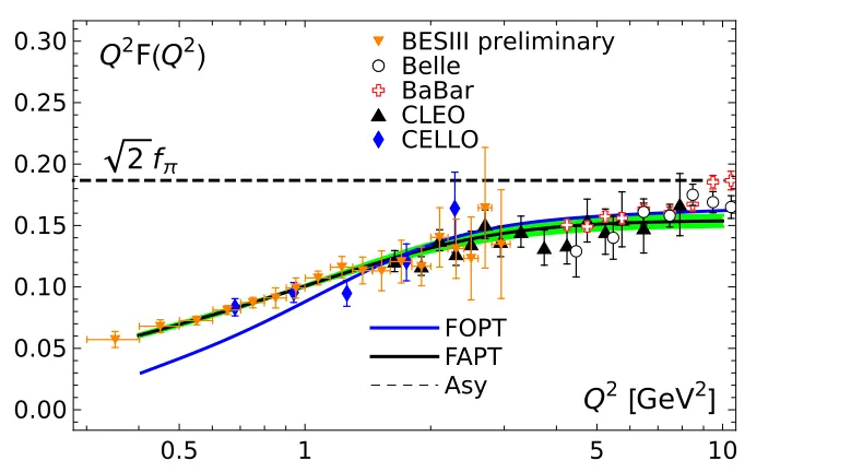
3.2 Numerical results for the TFF and comparison with the experimental data We show in Fig. 1 predictions for the TFF based on (19), obtained in two different approaches

to include the QCD radiative corrections using the LCSR method: 1) FAPT/LCSRs from Eq. (20)—black curve.

2) FOPT/LCSRs from the results in [2]—blue curve.

In both cases we employ the family of the bimodal BMS pion DAs obtained in [14]. For their parametrization it is sufficient to employ in the Gegenbauer decomposition (3a) the

coefficients{1,a2,a4}derived and discussed in [2, 14, 15]. The shown predictions are

cal-culated using the coefficient values at the normalization scaleµ2 _≈ 1 GeV2 _{[16, 17], viz.,} {a2(µ2)=0.20(+0.05/−0.06),a4(µ2)=−0.14(+0.09/−0.07), . . .}1. The other LCSR

param-eters have been fixed in previous investigations [1, 2] to bes0 ≈1.5 GeV2,M2 ≈0.9 GeV2, m2

ρ ≈ 0.6 GeV2,Λ₍₄₎(1−loop) ≈ 0.3 GeV ,δ2_tw-4(µ2) ≈ λq2/2 ≈ 0.19 GeV2 and are not varied here. On the other hand, the scale of the twist-six contribution in Eq. (22), for both used schemes FAPT/LCSRs and FOPT/LCSRs is fixed at the admissible upper limit of the

con-densateqq¯ 2 _=(0.25)6_GeV2_{, see, e.g., [13].}

Using Eq. (19) and the partial TFF terms Fγπ

LCSR;n from Eqs. (20), we obtain for

Q2_Fγπ

FAPT(Q2) the prediction shown by the solid black line for the BMS DA in Fig. 1. The

(green) strip enveloping this curve indicates the estimated range of theoretical variations of the BMS DA in terms ofa2anda4, while other uncertainties are not considered here. The

blue line in this figure corresponds to the FOPT predictionsQ2_Fγπ

FOPT(Q2) taken at the order

N2_LOβ

0within the LCSR scheme in [2]. Note that the radiative corrections are negative and

become too large in magnitude below about 1 GeV2_{. Obviously, the RG summation effect}

on the radiative corrections to the TFF provides a good agreement between the FAPT/LCSR

TFF predictions and the preliminary BESIII data [10] even in this very lowQ2_{domain, where}

FOPT turns out to be unreliable. This is remarkable, given that the experimental margin of error is very small in this range. The high-Q2 _{behavior of the TFF within the FAPT/LCSR}

approach will be considered elsewhere, while such predictions at the level N2_{LO within}

FOPT/LCSRs can be found in [11] with emphasis on the QCD asymptotic limit, denoted

in Fig. 1 by the dashed horizontal line.

In Eq. (20a) we have included in the zero-harmonic spectral density ¯ρ0 the contributions

stemming from the twist-four and twist-six terms. The latter term was first derived in [13] and reads

¯

ρ0(Q2,x) = ψ0(x)+

δ2_tw-4(Q2) Q2 x

d

dxϕ(4)(x)+ρ¯tw-6(Q2,x), (21)

ϕ(4)(x) = 80

3 x2(1−x)2;δ2tw-4(Q2)=  as(Q2₎

as(µ2₀)

 γtw-4β₀

δ2_tw-4(µ2₀), γtw-4=32/9,

¯

ρtw-6(Q2,x) = 8παsqq¯ 2

f2 π

CF

Nc

x Q4

[ −

( ₁

1−x )

+

+(2δ( ¯x)−4x)+x(3+2 ln(xx¯)) ]

.

Let us conclude this discussion by making two important remarks with regard to the TFF from the FAPT/LCSRs in (20): (i) Any N2LO contribution to Eqs. (20b), (20c) of orderO(A2+ν)

is expected to be sufficiently small due to the reason that_A2,A2are in the domainQ2 1

GeV2_{one order of magnitude smaller thanA}

1,A1[7]. (ii) For the numerical calculations of

the pion-photon TFF to follow, we replace theδ-model of the resonances in (20) with a more realistic Breit-Wigner model [1, 12].

3.2 Numerical results for the TFF and comparison with the experimental data We show in Fig. 1 predictions for the TFF based on (19), obtained in two different approaches

to include the QCD radiative corrections using the LCSR method: 1) FAPT/LCSRs from Eq. (20)—black curve.

2) FOPT/LCSRs from the results in [2]—blue curve.

In both cases we employ the family of the bimodal BMS pion DAs obtained in [14]. For their parametrization it is sufficient to employ in the Gegenbauer decomposition (3a) the

coefficients{1,a2,a4}derived and discussed in [2, 14, 15]. The shown predictions are

cal-culated using the coefficient values at the normalization scaleµ2 _≈ 1 GeV2 _{[16, 17], viz.,} {a2(µ2)=0.20(+0.05/−0.06),a4(µ2)=−0.14(+0.09/−0.07), . . .}1. The other LCSR

param-eters have been fixed in previous investigations [1, 2] to bes0 ≈1.5 GeV2,M2 ≈0.9 GeV2, m2

ρ ≈ 0.6 GeV2, Λ₍₄₎(1−loop) ≈ 0.3 GeV ,δ2_tw-4(µ2) ≈ λq2/2 ≈ 0.19 GeV2 and are not varied here. On the other hand, the scale of the twist-six contribution in Eq. (22), for both used schemes FAPT/LCSRs and FOPT/LCSRs is fixed at the admissible upper limit of the

con-densateqq¯ 2_=(0.25)6_GeV2_{, see, e.g., [13].}

Using Eq. (19) and the partial TFF terms Fγπ

LCSR;n from Eqs. (20), we obtain for

Q2_Fγπ

FAPT(Q2) the prediction shown by the solid black line for the BMS DA in Fig. 1. The

(green) strip enveloping this curve indicates the estimated range of theoretical variations of the BMS DA in terms ofa2anda4, while other uncertainties are not considered here. The

blue line in this figure corresponds to the FOPT predictionsQ2_Fγπ

FOPT(Q2) taken at the order

N2_LOβ

0within the LCSR scheme in [2]. Note that the radiative corrections are negative and

become too large in magnitude below about 1 GeV2_{. Obviously, the RG summation effect}

on the radiative corrections to the TFF provides a good agreement between the FAPT/LCSR

TFF predictions and the preliminary BESIII data [10] even in this very lowQ2_{domain, where}

FOPT turns out to be unreliable. This is remarkable, given that the experimental margin of error is very small in this range. The high-Q2 _{behavior of the TFF within the FAPT/LCSR}

approach will be considered elsewhere, while such predictions at the level N2_{LO within}

FOPT/LCSRs can be found in [11] with emphasis on the QCD asymptotic limit, denoted

in Fig. 1 by the dashed horizontal line.

1_{The valuesa2anda4are strongly correlated approximately along the linea2+a4=const.}

BESIII preliminary

Belle

BaBar

CLEO

CELLO

FOPT

FAPT

Asy

Q

F

(

Q

)

Q

[

GeV

]

2

f

0.5

1

5

10

0.00

0.05

0.10

0.15

0.20

0.25

0.30

Figure 1. The solid black line and the green strip around it are FAPT predictions forQ2_Fγπ

FAPT/LCSR,

whereas the blue line denotes the FOPT prediction forQ2_Fγπ

FOPT/LCSRat the N2LO. The experimental

data of different collaborations are shown in the upper part of the figure. The single fitted parameter is

the scale of the twist-six parameter fixed to the valueαsqq¯ 2defined at its upper boundqq¯ 2=(0.25)6

GeV2_.

4 Conclusion

We considered the lightcone sum-rule description of the pion-photon transition form fac-tor in combination with the renormalization group of QCD and compared the obtained TFF predictions with the corresponding fixed-order results. We showed that the LCSR method, augmented with the RG summation of radiative corrections, naturally leads to a version of fractional analytic perturbation theory that is free of Landau singularities and provides the possibility to include QCD radiative corrections in a resummed way [3]. This FAPT/LCSR

approach extends the domain of applicability of the QCD calculation well below 1 GeV2_and

amounts to a significantly smaller total contribution of radiative corrections in this regime relative to a fixed-order calculation. To ensure the compliance with the correct QCD asymp-totics of the form factor, new boundary conditions on the FAPT couplings at the origin,

Aν(Q2 = 0) = Aν(Q2 = 0) = 0,for 0 < ν 1, have to be imposed. The FAPT/LCSR

approach is best-suited for a detailed comparison with the expected final BESIII data that bear very small errors in the domain below 1 GeV2_{. In fact, as one sees from Fig. 1, the}

TFF calculated with the family of endpoint-suppressed BMS DAs [14], already agrees with the preliminary BESIII data very well. On the other hand, the TFF results for the BMS DAs within the FOPT/LCSR scheme agree with all data compatible with scaling at high-Q2values,

where radiative corrections can be reliably computed using FOPT [11].

Acknowledgments

References

[1] A. Khodjamirian, Eur. Phys. J.C6, 477 (1999),hep-ph/9712451

[2] S.V. Mikhailov, A.V. Pimikov, N.G. Stefanis, Phys. Rev. D93, 114018 (2016),

1604.06391

[3] C. Ayala, S.V. Mikhailov, N.G. Stefanis, Phys. Rev.D98, 096017 (2018),1806.07790 [4] A.V. Efremov, A.V. Radyushkin, Theor. Math. Phys.42, 97 (1980)

[5] G.P. Lepage, S.V. Brodsky, Phys. Rev.D22, 2157 (1980)

[6] A.P. Bakulev, S.V. Mikhailov, N.G. Stefanis, Phys. Rev.D72, 074014 (2005), [Erratum: Phys. Rev. D72, 119908 (2005)],hep-ph/0506311

[7] A.P. Bakulev, S.V. Mikhailov, N.G. Stefanis, Phys. Rev.D75, 056005 (2007), [Erratum: Phys. Rev. D77, 079901 (2008)],hep-ph/0607040

[8] A.P. Bakulev, Phys. Part. Nucl.40, 715 (2009),0805.0829 [9] N.G. Stefanis, Phys. Part. Nucl.44, 494 (2013),0902.4805

[10] C.F. Redmer (BESIII),Measurement of meson transition form factors at BESIII, in13th Conference on the Intersections of Particle and Nuclear Physics (CIPANP 2018) Palm Springs, California, USA, May 29-June 3, 2018(2018),1810.00654

[11] N.G. Stefanis, hep-ph/1904.02631

[12] S.V. Mikhailov, N.G. Stefanis, Nucl. Phys.B821, 291 (2009),0905.4004

[13] S.S. Agaev, V.M. Braun, N. Offen, F.A. Porkert, Phys. Rev. D83, 054020 (2011), 1012.4671

[14] A.P. Bakulev, S.V. Mikhailov, N.G. Stefanis, Phys. Lett.B508, 279 (2001), [Erratum: Phys. Lett. B590, 309 (2004)],hep-ph/0103119

[15] N.G. Stefanis, S.V. Mikhailov, A.V. Pimikov, Few Body Syst. 56, 295 (2015),

1411.0528

[16] A.P. Bakulev, S.V. Mikhailov, N.G. Stefanis, Phys. Rev. D67, 074012 (2003),

hep-ph/0212250

[17] A.P. Bakulev, S.V. Mikhailov, N.G. Stefanis, Annalen Phys. 13, 629 (2004),