Estimating Mutation Parameters, Population History and Genealogy Simultaneously From Temporally Spaced Sequence Data



Estimating Mutation Parameters, Population History and Genealogy

Simultaneously From Temporally Spaced Sequence Data

Alexei J. Drummond,*

_{Geoff K. Nicholls,}

_{Allen G. Rodrigo* and Wiremu Solomon}

*School of Biological Sciences,†_{Department of Mathematics and}‡_{Department of Statistics, University of Auckland 1001,} Auckland, New Zealand

Manuscript received December 15, 2001 Accepted for publication March 12, 2002

ABSTRACT

Molecular sequences obtained at different sampling times from populations of rapidly evolving pathogens and from ancient subfossil and fossil sources are increasingly available with modern sequencing technology. Here, we present a Bayesian statistical inference approach to the joint estimation of mutation rate and population size that incorporates the uncertainty in the genealogy of such temporally spaced sequences by using Markov chain Monte Carlo (MCMC) integration. The Kingman coalescent model is used to describe the time structure of the ancestral tree. We recover information about the unknown true ancestral coalescent tree, population size, and the overall mutation rate from temporally spaced data, that is, from nucleotide sequences gathered at different times, from different individuals, in an evolving haploid population. We briefly discuss the methodological implications and show what can be inferred, in various practically relevant states of prior knowledge. We develop extensions for exponentially growing population size and joint estimation of substitution model parameters. We illustrate some of the important features of this approach on a genealogy of HIV-1 envelope (env) partial sequences.

O

and Donnelly 2000), migration rates (Bahlo and

tion genetics modeling in recent times was the

Griffiths 2000), and recombination (Griffiths and

introduction ofcoalescentor genealogical methods (

King-Marjoram1996;FearnheadandDonnelly2001).

Me-man 1982a,b). The coalescent is a stochastic process

tropolis-Hastings Markov chain Monte Carlo (MCMC; that provides good approximations to the distribution

Metropoliset al.1953;Hastings1970) has been used of ancestral histories that arise from classical

forward-to obtain sample-based estimates of⌰ (Kuhner et al.

time models such as the Fisher-Wright (Fisher 1930;

1995), exponential growth rate (Kuhner et al.1998),

Wright1931) and Moran population models. The

ex-migration rates (BeerliandFelsenstein1999, 2001),

plicit use of genealogies to estimate population

parame-and recombination (Kuhneret al.2000).

ters allows the nonindependence of sampled sequences

In addition to developments in coalescent-based pop-to be accounted for. (“Genealogy” and “tree” are used

ulation genetic inference, sequence data sampled at interchangeably throughout. In both cases we are

refer-different times are now available from both rapidly ring to a collection of edges, nodes, and node times

evolving viruses, such as human immunodeficiency virus that together completely specify a rooted history.) Many

(HIV;Holmeset al.1992;Wolinskyet al.1996;Rodrigo

coalescent-based estimation methods focus on a single

et al.1999;Shankarappaet al.1999), and from ancient

genealogy (Fu1994;Neeet al.1995;Pybuset al.2000)

DNA sources (Hanniet al.1994; Leonardet al. 2000;

that is typically obtained using standard phylogenetic

Loreilleet al.2001;Barneset al.2002;Lambertet al.

methods. However, there is often considerable

uncer-2002). This temporally spaced data provides the poten-tainty in the reconstructed genealogy. To allow for this

tial to observe the accumulation of mutations over time uncertainty it is necessary to compute the average

likeli-and thus estimate mutation rate (Drummondand

Rod-hood of the population parameters of interest. The

cal-rigo2000;Rambaut2000). In fact, it is even possible

culation involves integrating over genealogies

distrib-to estimate variation in the mutation rate over time

uted according to the coalescent (Griffiths and

(Drummond et al. 2001). This leads naturally to the

Tavare 1994; Kuhner et al. 1995). We can carry out

more general problem of simultaneous estimation of this integration for some models of interest, using

population parameters and mutation parameters from Monte Carlo methods. Importance-sampling algorithms

temporally spaced sequence data (Rodrigoand

Felsen-have been developed to estimate the population

param-stein1999;Rodrigoet al.1999;Drummondand

Rod-rigo2000;Drummondet al.2001).

In this article we estimate population and mutation

1_{Corresponding author:Department of Statistics and Department of}

parameters, dates of divergence, and tree topology from Zoology, University of Oxford, South Parks Rd., Oxford, OX1 3PS,

United Kingdom. E-mail: [email protected] temporally spaced sequence data, using sample-based

Bayesian inference. The important novelties in the infer- and a second group of studies of synthetic sequence data.

ence are the data type (i.e., temporally sampled

se-Kingman coalescent with temporally offset leaves:In quences), the relatively large number of unknown model

this section we define the coalescent density for the parameters, and the MCMC sampling procedures, not

constant-sized Fisher-Wright population model. In

ex-the Bayesian framework itself. The coalescent gives ex-the

tensionswe give the corresponding density for the case expected frequency with which any particular genealogy

of a population with deterministic exponential growth. arises under the Fisher-Wright population model. The

It is assumed genealogies are realized by the Kingman coalescent may then be treated either as part of the

coalescent process. Our time units in this article are observation process defining the likelihood of

popula-“calendar units before the present” [e.g., days before

tion parameters or as the prior distribution for the

un-present (BP)], where the un-present is the time of the most known true genealogy. In either case we must integrate

recent leaf and set to zero. Let␳ denote the number

the likelihood over the state space of the coalescent.

of calendar units per generation and␪ ⫽Ne␳. The scale

Bayesian and purely likelihood-based population

ge-factor␪converts “coalescent time” to calendar time and

netic inference use the same reasoning and software up

is one of two key objects of our inference. Note that we to the point where prior distributions are given for the

do not estimate␳andNeseparately, only their product.

parameters of the coalescent and mutation processes.

Consider a rooted binary treegwithnleaf nodes and

Are there then any important difficulties or

advan-n ⫺ 1 ancestral nodes. For node i, let ti denote the

tages in a Bayesian approach over a purely

likelihood-age of that node in calendar units. Node labels are based approach? The principal advantage is the

possibil-numerically increasing with age soi⬎ jimpliestiⱖ tj.

ity of quantifying the impact of prior information on

LetIdenote the set of leaf node labels and letYdenote

parameter estimates and their uncertainties. The new

the set of ancestral node labels. There is one leaf node difficulty is to represent different states of prior

knowl-i僆Iassociated with each individual in the data. These

edge of the parameters of the coalescent and mutation

individuals are selected, possibly at different times, from processes as probability densities. However, such prior

a large background population. An edge具i,j典,i⬎ jof

elicitation is often instructive. In the absence of prior

grepresents an ancestral lineage. Going back in time,

information, researchers frequently choose to use

non-an non-ancestral nodei 僆Ycorresponds to acoalescenceof

informative/improper priors for the parameters of

in-two ancestral lineages. The root node, with label i ⫽

terest. Such an approach may be problematic and can

2n ⫺ 1, represents the most recent common ancestor

result in improper posterior distributions. There exist

(MRCA) of all leaves. LettIbe the times of the leaves

a number of important cases in the literature in which

andtYbe the divergence times of the ancestral nodes.

knowledgeable authors inadvertently analyze a

mean-Let Eg denote the edge set of g, so that g ⫽ (Eg, tY)

ingless, improper posterior distribution. Why then do

specifies a realization of the coalescent process. For we choose to treat improper priors in this article? We

givenn and tI, let⌫ denote the class of all coalescent

are developing and testing inferential and sampling

trees (Eg,tY) withnleaf nodes having fixed agestI.The

methods. These methods become more difficult as the

agestYare subject to the obvious parent-child age order

amount of information in the prior is reduced. The

constraint. The element of measure in⌫ isdg ⫽dtn⫹1

sampling problem becomes significantly more difficult.

. . .dt2n⫺1with counting measure over distinct topologies

We therefore treat the “worst case” prior that might

associated with the distinguishable leaves. naturally arise. Since this prior is improper, we are

The probability density for a tree, fG(g|␪), g 僆 ⌫ is

obliged to check that the posterior is proper. However,

computed as follows. Letkidenote the number of

lin-when confronted with a specific analysis, detailed

bio-eages present in the interval of time between the node logical knowledge should be encoded in the prior

distri-i⫺1 and the nodei.The coalescent process generates

butions wherever possible.

g⫽(Eg,tY) with probability density

Although Bayesian reasoning has frequently been

ap-plied to phylogenetic inference (Yang and Rannala

fG(g|␪)⫽

1

␪n⫺1·

兿

i⫽2

e(⫺k_i(ki⫺1)/2␪)(ti⫺t_i⫺1)_{. (1)}

1997;Thorneet al.1998;Mauet al.1999;Huelsenbeck

et al.2000), it has thus far been the exception in

popula-tion genetic inference (WilsonandBalding1998). The interpretation is as follows. Fix a timetand suppose

In this article, we begin with a description of the mod- klineages are present at that time. A coalescence event

els we use. We then give the overall structure of the between any of the k(k⫺ 1)/2 pairs of distinguished

inferential framework, followed by an overview of how lineages occurs at instantaneous rate 1/␪. Given that

MCMC is carried out. We mention extensions of the two lineages coalesce at time t, the probability it was

basic inference that allow for (1) deterministically vary- some particular pair is 2/k(k ⫺ 1). It follows that, in

ing populations and (2) estimation of substitution pa- the time interval of lengthti ⫺ti⫺1preceding the time

rameters. Finally, we illustrate our methods with a group of a leaf nodei僆I, “nothing” happens with probability

e(⫺ki(ki⫺1)/2␪)(ti⫺ti⫺1) _{and that the length of time, t} ⫺ _t

i⫺1,

preceding coalescent nodei僆 Yis a random variable ofR.We return to inference for relative rates in exten-sions.

with density (ki(ki ⫺ 1)/2␪) · e(⫺ki(ki⫺1)/2␪)(ti⫺ti⫺1). Taking

the product of these factors over all intervals [ti⫺1, ti], We now write the likelihood for␮. Consider an edge

具i,j典僆Egof treeg.The individual associated with node

i⫽ 2, 3, . . . , 2n⫺1, we obtain Equation 1 (Rodrigo

andFelsenstein1999). jis a direct descendant of the individual associated with

node i. However, the sequences Di and Dj may differ

Mutation: We use the standard finite-sites

selection-neutral likelihood framework (Felsenstein1981) with if mutations have occurred in the interval. Let eQ

de-note the 4 ⫻ 4 matrix exponential of Q.In the

stan-a generstan-al time-reversible (GTR) substitution model

(Rodriguezet al.1990). However, as we are considering dard finite-sites selection-neutral likelihood framework Pr{Dj,s⫽c⬘|Di,s⫽c}⫽[e⫺Q␮(ti⫺tj)]c,c⬘forc僆C. The

proba-genealogies in calendar units (or generations) as

op-posed to mutations we take some space to develop nota- bility for any particular set of sequences D, DA to be

realized at the nodes of a given tree is tion.

Associated with each leaf nodei僆Ithere is a

nucleo-Pr

兵

其

兿

具i,j典僆Eg

兿

L

s⫽1

Dj,s⬆φ

[eQ␮(t_i⫺t_j)_]

Di,s,Dj,s (4)

tide sequenceDi⫽(Di,1,Di,2, . . . ,Di,s, . . . ,Di,L) of some

fixed lengthL, say. Nucleotide base charactersDi,s,i僆

I,s⫽1, 2, . . . ,Ltake values in the setC⫽ {A, C, G,

(in the above formula, compact notation is obtained by

T }. An additional gap character, φ, indicates missing

including in the product over edges an edge terminating

data. LetD⫽(D1,D2, . . . ,Dn)Tdenote then⫻Lmatrix

at the root from an ancestor of infinite age). We may

of sequences associated with the tree leaves, and letDA

eliminate the unknown ancestral sequencesDAfrom the

denote the (n⫺1)⫻Lmatrix of unknown sequences

above expression by simply summing allDA 僆D,

associated with the ancestral nodes. The data are D

together withtI, that is, thensequences observed in the

Pr

兵

其

兺

DA僆D

Pr

兵

其

leaf individuals and thenages at which those individual

sequences were taken. Let D ⫽ C(n⫺1)L _{denote the set}

It is feasible to evaluate this sum, using a pruning

algo-of all possible ancestral sequences. Consider a sites⫽

rithm (Felsenstein1981).

1, 2, . . . ,Lin the nucleotide sequence of an individual.

Bayesian inference for scale parameters:We now

con-The character at sitesmutates in forward time according

sider Bayesian inference for scale parameters␮and␪.

to a Poisson jump process with 4 ⫻ 4 rate matrix Q.

Both of these quantities take a real positive value. The

Here, Qi,j is the instantaneous rate for the transition

joint posterior density, hM⌰G(␮, ␪, g|D), for the scale

from character i to character j, and A ←1, C ← 2,

parameters and genealogy, is given in terms of the

likeli-G←3, T ←4. We assume mutations are independent

hood and coalescent densities above and two additional

between sites. Let␲ ⫽(␲A,␲C,␲G,␲T) be a 1⫻4 vector

densities, fM(␮) and f⌰(␪). These functions quantify

of base frequencies, corresponding to the stationary

prior information about the scale parameters. LetZbe

distribution of the mutation process,␲Q⫽(0, 0, 0, 0).

an unknown normalizing constant. The posterior is then

The matrixQis parameterized in terms of a symmetric

“relative rate” matrixR,

hM␪G(␮,␪,g|D)⫽

1

ZPr

兵

其

We are interested in the marginal density,hM⌰(␮,␪|D).

R⫽     

RA↔C RA↔G RA↔T RA↔C RC↔G RC↔T RA↔G RC↔G 1 RA↔T RC↔T 1

     (2)

We summarize this density using samples (␮, ␪, g)ⵑ

hM⌰G. The sampled genealogies can be thought of as

uninteresting “missing data.” as

Consider now the densities fM(␮) and f⌰(␪). In any

particular application these functions will be chosen to

Qi,j⫽

␲iRi,j

兺

兺

, i⬆j

summarize available prior knowledge of scale parame-ters. It is common practice to avoid the problem of prior

Qi,j⫽ ⫺

兺

elicitation and attempt to construct a “noninformative” prior. This notion is poorly defined, since a prior may

The time units of the rateQi,jhave been chosen so that

the mean number of mutations per unit time occurring be noninformative with respect to some hypotheses,

but informative with respect to others. Nevertheless, we

at a site is equal to one. Let␮give the mean number

of mutations per calendar unit (e.g., mutations per year) illustrate sample-based Bayesian inference under a prior

that contains little information. We do this for two rea-at a site.

The conversion factor ␮ is the second of the two sons. First, we wish to give our sampling instruments a

thorough workout. From this point of view an improper

principal objects of our inference. In addition to␮, the

relative rates,R, may be estimated. We have found that prior is the best choice. Second, when carrying out

Bayesian inference, it is necessary to test the sensitivity of wherever it is feasible to estimate the scale parameters

What conclusions would a person in a state close to ignorance reach from these data? The improper prior we consider represents ignorance of a rather natural kind. People using our methods will very likely want to consider this particular state of knowledge, along with others that are more representative of their own.

In our case ␮ and␪ are both scale parameters (for

time). The Jeffreys prior, f(z) ⬀ 1/z, z ⬎ 0, invariant

under scale transformations z → az, and the uniform

prior on z ⬎ 0 are candidates for fM(␮) and f⌰(␪). If

fM ⬀ 1/␮, f⌰ ⬀ 1/␪, and fG(g|␪) and Pr{D|g, ␮} are as

given in Equations 1 and 5 then it may be shown that the posterior density in Equation 6 is not finitely normal-izable. We may nevertheless consider ratios of posterior densities. But that means the only feasible Bayesian in-ference, at least under the uniform, improper prior, is exactly frequentist inference. We cannot treat the parameters of interest as random variables. Suppose

fixed upper limits ␮ ⱕ ␮* and troot ⱕ t*root may be set, _{Figure1.—Diagrams of two proposal mechanisms used to}

along with a lower limit ␪ ⱖ ␪*. For the problems we _{modify tree topology during an MCMC analysis. (A) This move}

use to illustrate our methods inexamples, conservative is called the “narrow exchange” and is similar to a nearest

neighbor interchange. This move picks two subtrees at

ran-limits of this kind determine a state of knowledge that

dom under the constraint that they have an aunt-niece

rela-arises quite naturally. Moreover it may be shown that the

tionship; i.e., the parent of one is the grandparent of the

posterior density is finitely normalizable under uniform _{other, but neither is parent of the other. Once picked these}

priors on the restricted state space, even though the _{two subtrees are swapped so long as doing so does not require}

prior on␪ remains improper. any modifications in node heights to maintain parent-child

order constraints. (B) This move is similar to one proposed

by Wilson and Balding (1998) and involves removing a

subtree and reattaching it on a new parent branch. MARKOV CHAIN MONTE CARLO FOR

EVOLUTIONARY PARAMETERS

The posterior densityhM⌰Gis a complicated function dard deviation of some estimate of␳f(k), formed from

defined on a space of high dimension (between 30 and the MCMC output. Large lag autocorrelations should

40 in the examples that follow). We summarize the fall off to zero and remain withinO(␥f) of zero, as

dis-information it contains by computing the expectations, cussed by Geyer (1992). Note that in the examples

overhM⌰G, of various statistics of interest. These expecta- section, these standards are not uniformly applied. The

tions are estimated using samples distributed according first two analyses pass all three checks. The last two

tohM⌰G. We use MCMC to gather the samples we need. analyses pass the first test. Here we are displaying the

MCMC and importance sampling are part of a family limitations of our MCMC algorithm. However, we

be-of Monte Carlo methods that may be used individually lieve the convergence is adequate for the points we

or in concert to solve the difficult integration problems make. In the appendix,Convergence and standard errors

that arise in population genetic inference. Earlier work describes the integrated autocorrelation time (IACT)

on this subject is cited in the Introduction. Figure 1 and effective sample size (ESS) measures used to test

shows a cartoon of two proposal mechanisms used. See the efficiency of our sampler.

the appendix for details of the proposal mechanisms The MCMC algorithm we used was implemented

and MCMC integration performed. twice, more or less independently, by A. Drummond,

As always in MCMC, it is not feasible to test for conver- in JAVA and by G. K. Nicholls in MatLab. This allowed us

gence to equilibrium. MCMC users are obliged to test to compare results and proved very useful in debugging

for stationarity as a proxy. We make three basic tests. some of the more complex proposal mechanism

combi-First, we check that results are independent of the start- nations. To minimize programming burden, one of our

ing state using 10 independent runs with very widely implementations (G. K. Nicholls in MatLab) was partial,

dispersed initializations. Second, we visually inspect out- allowing only fixed population size and fixed Rto be

put traces. These should contain no obvious trend. compared. This is discussed more extensively in

Imple-Third, we check that the MCMC output contains a large mentation issuesin theappendix.

number of segments that are effectively independent of one another, independent, at least, in the distribution

EXTENSIONS

determined empirically by the MCMC output. Let␳f(k)

give the autocorrelation at lagkfor some functionfof Extending the framework of the Introduction and

MCMC for evolutionary parametersto include

stan-terministically varying models of population history and study. The total dataset consists of 60 sequences from these five time points. The length of the alignment is estimation of relative rate parameters is straightforward.

Let⌽ ⫽(0,∞)5_{be the state space for the relative rates 660 nucleotides. Gapped columns were included in the}

analysis. The evidence for recombination seems to be

of Rabove the diagonal and excluding RG↔T. Let s ⫽

(␮,␪,g,r,R), and lethS(s|D) denote the posterior density negligible in this dataset (Rodrigo et al. 1999) and

recombination is ignored for the purposes of illustrating

forS僆⍀*S, where⍀*S ⫽ ⍀*M⌰G⫻ᑬ ⫻ ⌽(see the

appen-dix). The posterior probability density has the form our method. Rough estimates ofNemay be obtained by

assuming a generation length of␳ ⫽1 day per

genera-tion (Rodrigoet al.1999). However, we emphasize that

hS(s|D)⫽

1

ZPr

兵

其

(7) _{into two subsets for separate analysis. One contained all}

pretreatment sequences (28 sequences), and the other

LetTdenote the age of the most recent leaf,i.e.,T⫽

contained all sequences after treatment commenced

mini僆Iti. In this article T ⫽ 0. Let t ⱖ T be a generic

(32 sequences; henceforth called posttreatment). The

age. In this modelNe⫽Ne(t). Recall that␳, the number

rationale behind this split is that both (1) population of calendar units per generation, is an unknown

con-size and (2) mutation rate per unit time may be affected

stant. Define a constant␪ ⫽Ne(T)␳and a growth rate

by a replication inhibitor such as Ziduvodine. In all of

parameterr. The densityfG(g|␪,r) is the density

deter-the analyses, base frequencies were fixed to empirically mined by the coalescent process with a population

grow-determined values; however, inference of these would

ing as Ne(t) ⫽ (␪/␳)e⫺r(t⫺T) (Slatkin and Hudson

have been trivial. Two analyses are undertaken on each

1991). In terms of the notation defined in Kingman

dataset. The pretreatment data are strongly informative

coalescent with temporally offset leavesin connection with

for all parameters estimated. The results are robust to Equation 1, for genealogies with temporally spaced tips

the choice of priors and MCMC convergence is quick. the density is

In contrast, the posttreatment data are only weakly

infor-mative for ␮, ␪, and troot parameters; the results are

fG(g|␪,r)⫽

1

␪n⫺1·

兿

i⫽2

ert_ie(⫺k_i(k_i⫺1)/2␪r)(erti⫺erti⫺1)_{. (8)}

sensitive to the choice of prior; and MCMC convergence is very slow.

If all of the relative rates inR, exceptRG↔T, are estimated _{Pretreatment data, constant population size, HKY}

substitu-we are fitting a general time-reversible model of substitu- _{tion: In this first analysis of the pretreatment dataset,}

tion. However, it is sometimes useful to consider simpler _{we fit the HKY substitution model and assume a constant}

nested models. One such model is the Hasegawa-Kis- _{population size. We are estimating␮,␪,g, and ␬. We}

hino-Yano (HKY) model (Hasegawa et al. 1985). In _{illustrate our methods using uniform prior distributions}

the HKY model transitions occur at rate ␬ relative to _{on␮and ␪, an upper limit on mutation rate of␮* ⫽}

transversions. ThusRA↔G⫽RC↔T⫽ ␬andRA↔C⫽RA↔T⫽ _{1, a lower limit onN}e␳_of␪_*⫽_{1, and a very conservative}

RC↔G⫽ RG↔T ⫽ 1. Either a Jeffreys prior or a uniform _{upper limit ont}

root oft* ⫽ 107 days. Ten MCMC runs

prior can be used for the relative rates. However, as a _{were made, with starting values for mutation rate}

distrib-result of our parameterization, the Jeffreys prior pro- _{uted on a log scale from 5⫻10}⫺3_{down to 10}⫺7

muta-vides more accurate estimates. In the examples that _{tions/site/day. This range greatly exceeds the range}

follow, a uniform prior is used forRand␬as this repre- _{of values supported by the posterior. To test MCMC}

sents the most ignorant state of knowledge and is more _{convergence on tree topologies, each of the 10 MCMC}

than adequate for the purpose of illustrating the meth- _{runs was started on a random tree drawn from a}

coales-odology. In the same spiritfr(r) is set uniform onr, and _{cent distribution with population size equal to 1000 (in}

this also proves acceptable. _{exploratory work we initialize on a sUPGMA or}

neigh-bor-joining topology). The 10 Markov chain simulations were run for 2,000,000 steps and the first 100,000 steps

EXAMPLES

were discarded as burn-in. Each run tookⵑ4 hr on a

machine with a 700 MHz Pentium III processor. The In this section, we illustrate our methods on two HIV-1

envdata sets and a series of synthetic data sets of compa- mean IACT of the mutation rate parameter was 4190,

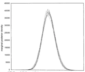
giving an ESS ofⵑ450 per simulation. Table 1 presents

rable size.

HIV-1envdata:The method was first tested on HIV-1 parameter estimates for all 10 runs, illustrating close concordance between runs. Note also that the variabil-partial envelope sequences obtained from a single

pa-tient over five sampling occasions spanning ⵑ3 years: ity, between runs, of estimated means is in line with

standard errors estimated within runs. This is a consis-an initial sample (day 0) followed by additional samples

after 214, 671, 699, and 1005 days. Details of this dataset tency check on our estimation of the IACT. Figures 2

and 3 show the marginal posterior density of␮and␪

have been published previously (Rodrigoet al.1999).

An important feature of these data is that monotherapy for each of the 10 runs. In all 10 runs the consensus

tree computed from the MCMC output was the same,

with Zidovudine was initiated on day 409 (Drummond

ran-TABLE 1

Parameter estimates for 10 independent analyses of the pretreatment dataset assuming constant population size and HKY model of mutation

Mutation rate Population size

(mutations/generation/site ⫻generation Age of root Transition/transversion Run ⫻105_{) length (}␪_{) (days) bias parameter (}␬₎

1 6.238 (0.0517)a _{1284 (13.0) 796 (6.03) 4.132 (0.00634)}

2 6.173 (0.0498) 1304 (12.7) 799 (5.99) 4.141 (0.00599) 3 6.218 (0.0466) 1291 (12.7) 794 (5.45) 4.124 (0.00631) 4 6.168 (0.0434) 1303 (14.0) 797 (5.65) 4.138 (0.00629) 5 6.297 (0.0474) 1269 (12.8) 784 (5.45) 4.134 (0.00640) 6 6.159 (0.0458) 1309 (12.4) 802 (6.21) 4.135 (0.00630) 7 6.308 (0.0539) 1270 (13.9) 784 (5.90) 4.130 (0.00678) 8 6.256 (0.0463) 1279 (11.5) 790 (5.63) 4.133 (0.00674) 9 6.247 (0.0474) 1283 (13.1) 791 (5.75) 4.122 (0.00661) 10 6.201 (0.0578) 1291 (15.4) 801 (7.54) 4.123 (0.00736)

Overall 6.227 1288 794 4.131

95% HPD interval [4.20, 8.28] [660, 2050] [580, 1040] [3.07, 5.31]

a_{Numbers in parentheses are the standard errors of the means calculated using IACT statistic.}

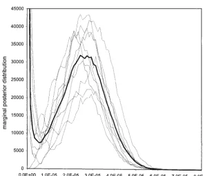
domly (data not shown). Combining the output of all independent runs of 3,000,000 cycles, each starting with

an independent random tree topology (the mean IACT 10 runs, the 95% highest posterior density (HPD)

inter-vals for the mutation rate andtrootare, respectively, [4.20, for␮was 7955 giving an ESS of 358 per run). Figure 4

shows the 10 estimates of the marginal posterior density

8.28]⫻10⫺5_{mutations per site per day, and [580, 1040]}

days. of mutation rate. Table 2 shows parameter estimates for

each of the 10 runs. Convergence is still achieved with

Pretreatment data, exponential growth, general substitution

model:In this second analysis of the pretreatment data- the extra parameters.

Compare the distribution of summary statistics under set, we fit the general time-reversible substitution model,

with exponential growth of population size. We are esti- the two models described here and inPretreatment data,

constant population size, HKY substitution. Given the na-mating␮,␪,g,r,RA↔C,RA↔G,RA↔T,RC↔G, andRC↔T. This

is the most parameter-rich model we fit. To assess the ture of infection of HIV-1, it seems likely that an

expo-nential growth rate assumption is more accurate. Esti-convergence characteristics of this analysis we ran 10

Figure2.—The marginal posterior density of

Figure3.—The marginal posterior density of

␪for 10 independent MCMC runs on the pretreat-ment HIV-1envdataset. Each run was started on a random tree topology. Initial mutation rates ranged from 5e-3 to 1e-7.

mated 95% HPD intervals for the growth rater, [1.09⫻ population size. The first analysis uses the same priors

as the first pretreatment analysis. In contrast to the

10⫺3_{, 6.65}⫻₁₀⫺3_{], exclude small growth rates,}

corrobo-rating this view. The 95% HPD intervals for the mutation pretreatment dataset, the mutation rate of the

posttreat-ment dataset is difficult to estimate. This is illustrated

rate andtrootare, respectively, [3.61, 8.11]⫻10⫺5

muta-tions per site per day and [570, 1090] days. Compare in Figures 5 and 6, in which the marginal posterior

densities of ␮ and ␪ estimated from 10 independent

these with the model inPretreatment data, constant

popula-tion, HKY substitution. The change in model has minimal MCMC runs, each 5,000,000 cycles long, are compared. We were unable to compute an IACT for each run,

effect (⬍10%) on the posterior mean mutation rate.

Posttreatment: The posttreatment data are analyzed so we are unable to compare within- and between-run variability. However, the between-run concordance visi-twice under the HKY substitution model with constant

Figure4.—The marginal posterior density of

TABLE 2

Parameter estimates for 10 independent analyses of the pretreatment dataset assuming exponential growth and GTR model of mutation

Mutation rate Population size

(mutations/generation/site ⫻generation Age of root Growth rate

Run ⫻105_{) length (}␪_{) (days) (r}⫻₁₀3₎

1 5.910 (0.0623)a _{5404 (127) 800 (7.43) 3.815 (0.0407)}

2 5.761 (0.0526) 5321 (125) 821 (7.05) 3.719 (0.0436) 3 6.045 (0.0550) 5089 (123) 786 (6.85) 3.832 (0.0418) 4 5.891 (0.0708) 5443 (172) 806 (8.56) 3.839 (0.0377) 5 5.849 (0.0609) 5338 (113) 812 (8.05) 3.815 (0.0423) 6 5.930 (0.0615) 5242 (170) 804 (8.66) 3.748 (0.0409) 7 5.857 (0.0589) 5318 (148) 806 (7.33) 3.780 (0.0388) 8 5.809 (0.0605) 5236 (123) 817 (7.51) 3.696 (0.0382) 9 5.982 (0.0542) 5064 (127) 795 (5.63) 3.786 (0.0382) 10 5.859 (0.0692) 5306 (188) 813 (10.2) 3.708 (0.0400)

Overall 5.889 5276 806 3.774

95% HPD interval [3.61, 8.11] [920, 12450] [570, 1090] [1.09, 6.65]

a_{Numbers in parentheses are the standard errors of the means calculated using IACT statistic.}

ble in Figure 5 justifies the following statement. The of low␮and largetrootare not well distinguished from

otherwise identical states of larger␮and smallertroot.

posttreatment mutation rate shows one mode atⵑ2.8⫻

10⫺5 _{mutations/site/day with a second mode on the In the second posttreatment analysis, we revise the}

upper limit ontrootdownwards, from 107to t* ⫽3650,

lower boundary. The data determine a diffuse, and

bi-modal, marginal posterior on ␮. One of the modes is a value more representative of actual prior knowledge

for this dataset. The new limit, set 3 years before

sero-associated with states (␮,␪,g) with physically unrealistic

root times (greater than the age of the patient). These conversion occurred in the infected patient, is still

con-servative. Here we explored the prior belief that HIV are allowed, if we are not prepared to assert some

restric-tion on troot. This behavior also occurs when we use a infection most often originates from a small,

homoge-nous population and then subsequently accumulates Jeffreys prior on the mutation rate (data not shown).

It reflects a real property of the data, namely that states variation. This prior effectively assumes that all viruses

Figure5.—The marginal posterior density of

Figure6.—The marginal posterior density of

␪for 10 independent MCMC runs on the post-treatment HIV-1envdataset. Each run was started on a random tree topology. Initial mutation rates ranged from 5e-3 to 1e-7.

in an infected individual share a common ancestor at 5 and 6. Information abouttroothas been converted into

information about mutation rates and population size. most as old as the time of infection of the host. The

estimated 95% HPD interval for the mutation rate was Simulated sequence data: To test the ability of our

inference procedure to recover accurate estimates of

[1.16, 4.27]⫻10⫺5_{mutations/site/day, markedly down}

from the pretreatment mutation rate. Figure 7 depicts parameters from the above HIV-1 dataset we undertook

four simulation studies. In each experiment we gener-the resulting unimodal marginal posterior density for

mutation rate, showing that the spurious mode has been ated 100 synthetic datasets. For experiment 1, the

poste-rior estimates of␪,␮, and␬obtained from the

pretreat-eliminated. Again, no IACT was computed. However,

between-run variability was much improved over Figures ment dataset inPretreatment data, constant population size,

Figure7.—The marginal posterior density of

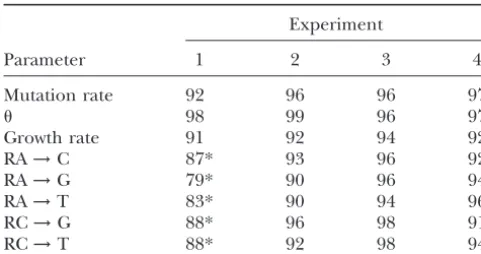
TABLE 3 ments 3 and 4 demonstrate that the use of a Jeffreys prior for these and other scale parameters results in Percentage of times that the true parameter was found in the

⬎90% recovery in all parameters. We are not aiming

95% HPD region of the marginal posterior density

to prescribe any particular noninformative prior. Our choice of uniform prior in earlier experiments is

delib-Experiment

erately crude. However, it allows us to lay out the

meth-Parameter 1 2 3 4

odology with as little emphasis as possible on prior

elic-Mutation rate 92 96 96 97 itation. The reader should undertake this process for a

␪ 98 99 96 97 _{specific problem.}

Growth rate 91 92 94 92

RA→C 87* 93 96 92

RA→G 79* 90 96 94 DISCUSSION

RA→T 83* 90 94 96

We have described Bayesian coalescent-based

meth-RC→G 88* 96 98 91

ods to estimate and assess the uncertainty in mutation

RC→T 88* 92 98 94

parameters, population parameters, tree topology, and

*Success rate was significantly⬍95%.

dates of divergence from aligned temporally spaced se-quence data. The sample-based Bayesian framework allows us to bring together information of different

HKY substitution were used to generate 100 coalescent _{kinds to reduce uncertainty in the objects of the}

infer-trees and then simulate sequences on each of the re- _{ence. Much of the hard work is in designing,}

implement-sulting trees. The synthetic data were generated under a _{ing, and testing a suitable Monte Carlo algorithm. We}

constant-size population model with the HKY mutation _{found a suite of MCMC updates that do the job.}

model but analyzed under an exponentially growing _{We have analyzed two contrasting HIV-1 datasets and}

population model and a GTR mutation model. In the _{400 synthetic datasets to illustrate the main features of}

second experiment, 100 synthetic datasets were gener- _{our methods. The results of the three HIV-1 env data}

ated using the pretreatment parameter estimates inPre- _{subsections show that a robust summary of}

parameter-treatment data, exponential growth, general substitution model _{rich models, including the joint estimation of mutation}

as the true values. In this case the models for simulation _{rate and population size, is possible for some}

moderate-and inference are matched. Synthetic data were gener- _{sized datasets. The pretreatment data restrict the set}

ated under an exponentially growing population model _{of plausible parameter values to a comparatively small}

and a GTR mutation model. In both experiments 1 and _{range. For this dataset, useful results can be obtained}

2 uniform bounded priors were used for all parameters. _{from a state of ignorance about physically plausible}

out-Experiments 3 and 4 differed from experiments 1 and _{comes. This situation is in contrast to the situation}

illus-2 only in that we usedJeffreys’(1946) prior for scale _{trated in thePosttreatmentsection. For this dataset, prior}

parameters (mutation rate, population size, and relative _{ignorance implies posterior ambiguity, in the form of}

rates). _{a bimodal posterior distribution for the mutation rate.}

All datasets had the same number of sequences (28), _{One of these modes is supported by genealogies}

con-the same sampling times (0 and 214 days), and con-the same _{flicting with very basic current ideas about HIV}

popula-sequence length (660) as the pretreatment dataset. Ta- _{tion dynamics. We modify the coalescent prior on}

gene-ble 3 shows that the true values are successfully recov- _{alogies to account for this prior knowledge, restricting}

ered (i.e., fall within the 95% HPD interval)ⱖ90% of the _{the most recent common ancestor to physically realistic}

time in all cases except for the relative rate parameters in _{values. The ambiguity in mutation rate is removed.}

Simi-experiment 1. In the most complex model we fit, we _{lar results could be obtained in a likelihood-based}

analy-recover true parameter values. The overparameteriza- sis of the posttreatment data, since the prior information

tion present in experiments 1 and 3 does not seem amounts to an additional hard constraint on the root

problematic for estimating mutation rate,␪, or growth time of the coalescent genealogy.

rate. These results suggest that inference of biologically There is some redundancy in the set of MCMC

up-realistic growth rates is quite feasible. The relative rates dates we used, in the sense that the limiting distribution

performed most poorly in the parameters of interest. of the MCMC is unaltered if we remove the scaling

This is caused predominantly because the uniform prior update (move 1) or the Wilson-Balding update (move

on relative rates introduces metric factors that inflate 2; see appendixfor details of these moves). However,

the densities. In experiment 1, when the true value of these two updates types are needed in practice. There

a relative rate parameter was not within the 95% HPD are two timescales in MCMC, time to equilibrium and

interval (which occurred 75 times out of 500), it was mixing time in equilibrium. The scaling move sharply

almost always overestimated (74 out of 75 times). Fur- reduces mixing time in equilibrium. The

Wilson-Bald-thermore, conditioning on a tranversion (RG↔T⫽1), a ing update is needed to bring the equilibrium time to

experi-minus the Wilson-Balding move, in which an apparently LITERATURE CITED

stationary Monte Carlo process undergoes a sudden and _{Bahlo, M.,andR. C. Griffiths,2000 Inference from gene trees}

unheralded mean shift at ⵑ2,000,000 updates. This in a subdivided population. Theor. Popul. Biol.57:79–95.

Barnes, I., P. Matheus, B. Shapiro, D. JensenandA. Cooper,2002 problem was picked up at the debugging stage, in

com-Dynamics of Pleistocene population extinctions in Beringian

parisons between our two MCMC implementations. Sub- _{brown bears. Science295:2267–2270.}

sequent simulation has shown that the genealogies ex- Beerli, P.,andJ. Felsenstein,1999 Maximum-likelihood

estima-tion of migraestima-tion rates and effective populaestima-tion numbers in two plored in the first 2,000,000 updates of that simulation

populations using a coalescent approach. Genetics152:763–773.

were just one of the tree clusters supported by the target _{Beerli, P.,andJ. Felsenstein,2001 Maximum likelihood}

estima-distribution. tion of a migration matrix and effective population sizes in

sub-populations by using a coalescent approach. Proc. Natl. Acad. The methods presented here reduce to those of

Sci. USA98:4563–4568.

Felsenstein and co-workers (Kuhneret al.1995) in the _{Drummond, A.,andA. G. Rodrigo,2000 Reconstructing}

genealo-case of a uniform prior on⌰ ⫽2Ne␮, a fixedR, a fixed␮, gies of serial samples under the assumption of a molecular clock

using serial-sample UPGMA. Mol. Biol. Evol.17:1807–1815. and contemporaneous data, if instead of summarizing

Drummond, A.,and K. Strimmer, 2001 PAL: an object-oriented results using 95% HPD interval estimates, we use the

programming library for molecular evolution and phylogenetics.

mode and curvature of the posterior density for⌰ to _{Bioinformatics17:662–663.}

Drummond, A., R. ForsbergandA. G. Rodrigo,2001 The infer-recover the maximum-likelihood estimate (MLE) and

ence of stepwise changes in substitution rates using serial se-its associated confidence interval.

quence samples. Mol. Biol. Evol.18:1365–1371.

A distinction can be made between a dataset, like the _{Fearnhead, P.,andP. Donnelly,2001 Estimating recombination}

pretreatment dataset, for which there is strong statistical rates from population genetic data. Genetics159:1299–1318.

Felsenstein, J.,1981 Evolutionary trees from DNA sequences: a information about mutation rates (we refer to

popula-maximum likelihood approach. J. Mol. Evol.17:368–376.

tions from which such datasets may be obtained as “mea- _{Fisher, R. A.,1930 The Genetical Theory of Natural Selection.Clarendon}

surably evolving”), and a dataset, like the posttreatment Press, Oxford.

Fu, Y. X.,1994 A phylogenetic estimator of effective population size data, in which the statistical signal is weak. In both of

or mutation rate. Genetics136:685–692.

these datasets the familiar parameter ⌰ ⫽ 2Ne␮ is in _{Geyer, C. J.,1992 Practical Markov chain Monte Carlo. Stat. Sci.7:}

fact well determined by the data (not shown above), so 473–511.

Green, P. J.,1995 Reversible jump Markov chain Monte Carlo

com-that MCMC convergence in⌰ is quick. However, it is

putation and Bayesian model determination. Biometrika82:711– only in the pretreatment data that this parameter can

732.

be separated easily into its two factors. This is related to _{Griffiths, R. C.,andP. Marjoram,1996 Ancestral inference from}

samples of DNA sequences with recombination. J. Comput. Biol. the well-known problem of identifiability for population

3:479–502. size and mutation rate. We can see that temporally

Griffiths, R. C.,andS. Tavare,1994 Ancestral inference in

popula-spaced data may or may not contain information that _{tion genetics. Stat. Sci.9:307–319.}

allows us to separate these two factors. In this particular Hanni, C., V. Laudet, D. StehelinandP. Taberlet,1994 Tracking

the origins of the cave bear (Ursus spelaeus) by mitochondrial example, lineages of the posttreatment viruses branch

DNA sequencing. Proc. Natl. Acad. Sci. USA91:12336–12340.

from those of the pretreatment viral population. Conse- _{Hasegawa, M., H. KishinoandT. Yano,1985 Dating of the}

human-quently a more appropriate analysis for this dataset ape splitting by a molecular clock of mitochondrial DNA. J. Mol.

Evol.22:160–174. would allow for a change of mutation rate and/or

popu-Hastings, W. K.,1970 Monte Carlo sampling methods using Markov

lation size over the genealogy of the entire set of se- _{chains and their applications. Biometrika57:97–109.}

quences. In the case of mutation rate this has already Holmes, E. C., L. Q. Zhang, P. Simmonds, C. A. LudlamandA. J.

Leigh Brown,1992 Convergent and divergent sequence evolu-been demonstrated within a likelihood framework

tion in the surface envelope glycoprotein of HIV-1 within a single (Drummondet al.2001). In a Bayesian analysis,

coales-infected patient. Proc. Natl. Acad. Sci. USA89:4835–4839.

cence of posttreatment lineages with pretreatment lin- _{Huelsenbeck, J. P., B. Larget}andD. Swofford,2000 A compound

poisson process for relaxing the molecular clock. Genetics154:

eages will tend to limit the age of the most recent

com-1879–1892. mon ancestor of the posttreatment data, so that the

Jeffreys, H.,1946 An invariant form for the prior probability in

pretreatment lineages will play the role of the reduced _{estimation problems. Proc. R. Soc. A186:453–461.}

upper-boundt*rootin thePosttreatmentsection. Kingman, J. F. C.,1982a The coalescent. Stoch. Proc. Appl. 13:

235–248. A software package called molecular evolutionary

Kingman, J. F. C.,1982b On the genealogy of large populations. J.

population inference (MEPI), developed using the phy- _{Appl. Probab.19A:27–43.}

logenetic analysis library (PAL;DrummondandStrim- Kuhner, M. K., J. Yamato andJ. Felsenstein, 1995 Estimating

effective population size and mutation rate from sequence data

mer2001), implementing the described method and

using Metropolis-Hastings sampling. Genetics140:1421–1430. further extensions (codon position rate heterogeneity,

Kuhner, M. K., J. YamatoandJ. Felsenstein,1998 Maximum

likeli-etc.), is available from http://www.cebl.auckland.ac.nz/ _{hood estimation of population growth rates based on the}

coales-cent. Genetics149:429–434. mepi/index.html.

Kuhner, M. K., J. YamatoandJ. Felsenstein,2000 Maximum likeli-We gratefully acknowledge two anonymous reviewers for helpful _{hood estimation of recombination rates from population data.} comments that much improved the manuscript. In addition, A.D. _{Genetics156:1393–1401.}

thanks A. Ferreira. A.D. was supported by a New Zealand Foundation _{Lambert, D. M., P. A. Ritchie, C. D. Millar, B. Holland, A. J.} for Research, Science and Technology Bright Futures scholarship. Drummondet al., 2002 Rates of evolution in ancient DNA from Research by A.G.R. and A.D. was also supported by National Institutes Adelie penguins. Science295:2270–2273.

rithms for the Bayesian analysis of phylogenetic trees. Mol. Biol. _⍀*

M⌰G⫽兵(␮,␪, (Eg,tY))僆⍀M⌰G⬊␮ ⱕ ␮*,␪ ⱖ ␪*,trootⱕt*root其. Evol.16:750–759.

Leonard, J. A., R. K. WayneandA. Cooper,2000 From the cover:

We now describe a Monte Carlo algorithm realizing population genetics of ice age brown bears. Proc. Natl. Acad. Sci.

a Markov chainXn,n⫽0, 1, 2, . . . with states x⫽ (␮,

USA97:1651–1654.

Loreille, O., L. Orlando, M. Patou-Mathis, M. Philippe, P. Taber- ␪_,g),x僆⍀_{*M⌰G, and equilibrium hX}⫽ _hM⌰G. letet al., 2001 Ancient DNA analysis reveals divergence of the

SupposeXn⫽x.A value forXn⫹1is computed using

cave bear, Ursus spelaeus, and brown bear, Ursus arctos, lineages.

a Metropolis-Hastings algorithm. Define a set of random Curr. Biol.11:200–203.

Mau, B., M. A. NewtonandB. Larget,1999 Bayesian phylogenetic _{operations on the state. A given move may alter one or} inference via Markov chain Monte Carlo methods. Biometrics _{more of␮,␪, andg.Label the different move typesm⫽} 55:1–12.

1, 2, . . . ,M. The random operation with labelm, acting

Metropolis, N., A. Rosenbluth, M. Rosenbluth, A. TellerandE.

Teller,1953 Equations of state calculations by fast computing on state x, generates state x⬘, with probability density machines. J. Chem. Phys.21:1087–1091. _q

m(x⬘|x), say. Let (a∧b) equalaifa⬍band otherwise

Nee, S., E. C. Holmes, A. RambautandP. H. Harvey,1995

Infer-band (a∨b) equalaifa⬎ band otherwiseb, let

ring population history from molecular phylogenies. Philos. Trans. R. Soc. Lond. B Biol. Sci.349:25–31.

P(x,x⬘)⫽ hX(x⬘|D)/hX(x|D) Pybus, O. G., A. RambautandP. H. Harvey,2000 An integrated

framework for the inference of viral population history from

reconstructed genealogies. Genetics155:1429–1437. stand for the ratio of posterior densities, and let

Rambaut, A.,2000 Estimating the rate of molecular evolution:

incor-porating non-contemporaneous sequences into maximum likeli- _Qm(x,x⬘₎⫽_qm(x|_x⬘_)/qm(x⬘|_x) hood phylogenies. Bioinformatics16:395–399.

Rodrigo, A. G.,andJ. Felsenstein,1999 Coalescent approaches _{give the ratio of the densities for proposalsx}⬘→_xand to HIV population genetics, pp. 233–272 inMolecular Evolution

x →x⬘. The algorithm determining Xn⫹1 givenXncan

of HIV, edited byK. Crandall.Johns Hopkins University Press,

be described as follows. First, a label m is chosen

ac-Baltimore.

Rodrigo, A. G., E. G. Shpaer, E. L. Delwart, A. K. Iversen, M. V. _{cording to some arbitrary fixed probability distribution} Galloet al., 1999 Coalescent estimates of HIV-1 generation

on the Mmove types. A value for the candidate state

time in vivo. Proc. Natl. Acad. Sci. USA96:2187–2191.

x⬘is drawn according to the densityqm(x⬘|x). Second, we

Rodriguez, F., J. L. Oliver, A. MarinandJ. R. Medina,1990 The

general stochastic model of nucleotide substitution. J. Theor. _{accept the candidate, and setXn⫹1}⫽_x⬘_{with probability} Biol.142:485–501.

Shankarappa, R., J. B. Margolick, S. J. Gange, A. G. Rodrigo, D. _␣

m(x,x⬘)⫽1∧(P(x,x⬘)Qm(x,x⬘)). (9) Upchurch et al., 1999 Consistent viral evolutionary changes

associated with the progression of human immunodeficiency vi- _{Otherwise, with probability 1⫺ ␣}

m(x,x⬘), the candidate

rus type 1 infection. J. Virol.73:10489–10502.

is rejected and we setXn⫹1⫽x.

Slatkin, M.,andR. R. Hudson, 1991 Pairwise comparisons of

mito-chondrial DNA sequences in stable and exponentially growing Proposal mechanisms:In this section we describe the populations. Genetics129:555–562. _{proposal mechanisms (moves) and their acceptance}

Sokal, A.,1989 Monte Carlo methods in statistical mechanics:

foun-probabilities. In each move,Xn⫽x, withx⫽(␮,␪, (Eg,

dations and new algorithms. Cours de Troisieme Cycle de la

tY)). For each nodeilet parent(i)僆Ydenote the label

Physique en Suisse Romande.

Stephens, M.,andP. Donnelly,2000 Inference in molecular popu- _{of the node ancestral toiand connected toiby an edge.} lation genetics. J. R. Stat. Soc. B62:605–655.

We get a compact notation if we treat Yand gas if Y

Swofford, D. L.,1999 PAUP*.Phylogenetic Analysis Using Parsimony

contained a notional parent(root) node withtparent(root)⫽

(*and Other Methods).Sinauer Associates, Sunderland, MA.

Thorne, J. L., H. KishinoandI. S. Painter,1998 Estimating the ∞_{, as we did in Equation 4. Also, we now drop the} rate of evolution of the rate of molecular evolution. Mol. Biol.

convention that node labels increase with age. Evol.15:1647–1657.

Letdx ⫽d␮d␪dgin⍀*M⌰Gand

Wilson, I. J.,andD. J. Balding,1998 Genealogical inference from microsatellite data. Genetics150:499–510.

Wolinsky, S. M., B. T. M. Korber, A. U. Neumann, M. Daniels, K. J. HX(dx|D)⫽hX(x|D)dx. Kuntsmanet al., 1996 Adaptive evolution of HIV-1 during the

natural course of infection. Science272:537–542. _{The moves listed below determine an HX-irreducible}

Wright, S.,1931 Evolution in Mendelian populations. Genetics16: _{aperiodic Metropolis-Hastings kernel. The MCMC is} 97–159.

Harris recurrent and ergodic, withHXits unique

equilib-Yang, Z.,andB. Rannala,1997 Bayesian phylogenetic inference

using DNA sequences: a Markov chain Monte Carlo method. _{rium distribution.}

Mol. Biol. Evol.14:717–724. _{Scaling move:Label this movem⫽1. Let a real constant}

␤ ⬎1 be given. For␤⫺1ⱕ ␦ ⱕ ␤_{, letx}→␦_{xdenote the}

Communicating editor:J. Hein

transformation

(␮,␪, (Eg,tY))→ (␮/␦,␦␪, (Eg,␦tY)).

APPENDIX: MCMC DETAILS AND MOVE TYPES _{Ifx⬘ ⫽ ␦xthenx⫽ ␦⬘x⬘with␦⬘ ⫽1/␦. The change of}

variables in the product measure is Markov chain Monte Carlo for temporally spaced

se-quence data including proposal mechanism used is

de-HX(dx⬘|D)d␦⬘ ⫽ ␦n⫺3HX(dx|D)d␦.

scribed.

Denote by⍀M⌰Gthe space [0,∞)⫻[0,∞)⫻ ⌫of all Note that this transformation is not simply a change of

units. The timesti associated with ancestral nodesi 僆

Yare scaled while leaf node timesti, i僆 I (which are Node age move: Label this move m ⫽ 4. Choose an

part of the data) are left unchanged. internal node, i 僆 Y, uniformly at random. Let ip ⫽

The move is as follows. Choose a ␦ ⵑ Unif(␤⫺1_, ␤_{) parent(i) and let j andk be the two children ofi [so}

and setx⬘ ⫽ ␦x.Ifx僆⍀*M⌰G(if, for example,␮/␦ ⬎ ␮*, i⫽parent(j) andi⫽parent(k),j⬆k]. Ifiis not the

or the parent-child age order constraint is violated at root, choose a new time ti⬘ uniformly at random in

the unscaled leaves in the scaled tree), then the move [(tj ∨ tk), tip]; otherwise, if i is the root, choose ␦ ⵑ

fails and we setXn⫹1 ⫽x.In a slight abuse of notation Unif(␤⫺1,␤) (see movem⫽1) and setti⬘ ⫽(tj∨tk)⫹

we setQ1(x,x⬘)⫽1/␦n⫺3in the formula for␣1(x,x⬘) in ␦(ti⫺ ␦(tj∨tk)). Lett⬘Ydenote the set of ancestral node

Equation 9 (Green1995 explains how this scale factor times,tY, withtireplaced byti⬘. Letx⬘ ⫽(␮,␪, (Eg,t⬘Y)).

arises in Metropolis-Hastings MCMC). The choice␤ ⫽ Ifiis not the root, thenQ4(x,x⬘)⫽1 in Equation 9. If

1.2 gave reasonable acceptance rates in our simulations. _{iis the root thenQ4(x,x⬘)⫽ 1/␦.}

Wilson-Balding move:Label this movem⫽2. A random _{Random walk moves for␪and␮:Label this move m⫽}

subtree is moved to a new branch. This move is based _{5. The random walk update to␪is as follows. Let a real}

on the branch-swapping move ofWilsonandBalding _{constantw␪ ⬎ 0 be given. Choose␦ ⵑ Unif(⫺w␪,w␪)}

(1998). The SPR move in PAUP* (Swofford1999) is _{and setx⬘ ⫽(␮,␪ ⫹ ␦,g). Ifx僆 ⍀*}

M⌰G, then the move

similar. However, the move below acts on a rooted tree _{fails and we setX}

n⫹1⫽x.Since the candidate generation

and maintains all node ages except one. _{process is symmetric,Q}

5(x,x⬘)⫽1, in the formula for

Two nodes, i, j 僆 I 傼 Y are chosen uniformly at _{␣5(x,x⬘) in Equation 9. The random walk move for␮,}

random without replacement. Let jp⫽ parent(j) and _{with random walk window parameterw}

␮, say, is similar

ip⫽parent(i). Iftjpⱕti, if ip⫽jor ip⫽jp, then the move _{to the move just described for}␪_{. The window sizes w}

␪

fails and we setXn⫹1⫽x.Giveniandj, the candidate state _{and w␮ must be adjusted to get reasonable sampling}

x⬘ ⫽ (␮, ␪,g⬘) is generated in the following way. Let _efficiency.

ı˜denote the child of ip that is not i, and let ipp ⫽ _{Implementation, convergence checking, and}

debug-parent(ip), the grandparent ofi.Reconnect node ip so _{ging:Convergence and standard errors: The efficiency of}

that it is a child of jp and a parent ofj; that is, set _{our Markov sampler, as a tool for estimating the mean}

of a given functionf, is measured by calculating from

E⬘g⫽兵具jp,j典,具ip,ı˜典,具ipp, ip典其傼Eg\兵具jp, ip典,具ip,j典,具ipp,ı˜典其.

the output ␶f ⫽ 1 ⫹ 2兺␳f(k), the IACT of f. Dividing

the run length by␶f, we get the number of “effective

If nodejis not the root, assign to node ip a new time

independent” samples in the run (the number of

inde-t⬘ipchosen uniformly at random in the interval [(ti∨tj),

pendent samples required to get the same precision for

tjp]. If node j is the root, choose ␦ ⵑ Exp(␪) and set

estimation of the mean off). We call this the ESS. Better

t⬘ip ⫽ tj ⫹ ␦. Let t⬘Y denote the set of node times with

MCMC algorithms have smaller IACTs and thus larger

tipreplaced byt⬘ip. Letx⬘ ⫽(␮,␪, (E⬘g,t⬘Y)). If nodejand

ESSs, though it may be necessary to measure␶in units

node ip are not root, the ratioQ2(x,x⬘) in Equation 9 is

of CPU time to make a really useful comparison. One will typically want to run the Markov chain at least a few

Q2(x,x⬘)⫽ (tjp⫺ (ti ∨tj))/(tipp⫺ (ti∨ tı˜)).

hundred times the IACT, to test convergence and get

If nodejis the root,

reasonably stable marginal histograms. Note first that we do not know the IACT when we set the MCMC

Q2(x,x⬘)⫽ ␪/(exp(⫺␦/␪)(tipp⫺ (ti∨tı˜))),

running. Exploratory runs are needed. Second, a

state-and if ip is the root, _{ment like “We ran the MCMC for 10}6_{updates discarding}

the first 104_{” is worthless without some accompanying}

Q2(x,x⬘)⫽ (tjp⫺ (ti ∨tj))exp(⫺(tip⫺ tı˜)/␪)/␪.

measurement of an IACT or equivalent. This point is

Subtree exchange: Label this move m ⫽ 3. Choose a made in Sokal (1989). The summation cutoff in the

node i 僆 I 傼 Y.Let ip ⫽ parent(i), jp ⫽ parent(ip), estimate for the IACT,␶f, is determined using a

mono-and letjdenote the child of jp that is not ip. If nodei tone sequence estimator (Geyer1992). The IACTs we

is the root or a direct child of the root, ortip⬍tj, then get for our MCMC algorithms suggest that analysis of

the move fails and we setXn⫹1⫽ x. Giveniandj, the large datasets (50–100 sequences and 500–1000

nucleo-candidate statex⬘ ⫽(␮,␪,g⬘) is generated in the follow- _{tides) is feasible with current desktop computers.}

Exam-ing way. Swap nodesiandj, setting _{ples may be found inexamples(Table 2). The inverse}

of the IACT of a given statistic is the “mixing rate.”

E⬘g ⫽

兵

其

兵

其

Statistics with small mixing rates are called the “slow

modes” of a MCMC algorithm. The mutation rate␮was

Let x⬘ ⫽ (␮, ␪, (E⬘g, tY)). The ratio Q3(x, x⬘) ⫽ 1 in

the slowest mode among those we checked, and we Equation 9.

therefore present IACTs for that statistic inexamples.

The subtree exchange above is a local operation. In

Implementation issues:In this section we discuss

debug-a second version of this move we chose nodejuniformly

We compare expectations computed in the coalescent The scaling and Wilson-Balding updates are particularly effective.

with estimates obtained from MCMC output. Standard

We have experimented with a range of other moves. errors are obtained from estimates of the corresponding

However, while it is easy to think up computationally IACT. Consider a tree with four leaves, two at time zero

demanding updates with good mixing rates per MCMC

and two offset ␶ time units to greater age. Consider

update, we have focused on developing a set of primitive simulation in the coalescent, with no data. The

expecta-moves with good mixing rate per CPU second. In our tion oftrootis

experience simple moves may have low acceptance rates,

EG

兵

其

rap-idly evaluated. They may give good mixing rates when

A number of other expectations may be computed. _{we measure in CPU seconds.LargetandSimon(1999)}

For problems involving data, expectations are not _{have given an effective MCMC scheme for a similar}

available. However, an MCMC algorithm with several _{problem. We did not use their scheme, as its natural}

different move types may be tested for consistency. The _{data structure did not fit well with our other operators.}

equilibrium is the posterior distribution of ␮,␪, andg _{A second update, which may be useful to us in the}

and should not alter as we vary the proportions in which _{future, would use the importance-sampling process of}

move types are used to generate candidate states. For _{StephensandDonnelly(2000) to determine an}

inde-example, move 2 (Wilson-Balding) is irreducible on its _{pendence sampling update.}

own, while moves 3 and 4 (subtree exchange and node- _{Because of the explicit nature of MCMC inference,}

age move) form another irreducible group. We fix a _{the details of a particular analysis, including the}

pro-small synthetic dataset and compare the output of two _{posal mechanisms, the chain length, the evolutionary}

MCMC runs: one generated using move 2 alone and _{model, and the prior distributions, can be quite difficult}

the other using moves 3 and 4 alone in tandem. _{to keep track of. One of us (A. Drummond) developed}

We now turn to questions of MCMC efficiency. Each _{an XML data format to describe}

phylogenetic/popula-update has a number of parameters. These are adjusted, _{tion genetic analyses. This enables the user to write}

by trial and error for each analysis, so that the MCMC down the details of an analysis in a human-readable

is reasonably efficient. Anad hocadaptive scheme, based format that can also be used as the input for the

com-on mcom-onitoring acceptance rates, and akin to that de- puter program. For the more visually inclined a

graphi-scribed in Larget and Simon (1999), was used. The cal user interface (GUI) was developed that can

gener-samples used in output analysis are taken from the final ate the XML input files, given a NEXUS or PHYLIP