Monte Carlo calculation of normal and abnormal diffusion in Ehrenfest?s wind-tree model

JOURNAL OF COMPUTATIONAL PHYSICS 7, 528-546 (1971)

Monte Carlo Calculation of Normal and Abnormal Diffusion in Ehrenfest’s Wind-Tree Model*

W. W. WOOD AND F. LADO?

Los Alamos Scientific Laboratory, University of California, Los Alamos, New Mexico 87544 Received December 10, 1970

Numerical machine calculations combining the Monte Carlo and molecular dynamics methods are used to study the diffusion behavior in the two versions of Ehrenfest’s wind-tree model recently studied by Hauge and Cohen. The mean-square displacement <AP) is found to be the most suitable variable for precise calculation, and its behavior as a function of time tends to confirm the findings of Hauge and Cohen: Namely, when the oriented square “trees” are allowed to overlap one another, the diffusion is “ab- normal,” in that <A?> increases less rapidly than linearly in the time, so that the usual diffusion constant vanishes. When the oriented square “trees” are hard, i.e., non- overlapping, the diffusion appears to be normal.

1. INTRODUCTION

Hauge and Cohen [I, 2, 31 recently used Ehrenfest’s “wind-tree model” as a testing ground for the resummation procedures which are required to remove various divergences appearing in the theoretical calculation of the density depen- dence of transport coefficients. In this two-dimensional Lorentz diffusion model the “wind” is a point particle (one or more; the wind-particles do not interact with one another) which moves through a random array of massive square-shaped scatterers called “trees,” which are oriented with one of their diagonals parallel to the initial direction of the wind-particle. The reflection of the (zero mass) wind-particle off the edges of the massive square particles is specular so that only four different velocities arise. Figure 1 shows an example taken from one of the Monte Carlo calculations of the present investigation, for a periodic “forest” of 32 trees.

Hauge and Cohen consider two versions of the model, which we designate here as “NOV” and “OV.” NOV stands for “nonoverlapping,” meaning that in this

* Work performed under the auspices of the U. S. Atomic Energy Commission.

+ Present Address: Department of Physics, North Carolina State University, Raleigh, North Carolina 27607.

case the square trees are “hard” with respect to their mutual interactions as well as with respect to their reflection of the wind-particle. OV stands for “overlapping”; in this case the square trees are mutually noninteracting, but still “hard” in their reflection of the wind-particle. Figure 1, clearly, is an example of the OV case. The most striking result obtained by Hauge and Cohen is the qualitatively different behavior found for the diffusion coefficient in the two cases. In the NOV case they were able to resum all the first-order density corrections to the Boltzmann, dilute- gas diffusion coefficient into a finite result. As a consequence they refer to this version of the model as exhibiting “normal” diffusion. In contrast, in the OV case they were left with a residual divergence in the reciprocal of the diffusion constant,

530 WOOD AND LAD0

i.e., a vanishing diffusion coefficient or, equivalently, a mean square-displacement of the wind-particle increasing Iess rapidly than linearly with the time. This behavior they quite reasonably designated as “abnormal” diffusion.

The Monte Carlo investigation described here was undertaken with the objective of looking for this qualitative difference in the NOV and OV behaviors. The advantage of Monte Carlo methods in statistical mechanics (see, for example the review by Wood [4]) is that they are in a sense “exact” within their associated statistical error, aside from certain caveats concerning small system sizes and random number generating procedures. The Hauge and Cohen calculation was necessarily limited to terms which are first-order density corrections (after resummation) to the dilute gas coefficient. It was conceivable, though it seemed unlikely, that higher-order (resummed) terms in the density might somehow cancel the abnormal OV behavior; if so, we expected to be able to detect such a behavior in the Monte Carlo calculation. We give here a rather brief preliminary summary of some of our results, which strongly support the conclusions of Hauge and Cohen.

2. COMPUTATIONAL METHOD

Dynamical Variables

Following Hauge and Cohen [3], we begin with the expression for the mean- square displacement of the wind-particle as a function of time,

4) = <~W>,

(2.1)

h(t) = r(t) - r(O),

zero are intended. By using the time-translation invariance of the canonical average, we obtain from (2.1)

dA(t)/dt = 2 J” dt’(u * u(f)),

0 (2.2a)

where u(t) = dr(t)/dt is the velocity of the wind-particle. For later convenience we define the “diffusion function”

B(t) = 4 1” dt’(u ’ u(P)), (2.2b)

JO

so that

dA(t)/dt = 49(t). _(2.3)

In normal diffusion processes the integral in (2.2b) converges as t -+ cc to a value greater than zero, and Q( co) is called the diffusion coefficient, since from (2.3) there then follows the Einstein relation

4 - 4‘qco)t. (2.4)

It is also convenient to introduce the normalized velocity-autocorrelation function

V(t) = u-yu * u(t)),

u = 1 u / = / u(t)1 (2.5)

and then write (2.2b) as

B(t) = $2 f dt’V(t’) = $(u * Ar(t)). G’.6)

0

We will be dealing here with Monte Carlo-molecular dynamics estimates of the quantities V(t), 9(t), and A(t), but for computational purposes it is convenient to (1) remove the divergence of 9( cc) in the low-density limit due to the divergence of the mean free path; (2) remove the unbounded increase of A(t) with t; and (3) transform to dimensionless variables. For this purpose we introduce the low- density (Boltzmann) mean free path

I = 1/(2na), _(2.7)

where n = N/V is the number density of a petit-canonical ensemble with N

scattering trees confined to an area V, and a is the half-diagonal of the square trees. We then define a dimensionless time variable

532 WOOD AND LAD0

which is simply the time measured in units of the mean-free flight time in the low-density approximation. Our dimensionless dynamical variables are then defined as

C(t*) = %7(t) = u-yu * ll(Zt*/u)), D(t*) = 9(t)/(h) = (II * Lh(lt*/u))/(214

-4 - I

t*

di*c(i*),

0

S(t*) = Ll(Zt*/u)/(Pt*) = ([Llr(lt*/u)]2)/(12t*)).

(2.9) (2.10)

(2.11) If we denote the edge of the square trees by u = a 42 then the nonoverlapping, close-packed area of N trees is No2. We use as a convenient dimensionless specific area variable

T = V’/(Nu2) = (2/1)-l, (2.12)

where p = na2 is the reduced density variable used by Hauge and Cohen. The variables C(t*), D(t*), and S(t*) depend parametrically upon 7, which of course is limited to values T > 1 in the NOV case, but can take on any values T > 0 in the OV case.

Ensemble Averaging

In relations (2.9)-(2.11) the angular brackets indicate petit-canonical ensemble averaging of dynamical variables of the form f(t) = f(t; r, Q”) giving the value of some dynamical variable f at time t along a wind-particle trajectory beginning at r in a scattering configuration specified by QN. (As previously indicated, we are simply omitting explicitly notating the dependence off on the initial wind-particle velocity u, and any associated averaging over u, due to the isotropy of our system.) For the interactions already specified we can write

(f(t)> = Gfl 1

dQN p(QN) i drftt; r, QN) h(r, QN),

z N.1 - - j

dQN fYQN)

QN),

where h(r, Q”) is the wind-particle-tree overlap function

Nr, QN>

= fi A,(r - Qd

k=l

(2.15)

inside. The tree-tree overlap function P(QN) depends on the NOV-OV specification,

pov(QN> = 1,

PNOV(Q~) = tG GQ, - Qi),

(2.16)

with A,(Q, - Qi) equal to unity if trees i andj do not overlap, zero if they do, and with the product over all unordered pairs (ij) of trees.

For computational purposes we write (2.13) in the form

WD = WE (2.17)

where

F(t) = (ZJ-l j dQN j dr P(QN) F(t; r, QN), (2.18)

FCC r, Q”) = f(t; r, Q”) Nr, QN), (2.19)

R = (Z,V)-l j dQN j dr P(QN) h(r, QN), (2.20)

2, = j dQN P(QN). (2.21)

Z, is, of course, just the petit-canonical ensemble configurational integral for the system of N trees. The averages indicated by bars in (2.18) and (2.20) have the form of petit-canonical averages in the space (QN, r) with the unnormalized probability density P(QN) (independent of r) and differ from our original ( ) averages in that the wind-tree overlap function h(r, QN) is absorbed into the functions being averaged instead of being a factor in the probability density.

Monte Carlo Procedure, NOV Case

The Monte Carlo method of Metropolis, et al [5] was used to estimate the NOV averages (2.18) and (2.20) with fin (2.19) being the functions whose averages produce the variables C(t*), D(t*), and S(t*), as indicated in (2.9)-(2.11). The Monte Carlo method has been much reviewed [4,6], and will not be described again in detail here. In the NOV, or hard-square, case the tree-tree interactions differ from those in the hard-disk case only in that the metric used for the distance between squares i and j is

Qij = I Xi - Xi I + I Yi - Yi I, (2.22) if (Xi, YJ = Qs are the Cartesian coordinates of the center of square i. The overlap function in (2.16) is then

AdQ, - QJ = 4% - -& I + I ri - Yi I - 24, (2.23)

534 WOOD AND LAD0

where A(x) is the usual unit step function, equal to 0 for x < 0 and 1 for x 3 0. Our procedure is basically that used by a number of investigators for the hard disk system [4, 61, modified to use the metric (2.23) and to take account of the additional independent variable r. We take the area V to be square (hence the isotropy of the system) with its edges parallel to the diagonals of the oriented- square trees, and we use periodic boundary conditions. Close-packed square lattice configurations of hard squares are then possible for values of N given by

N = 29 (2.24)

with integral v. Note that I& and ncij) in (2.15) and (2.16) must be taken in the context of the periodic boundary conditions-see, for example, Ref. [4].

We generate by the standard Metropolis method a sequence of L, scattering configurations QaN = {Qoll , Quz ,..., Qahi}, 01 = 1, 2 ,..., Lc . Typically, Qoll is held fixed during this process, and between successive QaN each of the other N - 1 trees are cyclically given one or more trial displacements, with the usual reject-accept procedures. Then in each of these scattering configurations we select LT 3 1 initial positions raB , /3 = 1, 2 ,..., L, of the wind-particle. We could have generated this sequence also by the Markov chain technique in which each r is obtained by making a small trial displacement from its predecessor. But because the wind- particle is a point particle, it is more efficient to select the LT points r,, randomly, uniformly, and independently in T/. Because of the periodicity of the system, this is equivalent to the Markov chain method of trial displacement from the previous point, but with the displacement being taken randomly and uniformly within a square of area I’ centered at the previous point. It is then not difficult to show that the Monte Carlo procedure just described leads to

F(t) - (.wTY 5 2 F,,(t), F&) = W; ruB , QaNL (2.25)

LC LT g - (-MT)-’ 1 1 K, ,

a=lB=l

(2.26)

In these equations, - means stochastic convergence as LC + cc of the Monte Carlo estimate on the right side to the ensemble average defined in (2.18) and (2.20).

It is evident that in the NOV case

independent of QN, so that (2.20) becomes

rr,,, = 1 - 7-l. (2.28)

V-l dr h(r, QN

Thus it is not necessary to make the Monte Carlo estimate (2.26) of R, but we nevertheless do so since (1) it does not appreciably lengthen the calculation; (2) comparison of the estimate with the exact value (2.28) is a useful check on the calculation; and (3) the fluctuations in the estimatesF(t) and B are usually positively correlated in such a way that estimate (2.17) for the desired function is of smaller variance when (2.26) is used instead of (2.28).

Monte Carlo Procedure, OV Case

When the scattering trees are allowed to overlap arbitrarily, P(QN) = 1, the tree configuration space loses entirely the labyrinthine characteristics of the hard-core system, and (2.18) (2.20), and (2.21) become

j?(t) = T/-‘N+l’

SdQNJ‘

R = V-cN+l) jdQ” jdrh(r,QN), (2.30)

z, = VN. (2.31)

In this case it is appropriate to again use (2.25) and (2.26) to estimate F(t) and 17, but now choosing the sequence of scattering configurations QaN, 01 = 1,2,..., Lc ,

randomly, uniformly, and independently in the 2N-dimensional hypercube VN.

This is done, of course, by choosing in each such configuration QaN the individual tree positions QEi randomly, uniformly, and independently in the square V, or in turn, each of the two components (XEi, Y,J of Q, randomly, uniformly, and independently in the interval (0, W2). (The calculation is, of course, carried out in reduced coordinates qi = Qi/V1’2, SO that the square V is transformed into the unit square.) Using (2.15) in (2.30) we obtain directly

R = I/-‘“+” jdr cl jdQ,A,(r - Qk)

s

(2.32) = V-‘N+l) dr (V - $)N = (1 - N-+l)N - exp(-T-l),

so that in the OV case also we have an exact value of B with which to compare our Monte Carlo estimate.

Dynamical Calculation

536 WOOD AND LAD0

and then develop the trajectory from collision to collision. A table of values of t* is specified as part of the input data for the realization, and as a given value of r* is passed along the trajectory, the functions F(t; rarB , QuN) corresponding to @$I), (2.10), and (2.11) are calculated, using the interpolated values of u(t) and or(t), and their running sum accumulated. Actually, of course, as is generally done [~-IO]

in molecular dynamics calculations of this type, we can use the time-translation invariance of equilibrium averages of the form (u(t,) . dr(t, + t)) (i.e., the fact that such an average is independent of to) in order to increase the precision of the estimates, especially at the smaller values of t*.

Experimental Errors

As usual it is helpful to regard the Monte Carlo procedure as constituting an experimental observation of the properties of interest, and to enquire as to the possible sources of experimental error. Leaving aside “apparatus” errors, such as actual computing machine (CDC 6600) errors and undetected programming errors, the principal sources of error in our “experiment” are expected to be due to (1) the statistical fluctuation in the results due to the finite values of Lc , the total number of scattering configurations calculated; (2) the inadequacies of the various pseudo- random number generators used; and (3) the finite period and associated finite values of N, the number of trees, used. Because of the exceedingly simple dynamics, the wind-particle trajectories are computationally time-reversible to a very high degree of precision, so that we expect no errors from that source.

Statistical Errors

In the NOV case we estimate the statistical errors in our estimates F(t) and B by the usual “coarse-graining” procedures described in Refs. [4] and [ll]; that is, the sequence of Lc scattering configurations is broken up into a number of sub- sequences, and the variances and covariances of F(t) and i7 estimated in the usual way from the corresponding values in the sub-sequences. In the OV case, each scattering configuration is theoretically (i.e., aside from correlations inherent in the pseudo-random number generators) independent, so that no coarse-graining is necessary. However, we customarily carry out the coarse-graining anyway, in order to test the adequacy of the pseudorandom number generators.

Pseudorandom Number Generators

OV case, or of the trial displacement of the chosen tree in the NOV case; and (4) the tree which is to be given the trial displacement in the NOV case (but in all of the calculations reported here we “move” the trees in the cyclic order 2, 3,..., N, rather than in random order; see Ref. [4]). We have little to add here to the previous discussions [ll, 121 of the reliability of the random number generators. The Mij generators (terminology as in Ref. [l 11) have been criticized [13] because they produce certain regular distributions of points in the unit square and higher- dimensional hypercubes. This behavior is well known to us [I 1, 121, and we have not been able to detect any gross distortion of Monte Carlo results due to these characteristics, when the generators used have spatial resolution [l l] not too far from the optimum possible value. It might be noted, in this connection, that the systematic use of regular arrays of sampling points, instead of “randomly” chosen ones, has been suggested [14]. Beyer, Roof, and Williamson [15] have extended the determination of the lattice structure of Mij generators to the unit cubes of dimen- sions 3-6.

We have varied the assignment of our several generators among the functions described above, both “randomly” and more or less systematically, and have detected no gross associated variability in the present results. For the most part the critical parts of the NOV calculations are so similar to the previous hard disk calculation in their pseudorandom number usage as to give us high confidence in the NOV results. The usage in the OV case is somewhat different, and here we are encouraged by the agreement, to be discussed below, of our estimates of R with the exact value (2.32) as well as by the results of the statistical tests [ll] on the randomness of the coarse-grained observations.

Periodicity

The source of error of most concern to us, because of its possible systematic effect, is the finite period of the systems which are feasibly studied. Assuming that other sources of error, such as those already discussed, are negligible, the Monte Carlo methods are expected to give results which are exact for a system of given size, and therefore they are expected to depend systematically, although not necessarily smoothly [16; 4, p. 1511 on the size N chosen. In the case of the equilibrium properties of the hard-disk system, except in the vicinity of the apparent fluid-solid phase transition, the size dependence becomes negligible (with presently achievable precisions) for systems of a few hundred molecules. Transport properties present a more difficult problem, since we deal here (in the framework of the autocorrelation function formulation) with equilibrium averages of time-dependent variables for individual molecules.

For very small wind-tree systems, or even for quite large systems at very low density, perhaps the most gross effect of the finite period is the occurence of

538 WOOD AND LAD0

wind particle is in the f x-direction. Then a collisionless trajectory requires that there be a band of width greater than 2a across the area V, in the x-direction, which is empty of the centers Qi of any of the trees. The probability that this is the case is easily found to be asymptotically exp(-21~zN1~z+~z) in the OV system (and smaller in the NOV system). Note that for given N and T, this is a fixed nonvanishing probability, and that any such trajectory has S(t*) = t*, which is divergent with t*. Thus, strictly speaking, any finite periodic system has S(t*)

divergent with t*. However, the statistical weight of such trajectories is seen to vanish exponentially with N1/2, and for large enough N we will expect to observe them only rarely, and indeed in our largest systems we have never observed such a trajectory. For a smoother extrapolation to infinite N (at fixed V/Na2 = T), we

customarily arbitrarily include such trajectories in the h(r, Q”) = 0 region. There are, of course, other similarly pathological trajectories, with less disastrous effects on S(t*), in which the full period of the system is seen in just a few collisions. Clearly, such trajectories also have a rapidly vanishing statistical weight with increasing N. However, for fixed N and increasing t*, it is clear that at least at low enough density the root mean square displacement will eventually exceed the period of the system. When this occurs, we are studying a different system than that of Hauge and Cohen. In terms of our variable S(t*), this implies that we should require

S(t*) < 2N/(t*T) or

t* < ~N/@T). (2.33)

In this connection it is helpful to recognize that our scaling is such that in the low density limit of the normal diffusion case (NOV), S - 2 as t* + co, so that in this case periodicity effects might be expected to be noticeable for t* > N/T. In the abnormal OV case, S+ 0 as t* + co, according to Hauge and Cohen, so that we can expect to calculate to somewhat longer times in the OV case before feeling the period of the system. In both cases, of course, there is some reason to feel that for times only moderately greater than the critical value given in (2.33), the periodicity effects may be slight, since one might expect that a typical trajectory will on the average begin to explore a different part of the system upon first completing a period in one of the two directions.

For comparison with (2.33) we have Hauge and Cohen’s estimate [3, Eq. 9.51 that in the OV case abnormal diffusion effects will be felt only for

t* > f eXp (g T).

expect to be able to detect abnormal diffusion only at relatively high densities, say T < 10. Actually, (2.34) will be found to be somewhat overly restrictive, but the general conclusion is basically correct: Periodic effects and computer limitations restrict our ability to investigate the long-time behavior to relatively high densities.

As usual, our principal control over errors due to small system effects is to compare the results of calculations over a wide a range of values of N as possible. In addition, we have the criterion (2.33) for the average trajectory, and we also specifically observe the fraction of trajectories, as a function oft*, either of whose two components of &(t*) at t* first exceeds in magnitude the half-period of the system.

3. RESULTS

We limit our presentation here to calculations carried out for both OV and NOV systems at T = 2, concentrating mostly on the largest systems studied, N = 8192. We are confident that at this density the NOV hard-square systems are in the fluid phase, based upon, among other reasons, the appearance of “snapshots” such as Fig. 1 (but for the NOV system, of course). From the machine results for the hard-disk system, where an apparent fluid-solid phase transition occurs at about T = 1.3, we expect that there may be a similar transition in the hard-square system. But to date we have not studied the NOV wind-tree model at 7 < 2. NOV results at lower densities, and OV results over the entire range of densities will be presented in a subsequent paper. The equilibrium properties of the oriented hard-square system are generated as a by-product of the NOV wind-tree calculations, and we hope to report on these also at a later time.

Velocity Autocorrelation Function

Our calculated velocity autocorrelation function C(t*) is shown in Fig. 2. Both the NOV and OV functions show an approximately exponential decay at early times, t * < 1. (It may be worth pointing out here that the dilute gas or Boltzmann velocity autocorrelation function is C(t*) = exp(-t*)). At somewhat larger times <t& w 2.7, t& m 3.5) however, C(t*) becomes negative. The negative phase is much deeper in the OV case, with both cases showing a broad flat minimum some- where near t* = 5. At still longer times C(t*) appears to approach zero from below, but at about t&,, = 10 and t& = 20 the “noise” begins to overlap the

t* axis, and we obviously can not be certain that the true C(t*) approaches zero from negative values.

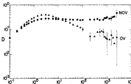
DifSusion Function

540 WOOD AND LAD0

ov

c :

O.lO- I

NOV.

l . .

“ii

t” w

0.6 . ‘r;

c . i-. 1 \

0.4 -

NOV ’

I --.,

L

1 . ’ .

. i

. “Z.

0.5 I.0

0 r? NOV --.--~

. l ?? . *-*ffift-*r--r-

-005, I I II,,,,

20 30405070100 t”

FIG. 2. The velocity autocorrelation C(t*) vs t* in the NOV and OV cases at 7 = 2.0. The plotting symbols cover the range of several realizations with N = 512, 2048, and 8192. The line is the Boltzmann approximation exp( - t*).

contradicted, so large is the scatter in Dov(t*) for t* > 100. We do note a signif- icant difference between the NOV and OV results for t* = 10 to 100, where DNoV is almost constant while Dov is definitely decreasing. And even at large values of t*,

Dov is clearly significantly smaller than DNoV . The large scatter in D(t*) for large t* is of course just the amplified “noise” from C(t*), since from (2.10) we see that

D(t*) is just the integral of C(t*). For Dov(t*) to approach zero requires that the

area under the initial positive phase of Cov(t*) be just exactly counterbalanced

by the area of the long negative tail. As the cancellation becomes nearly complete, small absolute fluctuations in Co, become large relative fluctuations in Dov . In the NOV case there is evidently little cancellation, but still the fluctuation in DNov(t*) is seen to become larger as t* increases- this is due to the accumulation of fluctuations as the t* integration is extended to very long times, as well as to a slow increase in the fluctuation in C(t*) as t* increases.

i---L

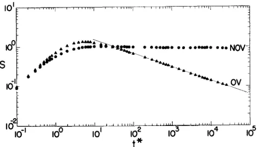
FIG. 4. The reduced mean square displacement function SW I* in the NOV and OV cases

at 7 = 2.0, as calculated for N = 8192. The estimated standard deviations are everywhere much smaller than the plotting symbols.

Reduced Mean-Square Displacement

The reduced mean-square displacement S(t*) is shown in Fig. 4. Note that the time scale here extends a decade further than in Fig. 3, and yet the fluctuations are too small to show on the scale of the figure. This is a property of the mean-square displacement function. Note that from (2.3), (2.8), (2.10), and (2.11) we have indeed

S(t*) = 4t*-’ j’* D(i*) dZ*

0

(3.1) = 2&t*)-l (u . ,:‘d2* dr(li*/u));

but we calculate S(t*) not from (3.1) but from (2.11). The equivalence of the means

of these two dynamical variables is a consequence of the time-translation invariance of the equilibrium ensemble average, but their fluctuations are different. We have also calculated the average in (3.1), as well as the similar alternative expression for D(t*),

542 WOOD AND LAD0

because comparison of the estimate (3.1) with (2.1 l), and (3.2) with (2.10) is a check upon convergence of the Monte Carlo average to the desired equilibrium ensemble average. The estimate (3.1) becomes very noisy at the largest t* values; the fluctuation may in fact be large compared to the average value, in which case the comparison is not very meaningful. But at smaller values of t* the agreement is quite good, and is additional evidence for the reliability of the Monte Carlo code and procedure. We postpone a detailed discussion of these matters to a subsequent paper.

OV Case

Returning to Fig. 4, it is seen that on this log-log plot Sov(t*) is closely approx- imated by the straight line, which has been drawn “by hand” through the data. The equation of the line is approximately

s 0” - (33/t*)0.345. _(3.3)

It is possible that a closer examination of the data may indicate that some of the small deviations from strict linearity are statistically significant; this is not a com- pletely simple question, since the fluctuations in S(t*) for two not-too-widely- separated values of t* appear to be strongly correlated (as might be expected). The OV results at still higher densities, to be reported in detail on another occasion, are similar in fitting a fractional power law over a substantial range of large t*,

with the power of t* becoming larger in magnitude as the density increases. At T = 0.5, it has been possible to follow S(t*) down to values less than 10-3, from a maximum value at small values of t* which is still of the order of unity. If (3.3) represents the correct asymptotic behavior, then it follows from (3.2) and (2.10) that C(t*) does indeed approach zero through negative values at long times.

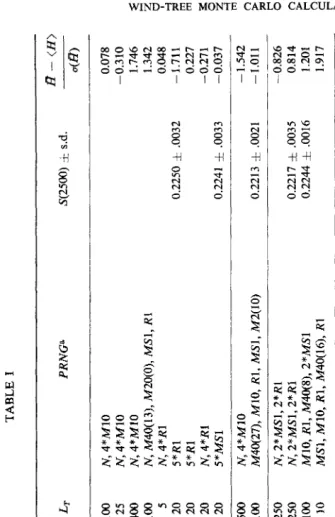
Periodicity efects. As to the possible effects of the finite period of our N = 8 192 system on these results, we note first that (3.3) and (2.33) together imply that the root-mean-square displacement (dr2)1/2 would become equal to the period only for t* M 1.5 x 105, a value considerably larger than the maximum value 25 000 of t* in Fig. 4. At t* = 25 000, (dr2)li2 = 0.55 period; slightly more than 60 % of the trajectories were observed to move more than a half-period from their initial point. On the other hand, the point t * = 2500 is well within the apparently linear region of log Sov vs log t*; at this point (dr2)lj2 m 0.26 period, and only about 5.4 % of the trajectories have moved through a half-period. Inspection of the OV entries in Table I will give some idea of the approximate lack of dependence of S(2500) on the size of the system (provided it is not too small) and on the choice of pseudo-random number generators.

TABLE I R--W> Case Real. N Lc LT PRNGa S(2500) i s.d. 40 ov

003 006 007 008 010 013 02OA 021 022 005 084 024 025 043 077

544 WOOD AND LAD0

placements are still smaller fractions of the period, lead us to believe that the OV behavior in Fig. 4 is in fact characteristic of a thermodynamically large system. The apparent validity of the extrapolation of (3.3) to infinite t” leads us to claim that, to the extent reasonably possible in calculations of this type, we have con- firmed Hauge and Cohen’s prediction that Sov(t*) + 0 as t* + co : the abnormal diffusion exists. Our apparent fractional power law (3.3) is different from the asymptotic form

so*>

t*

found by Hauge and Cohen [3, Eq. 9.41, due presumably to the effects of higher order terms in the density than those retained in the theoretical analysis.

NOV Case

The NOV results in Fig. 4 clearly show a quite different behavior. They are certainly very consistent with, but do not decisively prove, the Hauge-Cohen conclusion of normal diffusion in this case. Our reason for hedging a bit here is the very slight decrease of SNOV(t*) in Fig. 4 for t* > 100. We cannot exclude the possibility that in the NOV case, S(t*) + 0 on an even much longer time scale than that observed for the OV case. There is, of course, no known theoretical basis for such an assumption. The Hauge-Cohen theory does offer a possible explanation for the slight decay of SNov(t*), with eventual approach to a nonzero limit, in that the same diagrams which cause the “divergence” So, -+ 0 make finite contributions to SNov , and may well have a similar time-dependence.

Periodicity eflects. Some of the long-time decay in S,ov may possibly be due to periodic effects. The NOV diffusion is freer, as evidenced by the almost order-of- magnitude greater S(25 000); at t* = 25 000, (LIP)~/~ R!, 1.6 period and essentially 100 % of the trajectories have seen a half-period of the system; even at t* = 2500,

(Ar2)1/2 w 0.5 period. Again, Table I gives some quantitative comparisons of values S(2500) obtained with different values of N and with different random number generators.

Observed R vs Exact Value

We have already given in (2.28) and (2.32) the exact expression for R as a function of T and N. One can straightforwardly find the following theoretical expressions for the Monte Carlo sampling variance of R, in which (H) denotes the exact value of R:

&@) = {<H)ov[l - <H)ov1 + G - 11

@MJW,),

62 = (1 - 2y)N(l - 4y) - (1 - y)2”

+ 4y(l - 2yy f ( N ) af/(j + l)“, j=o J

y = (NT)-l, (3.6)

Ly. = Y/U - 31,

&,v(~) = W)NOV[~

- <ffhwI/&~~).

For large values of N, suitable asymptotic approximations to (3.6) are of course used for actual calculations; the quantity @ is O(N-l). For large enough values of

LC we expect the normalized deviation

u = (R - (H))/a(iT) _(3.8)

to be approximately normally distributed with zero mean and unit standard deviation for an ideally random Monte Carlo procedure. Table I gives a number of observed values of this statistic, which are seen to conform quite well to ideal behavior. These results increase our confidence in the adequacy of the pseudo- random number generators used in this investigation.

ACKNOWLEDGMENTS

This work was undertaken at the suggestion of E. G. D. Cohen, and has benefited much from his advice, as well as discussion and correspondence with E. H. Hauge. Zev Salsburg took part in the initial discussion of the problem, and in many discussions of the results as the calculations progressed. His interest and enthusiasm will be sorely missed.

We also acknowledge many helpful discussions with Jerome J. Erpenbeck. Much of the machine programming was done by Frederick R. Parker and Charles A. Slocomb.

REFERENCES

1. E. H. HAUGE AND E. G. D. COHEN, Phys. Letters 2SA (1967), 78.

546 WOOD AND LAD0

3. E. H. HAUGE AND E. G. D. COHEN, J. Math. Phys. 10 (1969), 397.

4. W. W. WOOD, Monte Carlo studies of simple liquid models in “Physics of Simple Liquids” (H. N. V. Temperley, J. S. Rowlinson and G. S. Rushbrooke, Eds.), Chap. 5, North-Holland Publishing Co., Amsterdam, 1968.

5. N. A. METROPOLIS, A. W. ROSENBLUTH, M. N. ROSENBLUTH, A. H. TELLER, AND E. TELLER, J. Chem. Phys. 21 (1953), 1087.

6. I. R. MCDONALD AND K. SINGER, Quart. Rev. 24 (1970), 238.

7. B. J. ALDER AND T. E. WAINWRIGHT, J. Chem. Phys. 31 (1959), 459. 8. A. RAHMAN, Phys. Rev. 136 (1964), A405.

9. L. VERLET, Phys. Rev. 159 (1967), 98.

10. G. D. HARP AND B. J. BERNE, Phys. Rev. A2 (1970), 975. 11. W. W. WOOD, J. Chem. Phys. 48 (1968), 415.

12. W. W. WOOD, J. Chem. Phys. 52 (1970), 729.

13. G. MARSAGLIA, Proc. Natl. Acad. Sci. U. S. 61 (1968), 25. 14. S. K. ZAREMBA, Ann. Mat. Pura. Appl. 73 (1966), 293.

15. W. A. BEYER, R. B. ROOF, AND D. WILLIAMSON,” The Lattice Structure of Multiplicative Congruential Pseudo-Random Vectors,” Los Alamos Scientific Laboratory (Los Alamos, New Mexico) preprint LA-DC-11584 (1970).