Estimation of Longitudinal Free Vibrations of
Simple Cutting Tool Models by Finite Element
Method
B.T.Sandhya1, K.Rajesh babu2, Dr.P.Venkat Ramaiah3
PG Student, Dept. of ME, S.V. University College of Engineering, Tirupathi, AP, India1 Assistant Professor, Dept. of ME, S.V. University College of Engineering.Tirupathi, AP, India2
Professor, Dept. of ME, S.V. University College of Engineering, Tirupathi, AP, India3
ABSTRACT: Any physical, structural, mechanical, fluid and heat transfer problems can well be described in a domain of interest by second order ordinary differential equations with suitable boundary conditions. The closed form or exact solutions can easily be determined for most of these problems provided if their geometries are simple in nature. However for complex geometries and arbitrary boundary conditions, finding a closed form solution is a formidable task. In such cases, approximate methods find suitable alternative to solve complex problems. In engineering applications, several approximate methods of solutions are used. One of such numerical and computer based approximate techniques is finite element method (FEM).FEM finds applications in static and dynamic analyses of mechanical structures or sub-structures. Dynamic analysis can be used to find dynamic displacements, time history and modal analysis of mechanical structures. These structures include not only machine tools but also their components and cutting tools. Dynamic analysis for simple structures can easily be carried out analytically, but for complex structures, the use of finite element method (FEM) is a must. In view of the importance attributed to the concept of FEM in engineering analysis, the present work focuses ondynamic analysis of single point cutting tool and end mill cutter by modelling them as cantilever beam and stepped shaft respectively. As a matter of fact, these tools will experience some amount of vibrations when they put to use on the corresponding machine tools. In this work, only axial or longitudinal vibrations of such tools are considered. The free vibrations of cutting tool models – cantilever beam and stepped shaft – are presented by considering simple finite line elements. In addition, the element stiffness and mass matrices of a bar or line element were utilized in determining the natural frequenciesof FE (finite element) models. The work herein highlights the dynamic analyses of cantilever beam and stepped shaft for different grid models of elastic structures. Furthermore the numerical part of this work was carried out on MATLAB and ANSYS.
KEYWORDS: Dynamic analysis, Simple cutting tools, Finite Element Method.
I. INTRODUCTION
The basic idea in the finite element method is to find the solution of a complicated problem by replacing it a simpler one. Since the actual problem is replaced by simpler one in finding the solution, we will able to find only approximate solution rather than the exact solution. The existing mathematical tools will not be sufficient to find exact solution (and sometimes, even an approximate solution) of the most practical problems. Thus, in the absence of any other convenient method to find even the approximate solution of a given problem, we have to prefer the finite element method. Moreover, the finite element method, it will often be possible to improve or refine the approximate solution by spending more computational effort.
response (like stresses and displacements) of the machine under any specified cutting (loading) condition, this structure is approximated as composed of several pieces in the finite element method. In each piece or element, a convenient approximate solution is assumed and the conditions of overall equilibrium of the structure are derived. The satisfaction of these conditions will yield an approximate solution for displacements and stresses.
1.1 Historical background
Although the name of the finite element method was given recently, the concept dates back for several centuries. For example, ancient mathematics found the circumferences of a circle by approximating it by the perimeter of a polygon In terms of the present day notation, each side of the polygon can be called a finite element. By considering the approximating polygon inscribed or circumscribed, one can obtain a lower bound or an upper bound for the true circumference. Furthermore, as the number of sides of the polygon is increased, the approximate values converge to the true value. These characteristics, as will be seen later, will hold true in any general finite element application. In recent times, an approach similar to finite element method, involving the use piecewise continuous functions defined over triangular regions, was first suggested courant in 1943 in the literature of applied mathematics. General applicability of the method.
1.2 General description of the finite element method
In the finite element method the actual continuum or body of matter, such as a solid, liquid, or gas, is represented as an assemblage of subdivisions called finite elements. These elements are considered to be interconnected at specified joints called nodes or nodal points. The nodes usually lie on element boundaries where adjacent elements are to be connected. Since the actual variation of the field variable (e.g., displacement, stress, temperature, pressure, or velocity) inside the continuum is not known, we assume that the variation of the field variable inside a finite element can be approximated by simple function. These approximating functions (also called interpolation models) are defined in terms of the values of the field variables at the nodes. When the field equations (like equilibrium equations) for the whole continuum are written, the new unknowns will be the nodal values of the field variable. By solving the field equations, which are generally in the form of matrix equations, the nodal values of field variable are known. Once these are known. Once these are known. The approximating function defines the field variable throughout the assemblage of elements.
Step (1): discretization of structure
The first step in the finite element method is to divide the structure or solution region in to sub divisions or elements. Hence the structure is to be modelled with suitable finite elements. The number, type, size, and arrangement of the elements are to be decided.
Since the displacement solution of complex structure under any specified load conditions cannot be predicted exactly, we assume some suitable solution within a element to approximate the unknown solution. The solution must be simple form a computational standpoint, but it satisfy certain convergence requirements. In general, the solution are the interpolation model is taking in the form of a polynomial.
Step (2): derivation of element stiffness matrices and load vectors
From the assumed displacement model, the stiffness matrix [Kⁱ] and the load vector pⁱ of element i are to be derived by using either equilibrium conditions or a suitable variational principle.
Step (3): assemblage of element equations to obtain the overall equilibrium equations since the structure is composed of several finite elements, the individual element stiffness matrices and load vectors are to be assembled in a suitable manner and overall equilibrium equations have to be formulated as
[k]Ф = p
Where [k] is the assembled stiffness matrix, Ф is the vector of nodal displacements, and p is the vector or nodal forces
for the complete structure.
Step (4): solution for the unknown nodal displacements
The overall equilibrium equations have to be modified to account for the boundary conditions of the problem after the incorporation of the boundary conditions, the equilibrium equation can be expressed as
[k]Ф = p
For linear problems, the vector Ф can be solved very easily. However for nonlinear problems, the solution can be
II.PROBLEM STATEMENT
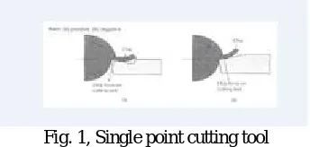
The machine tool, workpiece, and a cutting tool will form a closed loop cutting system in any manufacturing system. The accuracy and surface finish of a finished workpart would depend on the cutting dynamics of the machining system. Indeed, the cutting tool forms an important and a vital component of this closed loop system. Owing to this reason, we have identified the dynamic aspects of a cutting tool as one of the thrust areas of work to be given due consideration in manufacturing industry. Due to this fact, we have selected the following two dynamic problems of determining the longitudinal vibrations of simple cutting tool models that include single point cutting tool and an end mill cutter. The principles of vibration are equally applicable to a machine tool and its components. Consider as shown in Fig. 1, a single point tool cutting a shaft which has a keyway slot. When the tool hits the keyway slot it bounces and leaves an unwanted surface wave upon the workpiece. This is free vibration and it occurs at the resonant frequency of the tool- workpiece vibratory system.
Fig. 1, Single point cutting tool
(1) The work piece and cutting tool setup is shown in Fig. 1, wherein a cutting tool has been modelled as a cantilever beam assuming that it is fixed in a tool post. The line diagram of this cutting tool model is shown below.
Fig. 2 Single point cutting tool
Fig.3cantilever beam
The above cantilever beam model will be analyzed for its natural frequencies by discretizing it into simple finite line elements. This analysis will be carried out for different FE grid models, say 2- element, 3- element and 4- element. (2) With regard to the end milling cutter, the physical model of the same has been modelled as a stepped shaft. The physical model and the idealized model of the end mill cutter are depicted in Fig. 2 and 3 respectively. The above stepped shaft model will be analyzed for its natural frequencies by discretizing it into simple finite line elements. This analysis will be carried out for different FE grid models, say 2 – element, 3 – element and 4 – element meshes.
Fig. 5 Stepped shaft
In order to determine the natural frequencies of the above models, one should know the element stiffness matrix and element mass matrix of a line or bar elements. The following paragraphs will describe the importance and mode of deriving the above element matrices in brief.
Stiffness Matrix
The primary characteristics of a finite element are embodied in the element stiffness matrix. For a structural finite element, the stiffness matrix contains the geometric and material behavior information that indicates the resistance of the element to deformation when subjected to loading. Such deformation may include axial, bending, shear, and torsional effects. For finite elements used in nonstructural analyses, such as fluid flow and heat transfer, the term stiffness matrix is also used, since the matrix represents the resistance of the element to change when subjected to external influences.
k =∫ EAφi(x)φj(x)dx (1)
By making use of shape functions and performing the integration of the above integral, we obtain the following element stiffness matrix for a line element;
Element stiffness matrix, k = 1 −1
−1 1 (2)
Similarly, the mass matrix can also be derived as follows:
The mass matrix is built up from element contributions, and we start at that level construction of the mass matrix of individual elements with distributed mass density.
m =∫ λ ∅(x)∅(x)dx(3)
Element mass matrixm = 2 1
1 2(4)
The above matrices are going to be used in the dynamic analysis of the cutting tools models. The detailed FE analyses (both on MATLAB platform and ANSYS platform) of the above beams are given in the subsequent Chapters. Besides, analytic solutions (exact solution) of the above models are also highlighted in this work.
III.MATHEMATICAL FORMULATION
Differential equation for 1D element:
EA + . = (5)
E + . = (6)
+ . =0(7)
= (8)
Kinematic assumptions within a element
U(x,t)= (x) (t)+ (x) (t)
(x)=1-x/L
+ . = 0
+ . =0
∫ + ∫ = 0(9)
K M Integrating the above equation we get the stiffness matrix
=∫ ( ) ( )dx
=∫ ö ( ) ( )dx
=∫ (1− )(1− )dx
=∫ (1− ) dx
=
=∫ ( ) ( )dx
=∫ (1− )( )dx
= -
=
=∫ ( )ö ( )dx
=∫ ( )( )dx
=
Stiffness matrixK = , = 1 −1
−1 1 (10)
Mass matrix;
=∫ ( ) ( )dx
=∫ ( ) ( )dx
=∫ (1− )(1− )dx
=
=∫ ( ) ( )dx
=∫ (1− )( )dx
=
=∫ ( ) ( )dx
=∫ ( )( )dx
=
Mass matrix M= , M = 2 1
1 2 (11)
INVERSE FUNCTION =K- = 0
1 −1
−1 1 −
2 1 1 2 =0
IV. RESULTS AND DISCUSSION
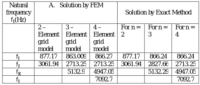
As stated in problem definition, simple cutting tools (turning tool and an end mill cutter) have been modeled as a cantilever beam and stepped shaft respectively. The mathematical idealization of real cutters has been done through finite element modeling. Any cutting tool when pressed in to operation will undergo slight vibrations depending upon the selected cutting conditions. Owing to this fact, the above cutting tool models have been analyzed from the viewpoint of their longitudinal (axial) vibrations. As such the cutting tool models would experience vibrations in all three Cartesian coordinates-x, y, and z. However, the work herein has focused on axial vibrations of selected models. It is to be noted that the real dimensions of the cutting tools were not considered in the present analysis. However, the procedural aspects as detailed in this dissertation can easily be extended to real numerical values without any difficulty. So far as cantilever beam model is concerned. The axial vibrations of the same have been determined by discretizing it into 2 – element, 3 – element and 4 – element grid models. This sort of analysis has been carried out by considering two different sets of geometric parameters and material properties of beams. In addition, the exact solution of the cantilever beam model has also been given from the fundamental mathematical differential equations. Besides solving the beam model by a GUI based ANSYS tool. The following tables and ANSYS platform plates highlight the results as obtained by FEM, ANSYS and Exact method.
Table 1 and 2 Comparison of solutions of cantilever beam by FEM, ANSYS, and Exact method
Natural frequency
f(Hz)
A. Solution by FEM
Solution by Exact Method 2 –
Element grid model
3 – Element grid model
4 – Element grid model
For n = 2
For n = 3
For n = 4
f 877.17 863.009 866.27 877.17 866.24 866.24
f 3061.94 2713.25 2713.25 3061.94 2827.66 2713.25
f 5132.9 4947.05 5132.29 4947.05
Fig 6 Second natural frequency of two element grid model as depicted by ANSYS package
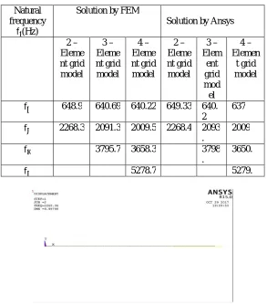
Fig.7 First natural frequency of two element grid model as depicted by ANSYS package Natural
frequency
f(Hz)
Solution by FEM
Solution by Ansys 2 –
Eleme nt grid model
3 – Eleme nt grid model
4 – Eleme nt grid model
2 – Eleme nt grid model
3 – Elem
ent grid mod el
4 – Elemen
t grid model
f 648.9 640.69 640.22 649.33 640. 2
637
f 2268.3 2091.3 2009.5 2268.4 2093 .
2009
f 3795.7 3658.3 3798
.
3650.
Fig. 8 First natural frequency of three element grid model as depicted by ANSYS package
From the above tables, and plots, it is clear that as the number of elements increases, the approximate solution by FEM was approaching to the Exact Solution. However, as the mass of beam decreases, the natural frequency of the beam increases. Coming to a stepped shaft model of an end mill cutter, the procedure as described for a cantilever beam model was followed in principle. The corresponding natural frequencies and the associated ANSYS plates were listed in the tables 1 and figures 2, 3.
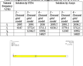
Table 3 Comparison of solutions of stepped shaft by FEM, ANSYS.
Fig 9 First natural frequency of two element grid model as depicted by ANSYS package Natural
frequency (Hz)
Solution by FEM Solution by Ansys
2 – Element grid model
3 – Element grid model
4 – Element grid model
2 – Element grid model
3 – Element grid model
4 – Element grid model 2095 2091 2036 2095.5 2091.2 2036.2 6147 5772.6 5711.1 6150.3 5779.1 5712.0
12342.5 10950 12345 10952
Fig 10 First natural frequency of three element grid model as depicted by ANSYS package
From the above tables and figures, it is evident that the knowledge of natural frequencies of above cutting tools would aid the operator to select the cutting conditions such that tools shall be allowed to run well below the fundamental natural frequencies as listed in the respective tables. Ultimately, the work herein gives firsthand information about the natural frequencies of simple cutting tool models.
VI.CONCLUSIONS
In this work an attempt has been made to determine the longitudinal vibrations of simple cutting tool models by finite element method. The selected cutting tools have been modeled as simple cantilever beam and a stepped shaft beam. The vibration analysis has been carried out by discretizing the cutting tool models into finite bar elements. The associated stiffness and mass matrices were utilized in arriving at desired circular natural frequencies and the corresponding eigenvectors and mode shapes of the cantilever beam and stepped shaft models. The pattern of mode shape plots were in agreement with those of the established patterns of the cantilever beams as in solid mechanics. It is further noted that as the mass of the member decreases, the natural frequencies of the beam would increase. The present work also throws some light on the utility of the exact methods in solving the given beam models besides solving the problem by ANSYS. It is anticipated that the frequency values as reported in the present work would aid the designer in selecting the suitable cutting conditions while machining a workpart. To say explicitly, the cutting tools (turning tool and end mill cutter) have to be operated well below the circular frequency values as highlighted in this work. Allowing the tools/cutters to run below the stated natural frequencies would results in good surface finish of the finished component.
REFERENCES
1. Tirupathi R. Chandrupatla, Ashok D. Belegundu, “Introduction to Finite Elements in Engineering, august, 2002 2. C S Krishnamurthy, “ FEA (Finite Element Analysis)”
3. Central institute of tool design course material “ANSYS”
4. Singiresu S.Rao, “Introduction To The Finite Element Method (FEM)” 5. Bathe, “ Finite Element Procedures”