ABSTRACT
MATTHEWS, JESSICA LOOCK. Sensitivity Analysis and Development of a Model that Quantifies the Effect of Soil Moisture and Plant Age on Leaf Conductance. (Under the direction of Ralph Smith.)
Global climate models are complex compilations of a number of inter-related submodels. Typical implementations include modules for atmospheric, oceanic, sea ice, and land interac-tions. Our focus is on the photosynthesis submodel of these larger global climate models, which is lacking either by it’s omittance or it’s oversimplification in many climate models.
A recent model by Niyogi et al. [48] links environmental conditions and plant physiological processes to closely coupled photosynthesis and leaf conductance rates. We start by carefully describing this model and performing sensitivity analysis to characterize the response of model state variables, namely photosynthetic rate, to changes in model parameter values. A novel data set produced from a unique water stress field studying four different levels of watering conditions with two different genotypes of soybeans over the course of two growing seasons is employed for model validation. This data set is applied to the model of Niyogi et al. to test model accuracy under varying soil moisture conditions. It is our conclusion that this model requires refinement to accurately predict total leaf conductance.
Sensitivity Analysis and Development of a Model that Quantifies the Effect of Soil Moisture and Plant Age on Leaf Conductance
by
Jessica Loock Matthews
A dissertation submitted to the Graduate Faculty of North Carolina State University
in partial fulfillment of the requirements for the Degree of
Doctor of Philosophy
Applied Mathematics
Raleigh, North Carolina
2010
APPROVED BY:
H. T. Banks Edwin Fiscus
Mansoor Haider Ralph Smith
DEDICATION
BIOGRAPHY
The author was born in Carroll County, Maryland. After graduation from North Carroll High School in Hampstead, Maryland she attended two Pennsylvania colleges including Pennsylva-nia State University and York College where she explored such subjects as architecture and photography. As the confusion of teenage angst waned, she wandered to Raleigh, North Car-olina due to the generosity of her older brother offering his hospitality. Here she gained focus and rediscovered her passion for studying mathematics. While in Raleigh she met a wonderful native southerner, Quint Kindley, whom she married in 2008.
ACKNOWLEDGEMENTS
Firstly, I would like to thank my advisor Dr. Ralph Smith for his direction, patience, and kindness throughout the years. Thanks also to my committee including Dr. H.T. Banks, Dr. Edwin Fiscus, and Dr. Mansoor Haider whom have all been a pleasure to work with during this entire process. I am especially grateful to Dr. Fiscus for generously providing the data that appears in this dissertation.
I want to thank all my colleagues at SRA International, Inc. who encouraged me to pursue my Ph.D. and were supportive throughout the process. Most especially I’d like to thank Marjo, Mike, Pat, Nicole, and Shawn. I will miss you all!
TABLE OF CONTENTS
List of Tables . . . vii
List of Figures . . . .viii
Chapter 1 Introduction . . . 1
Chapter 2 Analysis of Existing Work . . . 4
2.1 Background . . . 4
2.1.1 C3 Species . . . 5
2.1.2 C4 Species . . . 13
2.2 Model Solution . . . 14
2.2.1 C3 Species . . . 17
2.2.2 C4 Species . . . 19
2.2.3 Root Finding . . . 20
2.3 Sensitivity Analysis . . . 23
2.3.1 Surface Temperature Ts . . . 23
2.3.2 Canopy Temperature Tc . . . 23
2.3.3 Ambient Temperature Ta . . . 25
2.3.4 Surface PressureP . . . 25
2.3.5 Wind Speed u . . . 26
2.3.6 Oxygen Availability in Leaf Cells O2 . . . 27
2.3.7 Photosynthetically Active Radiation P AR . . . 27
2.3.8 Relative Humidity at Leaf Surface hs. . . 28
2.3.9 Ambient CO2 Partial PressureCa . . . 30
2.3.10 Root Level Soil Moisture Wilting Value wwilt, Field Capacity Valuewf c, and Deep Soil Moisture Content w2 . . . 30
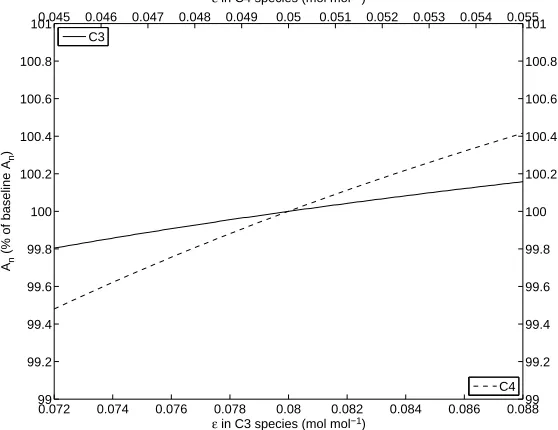
2.3.11 Quantum Efficiency for Carbon Dioxide Uptake . . . 33
2.3.12 Leaf-Scattering Coefficient for P AR wπ . . . 33
2.3.13 Factor to Account for Different Diffusivities of H2O and CO2 in the Stom-atal Pores η . . . 34
2.3.14 Vegetation Stress Factors, S2 (high) and S4 (low) . . . 35
2.3.15 Maximum Catalytic Rubisco Capacity for Leaf Vmax . . . 36
2.3.16 Maximum Net Assimilation RateAm,max . . . 37
2.3.17 Potential Maximum Value of Mesophyllic Conductancegmp . . . 39
2.3.18 Transfer Coefficient c. . . 40
2.3.19 Leaf Length Scale, d . . . 41
2.3.20 Coupling Coefficients,β1 and β2 . . . 42
2.3.21 Slope mand Intercept b in Stomatal Conductance Equation . . . 44
2.3.22 Coefficient of ws Equation . . . 46
2.3.25 Constants in S Equation . . . 50
2.3.26 Constants in Kc and Ko Equations . . . 50
2.3.27 Constants in gbf c and gbf r Equations . . . 52
2.3.28 Comparison of Parameter Sensitivity . . . 52
Chapter 3 Data Analysis and Niyogi Model Performance . . . 54
3.1 Data . . . 54
3.1.1 Description of Experimental Procedure . . . 54
3.1.2 Soil Moisture Data . . . 55
3.1.3 Barometric Pressure . . . 62
3.1.4 Ambient CO2 Levels . . . 63
3.1.5 Relative Humidity . . . 65
3.1.6 Photosynthetically Active Radiation (PAR) . . . 65
3.1.7 Temperature . . . 67
3.1.8 Wind . . . 69
3.1.9 Leaf Conductance . . . 71
3.2 Niyogi Model Performance . . . 77
Chapter 4 Model Development and Calibration. . . 84
4.1 Model Development . . . 84
4.2 Model Calibration . . . 85
4.3 Confidence Intervals for Parameter Estimates . . . 93
4.3.1 Asymptotic Theory . . . 93
4.3.2 Bootstrap Method . . . 95
4.4 Confidence Intervals for Model Predictions . . . 103
4.4.1 Asymptotic Theory . . . 104
4.4.2 Monte Carlo Method . . . 108
4.4.3 Bootstrap Method . . . 112
4.5 Comparison of Proposed Model to Niyogi’s Model . . . 115
Chapter 5 Conclusions and Future Work . . . .116
LIST OF TABLES
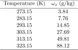
Table 2.1 Saturation mixing ratio (ωs) values at varying temperatures andP = 1000
millibars. . . 9
Table 2.2 Model parameters from Niyogi et al. [48]. . . 15
Table 2.3 Soil moisture parameter values from Jacquemin and Noilhan [34]. Note that wf c values are associated with a hydric conductivity of 0.1 mm/day and wwilt values correspond to a moisture potential of -15 bar. . . 32
Table 2.4 Comparison of An values for different uses of cfor C3 plants. . . 41
Table 2.5 Comparison of values (µmol m−2 s−1) for limiting factors and resultant assimilation rates. . . 43
Table 3.1 Significant growing season events. . . 55
Table 3.2 Conductance data point summary. . . 78
Table 3.3 Soil parameter values derived from data. . . 78
Table 3.4 Species-specific model parameter values used for simulation. . . 79
Table 3.5 Sum of squared errors. . . 82
Table 3.6 Normalized sum of squared errors. Each entry is the SSE value divided by 105. The values in parenthesis are the number of data points used for that experiment. . . 83
Table 4.1 Parameter space regions utilized with initial global search. . . 85
Table 4.2 Parameter estimates for each case. . . 87
Table 4.3 95% confidence intervals derived from the wild bootstrap method using the percentile method for each case. . . 102
Table 4.4 95% confidence intervals derived from (4.11) and (4.30) applying wild bootstrap simulations to estimate covariance matrices for each case. . . 103
Table 4.5 Percentage of data points covered by estimated 95% confidence regions computed using (4.32). . . 106
Table 4.6 Percentage of data points covered by estimated 95% confidence regions computed with Monte Carlo methods. . . 109
Table 4.7 Percentage of data points covered by estimated 95% confidence regions computed with percentile methods and bootstrap simulations. . . 112
LIST OF FIGURES
Figure 2.1 Schematic transverse section of an (a) C3 and (b) C4 leaf. . . 5
Figure 2.2 Response ofAnto surface temperature Ts. . . 24
Figure 2.3 Response ofAnto canopy temperatureTc. . . 24
Figure 2.4 Response ofAnto ambient temperatureTa. . . 25
Figure 2.5 Response ofAnto surface pressure P. . . 26
Figure 2.6 Response ofAnto wind speed u. . . 27
Figure 2.7 Response ofAnto oxygen availability in leaf cells O2. . . 28
Figure 2.8 Response ofAnto photosynthetically active radiation P AR. . . 29
Figure 2.9 Response ofAnto relative humidity at leaf surface hs. . . 29
Figure 2.10 Response of Anto ambient CO2 partial pressureCa. . . 31
Figure 2.11 Response of Anto f(w2). . . 32
Figure 2.12 Response of Anto quantum efficiency for carbon dioxide uptake . . . 33
Figure 2.13 Response of Anto leaf-scattering coefficient for P AR wπ. . . 34
Figure 2.14 Response of Anto the factor to account for different diffusivities of H2O and CO2 in the stomatal pores, η. . . 35
Figure 2.15 Response of Anto vegetation stress factors (a) S2 and (b)S4. . . 36
Figure 2.16 Response of Anto maximum catalytic Rubisco capacity for leaf Vmax. . . 37
Figure 2.17 Response of Anto maximum net assimilation rate Am,max. . . 38
Figure 2.18 Response of Anto a different Am,max formulation based on temperature. 39 Figure 2.19 Response ofAnto potential maximum value of mesophyllic conductance gmp. . . 40
Figure 2.20 Response of Anto transfer coefficient c. . . 41
Figure 2.21 Response of Anto leaf length scale d. . . 42
Figure 2.22 Response of Anto coupling coefficients (a) β1 and (b)β2. . . 43
Figure 2.23 Response of Anto coupled changes in β1 and β2 in C3 species. . . 44
Figure 2.24 Response of Anto coupled changes in β1 and β2 in C4 species. . . 44
Figure 2.25 Response of An to (a) slope m and (b) intercept b in stomatal conduc-tance equation. . . 45
Figure 2.26 Response of Anto m and b in C3 species. . . 46
Figure 2.27 Response of Anto m and b in C4 species. . . 46
Figure 2.28 Response of Anto coefficient ofws equation. . . 47
Figure 2.29 Response of Anto coefficient ofRd equation. . . 48
Figure 2.30 Response of An to coefficient in (a) numerator and (b) denominator of gm equation. . . 49
Figure 2.31 Response of An to coefficient in (a) numerator and (b) denominator of f(T) equation. . . 49
Figure 2.36 Maximum percent change in An over parameter ranges defined in
previ-ous subsections for C3 plants. . . 53
Figure 2.37 Maximum percent change in An over parameter ranges defined in previ-ous subsections for C4 plants. . . 53
Figure 3.1 Field diagram for 2008 growing season. Color coding of experiments is as follows: Green (open), Red (wet), Yellow (medium), Brown (dry), Gray (border, unsampled). Horizontal hashed areas represent Haskell plant areas and open sections represent N01 areas. The white circles represent approximate locations of tubes where soil moisture measurements were collected. . . 56
Figure 3.2 Field diagram for 2009 growing season. Color coding of experiments is as follows: Green (open), Red (wet), Yellow (medium), Brown (dry), Gray (border, unsampled). Horizontal hashed areas represent Haskell plant areas and open sections represent N01 areas. The white circles represent approximate locations of tubes where soil moisture measurements were collected. . . 56
Figure 3.3 Soil moisture content for the “dry” experimental plot in 2008. . . 57
Figure 3.4 Soil moisture content for the “medium” experimental plot in 2008. . . 58
Figure 3.5 Soil moisture content for the “wet” experimental plot in 2008. . . 58
Figure 3.6 Soil moisture content for the “open” experimental plot in 2008. . . 59
Figure 3.7 Soil moisture content averages for all experimental plots in 2008. . . 59
Figure 3.8 Soil moisture content for the “dry” experimental plot in 2009. . . 60
Figure 3.9 Soil moisture content for the “medium” experimental plot in 2009. . . 60
Figure 3.10 Soil moisture content for the “wet” experimental plot in 2009. . . 61
Figure 3.11 Soil moisture content for the “open” experimental plot in 2009. . . 61
Figure 3.12 Soil moisture content averages for all experimental plots in 2009. . . 62
Figure 3.13 Barometric pressure data from 2008 and 2009 growing seasons. . . 63
Figure 3.14 Minimum, mean, and maximum ambient carbon dioxide levels during the 2008 growing season. . . 64
Figure 3.15 Minimum, mean, and maximum ambient carbon dioxide levels during the 2009 growing season. . . 64
Figure 3.16 Relative humidity data. Stars are relative humidity values from the 2008 growing season and circles are data from 2009. . . 66
Figure 3.17 PAR data from 2008 growing season. . . 66
Figure 3.18 PAR data from 2009 growing season. . . 67
Figure 3.19 Cuvette temperature versus leaf temperature. Stars are values from the 2008 growing season, and circles are data from 2009. . . 68
Figure 3.20 Weather station temperature readings during the 2008 and 2009 growing seasons. . . 68
Figure 3.21 Wind speed data from 2008 growing season. . . 70
Figure 3.23 Conductance data from “dry” experimental plot in 2008. Red circles and lines indicate Haskell genotype, Green stars and lines indicate N01 genotype. Stars/circles are individual data points while lines represent means. . . 71 Figure 3.24 Conductance data from “medium” experimental plot in 2008. Red circles
and lines indicate Haskell genotype, Green stars and lines indicate N01 genotype. Stars/circles are individual data points while lines represent means. . . 72 Figure 3.25 Conductance data from “wet” experimental plot in 2008. Red circles
and lines indicate Haskell genotype, Green stars and lines indicate N01 genotype. Stars/circles are individual data points while lines represent means. . . 72 Figure 3.26 Conductance data from “open” experimental plot in 2008. Red circles
and lines indicate Haskell genotype, Green stars and lines indicate N01 genotype. Stars/circles are individual data points while lines represent means. . . 73 Figure 3.27 Conductance data averages for all experimental plots with Haskell
geno-type in 2008. . . 73 Figure 3.28 Conductance data averages for all experimental plots with N01 genotype
in 2008. . . 74 Figure 3.29 Conductance data from “dry” experimental plot in 2009. Red circles
and lines indicate Haskell genotype, Green stars and lines indicate N01 genotype. Stars/circles are individual data points while lines represent means. . . 74 Figure 3.30 Conductance data from “medium” experimental plot in 2009. Red circles
and lines indicate Haskell genotype, Green stars and lines indicate N01 genotype. Stars/circles are individual data points while lines represent means. . . 75 Figure 3.31 Conductance data from “wet” experimental plot in 2009. Red circles
and lines indicate Haskell genotype, Green stars and lines indicate N01 genotype. Stars/circles are individual data points while lines represent means. . . 75 Figure 3.32 Conductance data from “open” experimental plot in 2009. Red circles
and lines indicate Haskell genotype, Green stars and lines indicate N01 genotype. Stars/circles are individual data points while lines represent means. . . 76 Figure 3.33 Conductance data averages for all experimental plots with Haskell
geno-type in 2009. . . 76 Figure 3.34 Conductance data averages for all experimental plots with N01 genotype
in 2009. . . 77 Figure 3.35 Conductance predictions g` versus data for all experimental plots with
Haskell genotype in 2008. The 45◦ line is superimposed to indicate the
Figure 3.36 Conductance predictions g` versus data for all experimental plots with N01 genotype in 2008. The 45◦ line is superimposed to indicate the scale
of underprediction. . . 80 Figure 3.37 Conductance predictions g` versus data for all experimental plots with
Haskell genotype in 2009. The 45◦ line is superimposed to indicate the
scale of underprediction. . . 81 Figure 3.38 Conductance predictions g` versus data for all experimental plots with
N01 genotype in 2009. The 45◦ line is superimposed to indicate the scale
of underprediction. . . 81
Figure 4.1 Conductance predictions versus data for all experimental plots with the Haskell genotype in 2008. The 45◦ line is superimposed to indicate scale. 88
Figure 4.2 Conductance predictions (dotted lines) compared to mean data by date (solid lines) for the Haskell genotype in 2008. . . 88 Figure 4.3 Conductance predictions versus data for all experimental plots with the
N01 genotype in 2008. The 45◦ line is superimposed to indicate scale. . . 89
Figure 4.4 Conductance predictions (dotted lines) compared to mean data by date (solid lines) for the N01 genotype in 2008. . . 89 Figure 4.5 Conductance predictions versus data for all experimental plots with the
Haskell genotype in 2009. The 45◦ line is superimposed to indicate scale. 90
Figure 4.6 Conductance predictions (dotted lines) compared to mean data by date (solid lines) for the Haskell genotype in 2009. . . 90 Figure 4.7 Conductance predictions versus data for all experimental plots with the
N01 genotype in 2009. The 45◦ line is superimposed to indicate scale. . . 91
Figure 4.8 Conductance predictions (dotted lines) compared to mean data by date (solid lines) for the N01 genotype in 2009. . . 91 Figure 4.9 Model plant age dependence curves f(t;θ) as described by (4.2) and
Table 4.2. . . 92 Figure 4.10 Model soil moisture dependence curvesh(w2;θ) as described by (4.3) and
Table 4.2. . . 92 Figure 4.11 Conductance predictions versus residuals. (a) Haskell genotype in 2008,
(b) N01 genotype in 2008, (c) Haskell genotype in 2009, and (d) N01 genotype in 2009. . . 97 Figure 4.12 Histograms of bootstrapped parameter estimates ofα0−α3 and β1−β3
for the Haskell genotype in 2008. . . 99 Figure 4.13 Histograms of bootstrapped parameter estimates ofα0−α3 and β1−β3
for the N01 genotype in 2008. . . 100 Figure 4.14 Histograms of bootstrapped parameter estimates ofα0−α3 and β1−β3
for the Haskell genotype in 2009. . . 100 Figure 4.15 Histograms of bootstrapped parameter estimates ofα0−α3 and β1−β3
for the N01 genotype in 2009. . . 101 Figure 4.16 95% confidence regions computed with (4.32) (dotted lines) compared to
Figure 4.17 95% confidence regions computed with (4.32) (dotted lines) compared to mean data by date (solid lines) for the N01 genotype in 2008. . . 107 Figure 4.18 95% confidence regions computed with (4.32) (dotted lines) compared to
mean data by date (solid lines) for the Haskell genotype in 2009. . . 107 Figure 4.19 95% confidence regions computed with (4.32) (dotted lines) compared to
mean data by date (solid lines) for the N01 genotype in 2009. . . 108 Figure 4.20 95% confidence regions computed with Monte Carlo methods (dotted
lines) compared to mean data by date (solid lines) for the Haskell genotype in 2008. . . 110 Figure 4.21 95% confidence regions computed with Monte Carlo methods (dotted
lines) compared to mean data by date (solid lines) for the N01 genotype in 2008. . . 110 Figure 4.22 95% confidence regions computed with Monte Carlo methods (dotted
lines) compared to mean data by date (solid lines) for the Haskell genotype in 2009. . . 111 Figure 4.23 95% confidence regions computed with Monte Carlo methods (dotted
lines) compared to mean data by date (solid lines) for the N01 genotype in 2009. . . 111 Figure 4.24 95% confidence regions computed with percentile methods and bootstrap
simulations (dotted lines) compared to mean data by date (solid lines) for the Haskell genotype in 2008. . . 113 Figure 4.25 95% confidence regions computed with percentile methods and bootstrap
simulations (dotted lines) compared to mean data by date (solid lines) for the N01 genotype in 2008. . . 113 Figure 4.26 95% confidence regions computed with percentile methods and bootstrap
simulations (dotted lines) compared to mean data by date (solid lines) for the Haskell genotype in 2009. . . 114 Figure 4.27 95% confidence regions computed with percentile methods and bootstrap
Chapter 1
Introduction
Climate change is a current topic of great controversy in today’s world. The arguments formed by every side stem from the problem that no one can predict the future. Although we can not tell with absolute certainty what the future holds for the earth, we do have the technology to produce mathematical models to predict outcomes and their associated prediction variabilities. Global climate models are complex compilations of a number of inter-related submodels. Typical implementations include modules for atmospheric, oceanic, sea ice, and land interac-tions. Currently, a number of models exist but, since every model is a simplification of reality, improvements can always be made. Our focus is on the photosynthesis submodel of these larger global climate models. This component is lacking either by it’s omittance or it’s oversimplifi-cation in many climate models. In particular, we examine two models from the bank of models used by the Intergovernmental Panel on Climate Change (IPCC) to generate climate change predictions [55]. The model created by the National Oceanic and Atmospheric Administration (NOAA) omits entirely any photosynthesis component and the inclusion of stomatal conduc-tance does not account for water-stressed conditions [45]. The model created by the National Center for Atmospheric Research (NCAR) includes a photosynthesis submodel based on the formulation presented by Collatz et al. [21], however there is no mechanism for change in stomatal conductance due to moisture conditions [53].
the model will return lower than actual predictions of ambient carbon dioxide. Conversely, if photosynthetic capacity is underestimated, the carbon dioxide levels will be overpredicted. Potential impacts of climate change include periods of drought as well as the greater possibility of extreme precipitation events [44]. Because of the importance of correctly characterizing pho-tosynthetic processes in the context of climate modeling, it is imperative that the response of photosynthesis to drought and extreme precipitation events be well understood and correctly modeled.
A number of models describing photosynthesis have been created over the years. Many [2, 21, 47, 60] are based on the so-called Ball-Berry model
gs=m
Anhs
Cs
+b, (1.1)
where gs represents stomatal conductance (mol air m−2 s−1), An represents the net photo-synthesis rate (µmol CO2 m−2 s−1), hs is the decimal relative humidity at the leaf surface (unitless),Cs is the CO2 concentration at the leaf surface (µmol mol−1 air), andmand b(mol
m−2 s−1) are the species-specific slope and intercept terms, respectively.
The model presented in Niyogi et al. [48] uses (1.1) as a basis for linking plant physiological and ecological processes to stomatal conductance calculations. The model characterizes a num-ber of biological mechanisms through the incorporation of dependencies on oxygen availability, temperature, species-specific maximum assimilation rate, soil moisture, wind, ambient pres-sure, leaf length, photosynthetically active radiation (PAR), and leaf scattering of PAR. Given the inclusion of these many mechanisms and model validation under idealized environmental conditions [48], we chose this model as a candidate for extension to accurately predict stomatal conductance and photosynthesis rates under water-stressed conditions in soybeans.
Chapter 2
Analysis of Existing Work
2.1
Background
The world of plants can be divided into three categories according to their photosynthetic processes: C3, C4, and CAM.
The vast majority of plants perform C3 photosynthesis, which is named C3 because atmo-spheric carbon dioxide (CO2) is first incorporated into a three-carbon molecule in this
photo-synthetic process. This carbon fixation is catalyzed by the Rubisco enzyme. Rubisco has dual carboxylase and oxygenase activity, meaning that atmospheric oxygen (O2) instead of CO2may
be consumed during the alternative process of photorespiration. This results in less photosyn-thesis because the Rubsico enzyme is being utilized during the opposite reaction. However, C3 photosynthesis is more efficient than C4 and CAM under cool, moist, and normal light conditions because fewer enzymes are involved in the process. Common examples of C3 species include soybeans, rice, and cotton.
C4 plants are considered to be more advanced than their C3 counterparts. Bypassing the photorespiration pathway, C4 plants convert atmospheric CO2to a four-carbon compound in the
mesophyll cells catalyzed by the phosphoenolpyruvate carboxylase (PEP-carboxylase) enzyme. This compound is then shuttled to the bundle sheath cells where CO2 is delivered to continue
processing along the conventional C3 pathway. This alternative delivery method enables C4 plants to photosynthesize faster than C3 plants in high light and high temperature conditions while avoiding photorespiratory losses. Figure 2.1 illustrates the anatomical differences between C3 and C4 plants [49]. C4 plants also exhibit better water use efficiency because their stomata do not need to remain open as long since their photosynthetic process is more efficient [10]. Corn, sugarcane, and crabgrass are a few of the thousands of identified C4 species.
(a) (b)
Figure 2.1: Schematic transverse section of an (a) C3 and (b) C4 leaf.
succulents and differ from C3 and C4 plants because their stomata open at night rather than during the day. Atmospheric CO2entering the leaf is converted to an acid and stored overnight
until breaking down and releasing the CO2 to Rubisco for photosynthesis during the day when
abundant light energy is available. These plants thrive in arid conditions because their stomata open at night thus avoiding transpirational losses due to radiative heating. The small fraction of the plant kingdom which utilizes CAM photosynthesis includes many orchids, pineapple, and all varieties of cactus.
With the modification of a few equations and parameters the model in [48], analyzed sub-sequently, is applicable to both C3 and C4 plant species.
2.1.1 C3 Species
In plants, stomata are pores on the leaf and stem used for gas exchange. Oxygen produced by photosynthesis exits through the stomata which also restricts the outward flux of water (transpiration). Inward diffusion of air containing CO2 and O2 to sustain photosynthesis and
respiration, respectively, also occurs through the stomata. Environmental variables affecting stomatal aperture include temperature, air humidity, wind speed, light intensity, water stress, and CO2 concentration.
The model presented in Niyogi et al. [48] employs a stomatal model linking plant physio-logical and ecophysio-logical processes to stomatal conductance calculations. In particular, they use the relative-humidity-based approach, introduced by Ball et al. [4] and expanded in Ball [5], which yields the relation
gs=m
AnhsP
Cs
Here gs represents stomatal conductance (mol air m−2 s−1), An represents the net photosyn-thesis rate (mol CO2m−2s−1),hsis the decimal relative humidity at the leaf surface (unitless), P is the surface pressure (Pa), Cs is the CO2 partial pressure at the leaf surface (Pa), and m
(unitless) andb (mol m−2 s−1) are the species-specific slope and intercept terms, respectively.
Note that we have included the surface pressureP, which was omitted from [48] but is required for unit balance. This so-called Ball-Berry model given in (2.1) is frequently a basis for coupled leaf photosynthesis and stomatal conductance models [2, 3, 21, 22, 47, 60]. The robustness of this model was validated in [5] with more than 500 data points from plants of 13 different species grown under varying light and nutrient conditions. It is noted that values for m and b are species specific, wherem tends to be smaller in the C4 species than C3. Also, as An tends towards zero, as a result of low photon flux or low ambient CO2 concentrations, the stomatal
response is no longer linear meaning this model is not a good approximation of the kinetics. Therefore when applying this model, one must take notice of these environmental conditions [5].
Remark. To adhere to proper units in the calculation of gs, the surface pressure term P is necessary. Although this term was omitted by [48], this corrected formulation is required when Cs is defined as partial pressure rather than concentration.
The net photosynthesis rate is defined as
An=Ag−Rd (2.2)
where Ag is the gross carbon assimilation rate (mol CO2 m−2 s−1) and Rd is the rate of CO2
evolution resulting from processes other than photorespiration which is known as the dark respiration rate (mol CO2 m−2 s−1). This equation seems to gain recognition with the work of
Farquhar et al. [29] and is recurrent in the modeling literature [3, 21, 22, 47, 60, 63, 66].
Gross Carbon Assimilation Rate
The gross carbon assimilation rate is determined by three limiting factors
• Rubisco (wc)
• Light (we)
• Plant capacity to utilize photosynthesis products (ws)
β1w2p−wp(wc+we) +wewc = 0 (2.3)
β2A2g−Ag(wp+ws) +wpws= 0 (2.4)
wherewp is an interim variable representing the rate limitation imposed by Rubisco and light, and theβ’s are coupling coefficients.
Rubisco limitation: Rubisco, the common name for Ribulose-1,5-bisphosphate carboxylase oxygenase, is an enzyme used in the first step of the Calvin cycle, which is a series of biochemical reactions that take place in photosynthetic organisms to convert CO2 into organic compounds
for use by the organism. Following Collatz et al. [21], the first limitation to the C3 gross photosynthesis rate is quantified by the relation
wc=Vm
Ci−Γ∗
Ci+Kc(1 +KO2o)
(2.5)
where Vm represents the catalytic Rubisco capacity for the leaf (mol CO2 m−2 s−1), Ci is the partial pressure of CO2 in intercellular spaces (Pa), Γ∗ is the compensation point (Pa), Kc is the Michaelis-Menten constant for CO2 (Pa), O2 is the oxygen availability in leaf cells (Pa),
and Ko is the oxygen inhibition constant (Pa). Similar formulations for the Rubisco limitation on photosynthesis in C3 plants are found in [29, 47, 60, 63].
Niyogi et al. [48] developed the unique representation
Vm =Vmaxf(T)f(w2)2.1Q10 (2.6)
which includes dependencies on both temperature and soil moisture. Vmaxdefines the maximum Rubisco catalytic capacity (mol CO2 m−2 s−1),f(T) is the temperature-dependence (unitless),
andf(w2) is the soil moisture dependence (unitless). The unitless temperature-dependent term
Q10 is defined as
Q10=
Ts−298.0
10 (2.7)
f(T) = 2
Q101 +e0.3(S4−Ts)
1 +e0.3(Ts−S2) (2.8)
where S2 and S4 are the high and low vegetation stress factors, respectively. The motivation
for including this formulation of temperature dependency is to approximate the response of C4 plants to extreme temperatures [9]. A similar equation is utilized in Sellers et al. [60], with the exception that the coefficient in the denominator has a value of 0.2 instead of 0.3. The sensitivity of this coefficient value is explored in Section 2.3.24. Collatz et al. [22] also incorporates a similar temperature dependency except both parenthesis-enclosed terms of (2.8) occur in the denominator of their formulation.
The soil moisture-dependency ofVm is defined as
f(w2) =
w2−wwilt
wf c−wwilt
(2.9)
where w2 is the deep soil moisture content, wwilt is the root soil moisture wilting value, and wf c is the root level soil moisture field capacity value. The value off(w2) is always between 0
and 1. This same regulation imposed by soil moisture stress appears throughout the literature, but is applied not to the catalytic Rubisco capacity, but to surface resistance [50], mesophyll conductance [16], and net carbon assimilation [2]. Sellers et al. [60] does incorporate a soil moisture stress factor to their calculation of Vm and, although it is dependent on soil type, it is significantly different than (2.9).
Before defining the CO2 partial pressure in the intercellular spaces, we first examine the
construction of the interaction between the leaf surface and the ambient environment controlled by the leaf boundary layer conductancegb. The leaf boundary layer is a region of relatively still air adjacent to the surface of the leaf. Any gas which enters or exits the leaf must pass through this layer. The value of gb influences the environmental conditions at the leaf surface which affects and is affected by stomatal conductance gs. In general, as gb decreases, the humidity of leaf surface air increases because more transpired water vapor is present in the boundary layer which causes gs to increase [21]. The overall leaf boundary layer conductance is taken to be the maximum of forced and free convective conditions [47]. The conductance under forced conditions is defined as
gbf c =cTa0.56
(Ta+ 120) u dP
0.5
(2.10)
where c is a transfer coefficient (mol m−2 s−1), T
a is the ambient temperature (K), u is the wind speed (m s−1), and dis the leaf length scale (m) [47, 63]. This is considered forced due to
gbf r=cTs0.56 T
s+ 120 P
0.5
|Tvs−Tva| d
0.25
(2.11)
where Ts is the surface leaf temperature (K), Tvs is the virtual surface leaf temperature (K), and Tva is the virtual ambient temperature (K) [47, 63].
In general, virtual temperatures are defined to be the temperature that dry air needs to have the same density as air containing moisture. Teten’s formula
Tv = (1 + 0.61ω)T (2.12)
was used to computeTvs andTva whereω represents the mixing ratio (kg water vapor / kg dry air). Note that ωis related to the saturation mixing ratio,ωs(kg water vapor / kg dry air), at saturation, by the relation
hs=
ω
ωs
. (2.13)
Linear regression is performed to identifyω relating the values presented forωs in Table 2.1 to the values of hs,Ts, and Ta used in the model simulation.
An alternative way to compute virtual temperatures takes pressure into account for the calculation (the previous method assumes pressure is 1000 millibars). First, find the saturation vapor pressure of water (es) in kiloPascal as defined in Monteith and Unsworth [46]:
es= 0.611e17.27
T−273
T−36. (2.14)
Then finde from the relationhs= ees. Finally, we have
Tv =
T
1−0.378Pe . (2.15)
Table 2.1: Saturation mixing ratio (ωs) values at varying temperatures andP = 1000 millibars. Temperature (K) ωs (g/kg)
273.15 3.84
283.15 7.76
293.15 14.85
303.15 27.69
313.15 49.81
The carbon dioxide partial pressure at the leaf surface, Cs, is then calculated using the relation
Cs=Ca−
AnP
gb
(2.16)
where Ca is the ambient carbon dioxide partial pressure (Pa). Therefore, the CO2 partial
pressure at the leaf surface is the partial pressure in the ambient air minus the CO2 diffusing
through the leaf boundary layer to be photosynthesized. Note that we have includedP, which was omitted from [48], but is required for unit balance. This formulation for Cs also appears in [3, 63]. Nikolov et al. [47] and Sellers et al. [60] also use this formulation but suggest introducing an additional coefficient to An, 1.6
2
3, to describe the effect of molecular diffusivity
of H2O and CO2 under the influence of air flow in the leaf boundary layer.
Remark. To adhere to proper units in the calculation of Cs, the surface pressure term P is necessary. Although this term was omitted by [48], this corrected formulation is required when Cs is defined as partial pressure rather than concentration.
Finally, the intercellular CO2 partial pressure,Ci is computed by
Ci =Cs−
ηAnP
gs
(2.17)
where η represents the ratio of molecular diffusivity of H2O and CO2 in still air through the
stomatal pores. This version of Ci appears in [4, 22, 60]. It is important to notice by the formulations ofCs and Ci that the relationship Ci< Cs< Ca will always hold.
Remark. The formula forCi (2.17) is identical to that reported in [48]. However, they report the units as concentration whereas this formulation results in the calculation of partial pressure.
The compensation point
Γ∗= O2
2S (2.18)
is defined as the intercellular CO2 partial pressure below which the leaf is unable to assimilate
because of photorespiration. Here O2 is the oxygen availability in leaf cells (Pa) and S is
the unitless Rubisco specificity for CO2 relative to O2. This same formulation appears in
The Rubsico specificity for carbon dioxide relative to oxygen is defined as
S= 2600·0.57Q10. (2.19)
The particular coefficient values in the expression for S are referenced to Collatz et al. [21]. Although no direct explanation is given for the derivation of these values, the work presented by Woodrow and Berry [67] have similar values derived from published data [14, 35]. The combination of (2.18) and (2.19) yield an exponential dependency of Γ∗ on temperature while
others formulate a polynomial dependency on temperature [14, 47].
The Michaelis-Menten constants of Rubisco for CO2 and O2 are defined as
Kc= 30·2.1Q10 (2.20)
and
Ko= 30000·1.2Q10, (2.21)
respectively, having units in Pa. This Q10 formulation is also presented in [21, 60] and is likely
motivated by the Arrhenius equations proposed to characterize these constants in [29, 39, 47].
Light limitation: The second factor limiting the rate of gross carbon assimilation is the amount of photosynthetically active radiation (P AR) absorbed by the leaf chlorophyll, which we describe as light limitation. Light limitation is quantified by the relation
we=P AR(1−wπ)
Ci−Γ∗
Ci+ 2Γ∗
(2.22)
whereP ARis the photosynthetically active radiation (mol m−2s−1),is the quantum efficiency
for CO2uptake (mol mol−1), andwπis the leaf-scattering coefficient forP AR(unitless). Similar formulations for the C3 species are presented in [16, 21, 32, 33, 60]. Several models present a different limiting factor in lieu of light limitation, namely limitation by the regeneration capacity of Rubisco which is controlled by electron transport [3, 26, 47, 63].
Plant capacity to utilize photosynthesis products: The third, and final, factor we are considering to limit the rate of gross carbon assimilation in C3 plants is the capacity of the plant to utilize the products of photosynthesis. In particular this is the rate of sucrose and starch (i.e., triose phosphate) synthesis. This limitation is expressed as
ws=
Vm
which is identical to the formulations in [21, 47, 60]. More complex alternative formulations are sometimes as used, an example of which is found in [26].
Dark Respiration Rate
To compute the net photosynthesis rateAn, the dark respiration rateRdis subtracted from the gross photosynthesis rateAgas described in (2.2). In the literature, a variety of formulations for Rd are presented including temperature-based calculations [22, 29, 63] and linear relationships with maximum carboxylation velocity (Vm) [21, 47, 60]. In Niyogi et al. [48], the observations of van Heemst [64] motivate the expression
Rd=
Am
9.0 (2.24)
whereAm is the net assimilation rate (mol m−2 s−1) limited by a deficit of CO2.
The approach introduced by Goudriaan et al. [32], and further developed by Jacobs [33] and Calvet et al. [16], to computeAm is applied to yield
Am =Am,max "
1−e−gm Ci− Γ∗
Am,maxP
#
(2.25)
whereAm,maxis the maximum net assimilation (mol m−2s−1) andgmis mesophyll conductance (m s−1). Others considerAm,maxas a variable dependent on temperature, but here it is treated
as a species-dependent constant.
Remark. To adhere to proper units in the calculation of Am, the surface pressure term P is necessary. Although this term was omitted by [48], this corrected formulation is required when Ci and Γ∗ are defined as partial pressures rather than concentrations.
Mesophyll conductance, which describes the transport of CO2 between the sub-stomatal
cavity and the site of carboxylation, is quantified by the relation
gm=gmp
"
2Q101 +e
0.3(Tc−S2)
1 +e0.3(S4−Tc)f(w2)
#
(2.26)
where gmp is the species-specific maximum value of mesophyllic conductance (m/s). The de-pendence ofgm on soil moisture stress was first introduced in [16]. A critical difference between Niyogi et al.’s approach and that presented in Jacobs [33] is that the expression 1 +e0.3(Tc−S2)
expression for the temperature-dependent, substrate-saturated Rubisco capacity in [22]. An-other notable difference in Jacobs’ model is that the values ofS2andS4 are also species-specific
when calculatinggm.
2.1.2 C4 Species
Model application to C4 species differs from that of C3 species in the three rate-limiting equa-tions of gross photosynthetic rate as well as various parameter values. In particular the param-eters which require species-dependent values are:
• Quantum efficiency for CO2 uptake,
• Leaf-scattering coefficient for PAR,ωπ
• Maximum catalytic Rubisco capacity for leaf, Vmax
• Maximum net assimilation rate,Am,max
• Potential maximum value of mesophyllic conductance, gmp
• Slope in stomatal conductance equation,m
• Intercept in stomatal conductance equation,b
The three factors limiting the gross photosynthetic rate in C4 species are: Rubisco (wc), light (we), and PEP-Carboxylase (ws).
Rubisco limitation: The photosynthetic rate of C4 plants, due to their more evolved carbon fixation mechanism, is limited by the Rubisco capacity but is not affected by utilization of Rubisco to catalyze photorespiration (which uses O2 instead of CO2 as in photosynthesis).
Following Collatz et al. [22], the first limitation to the C4 gross photosynthesis rate is simply
wc =Vm. (2.27)
Light limitation: The second factor limiting the rate of gross carbon assimilation is the amount of photosynthetically active radiation (P AR) absorbed by the leaf chlorophyll, which we describe as light limitation. Light limitation is quantified by the relation
whereP ARis the photosynthetically active radiation (mol m−2s−1),is the quantum efficiency
for CO2uptake (mol mol−1), andwπis the leaf-scattering coefficient forP AR(unitless). Similar formulations to account for the light limitation ofAg in C4 species are presented in [22, 60, 63]. As explained in [33], this formulation forweis identical to that for C3 plants, (2.22), substituting the CO2 compensation point Γ∗= 0 because photorespiration is not an issue with C4 plants.
PEP-Carboxylase limitation The third, and final, factor we are considering to limit the rate of gross carbon assimilation is the Carboxylase capacity of C4 vegetation. PEP-Carboxylase, formally known as phosphoenolpyruvate carboxylase, is an enzyme that catalyzes carbon fixation in the mesophyll cells of C4 plants. This limitation is expressed as
ws = 20000Vm
Ci
P . (2.29)
Described instead as the CO2-limited capacity for C4 photosynthesis, this formulation appears
in [60]. A temperature-, CO2-, and pressure-dependent representation which unlike (2.29) is
notably independent of soil moisture, is described by [22].
2.2
Model Solution
Each simulation requires the parameters defined in Table 2.2. From these parameters we cal-culate the following terms for either the C3 or C4 species:
• temperature-dependency term
Q10=
Ts−298.0
10 , (2.30)
• forced convection leaf boundary layer conductance
gbf c =cTa0.56
(Ta+ 120) u dP
0.5
, (2.31)
• free convective leaf boundary layer conductance
gbf r=cTs0.56
T
s+ 120 P
0.5|T
vs−Tva| d
0.25
, (2.32)
• leaf boundary layer conductance
Table 2.2: Model parameters from Niyogi et al. [48].
Parameter (units) Physical representation Value
Ts (K) Surface temperature 297
Tc (K) Canopy temperature 293
Ta (K) Ambient temperature 295
P (Pa) Surface pressure 1.01×10⁵
u (m/s) Wind speed 5
O2 (Pa) Oxygen availability in leaf cells 2.09×10⁴
P AR (mol m−2 s−1) Photosynthetically active radiation 1.38×10⁻³
hs (-) Relative humidity at leaf surface 0.5
Ca (Pa) Ambient carbon dioxide partial pressure 34 wwilt (-) Root level soil moisture wilting value 0.25
wf c (-) Field capacity value 0.3
w2 (-) Deep soil moisture content 0.27
(mol mol−1) Quantum efficiency for CO2 uptake 0.08 (C3)
0.05 (C4) wπ (-) Leaf-scattering coefficient for P AR 0.1 (C3)
0.2 (C4) Kc (Pa) Michaelis-Menten constant for CO2 30 (C3)
Ko (Pa) Michaelis-Menten constant for O2 3. ×104 (C3)
η (-) Factor to account for different diffusivities 1.6 of H2O and CO2 in the stomatal pores
S2 (K) High vegetation stress factor 310
S4 (K) Low vegetation stress factor 280
Vmax (mol m−2 s−1) Maximum catalytic Rubsico 7.5 ×10⁻⁵ (C3) capacity for leaf 3×10⁻⁵ (C4)
Am,max (mol m−2 s−1) Maximum net assimilation rate 9.8 ×10⁻⁵ (C3) 7.48 ×10⁻⁵ (C4)
gmp (m/s) Potential maximum value 7.×10−3 (C3)
of mesophyllic conductance 17.5×10⁻³ (C4)
c (mol m−2 s−1) Transfer coefficient 4.322×10⁻³
d(m) Leaf length scale 41.×10−3
β1 (-) Coupling coefficient 0.8
β2 (-) Coupling coefficient 0.99
m (-) Slope in stomatal conductance equation 9 (C3) 4 (C4)
b (mol m−2 s−1) Intercept in stomatal 0.01 (C3)
• Rubisco specificity for CO2 relative to O2
S = 2600·0.57Q10, (2.34)
• CO2 compensation point
Γ∗= O2
2S, (2.35)
• temperature dependency of Vm
f(T) = 2
Q101 +e0.3(S4−Ts)
1 +e0.3(Ts−S2) , (2.36)
• soil moisture modulation
f(w2) =
w2−wwilt
wf c−wwilt
, (2.37)
• maximum catalytic Rubisco capacity for the leaf
Vm=Vmaxf(T)f(w2)2.1Q10, (2.38)
• mesophyllic conductance
gm=gmp
"
2Q101 +e
0.3(Tc−S2)
1 +e0.3(S4−Tc)f(w2)
#
. (2.39)
Then, we begin by using the equation defining carbon dioxide partial pressure in the inter-cellular spaces,
Ci=Cs−
ηAnP
gs
, (2.40)
and substituting the equation for stomatal conductance,
gs=m
AnhsP
Cs
+b, (2.41)
into (2.40) yielding
Ci =Cs− ηAnP
mAnhsP
Cs +b
. (2.42)
Cs=Ca−AnP
gb
(2.43)
into (2.42) produces
Ci =Ca−
AnP
gb −
ηAnP
m AnhsP
Ca−AnPgb +b
. (2.44)
Next we substitute the definition for maximum assimilation rate
Am =Am,max 1−e−gm
Ci−Γ∗
Am,maxP
!
(2.45)
along with (2.44) into the definition for leaf respiration rate to yield
Rd =
Am
9
= Am,max
9 1−e
−gm Ci− Γ∗
Am,maxP
!
= Am,max 9
1−e
−gm
Am,maxP
Ca−AnPgb − ηAnP m AnhsP Ca−AnPgb
+b−Γ
∗ . (2.46)
2.2.1 C3 Species
For the C3 species, we additionally calculate:
• Michaelis-Menten constant of Rubisco for CO2
Kc = 30·2.1Q10 (2.47)
• Michaelis-Menten constant of Rubisco for O2
Ko = 30000·1.2Q10, (2.48)
• capacity of C3 vegetation to utilize the photosynthesis products
ws=
Vm
Substituting (2.44) into the definitions for Rubisco limitation of photosynthesis rate in C3 vegetation yields
wc = Vm
Ci−Γ∗
Ci+Kc(1 +KO2o)
= Vm
Ca−AgnbP −m AnhsPηAnP Ca−AnPgb
+b −Γ∗
Ca−AgnbP − m AnhsPηAnP Ca−AnPgb
+b +Kc(1 + O2
Ko)
, (2.50)
and light limitation of the photosynthesis rate in C3 vegetation yields
we = P AR(1−wπ)
Ci−Γ∗
Ci+ 2Γ∗
= P AR(1−wπ)
Ca−AgnbP −m AnhsPηAnP Ca−AnP
gb
+b −Γ
∗
Ca−AgnbP −m AnhsPηAnP Ca−AnP
gb
+b + 2Γ∗
. (2.51)
Now we can define the minimum assimilation rate estimated between wc and we, namely wp. Here wp is defined to be the smaller root of the quadratic equation
β1wp2−wp(wc+we) +wewc = 0. (2.52)
Since we are assuming the limiting factors on gross photosynthesis, wc,we, and ws, as well as the coupling coefficient β1 are all greater than or equal to 0, the smallest root of (2.52) is
wp =
(wc+we)−p(wc+we)2−4β1wewc 2β1
. (2.53)
We then substitute (2.50) and (2.51) into (2.53), which produces an expression for wp where An is the only unknown.
Recall that Ag is defined to be the smaller root of the quadratic equation
β2A2g−Ag(wp+ws) +wpws= 0. (2.54)
Since we are assuming the coupling coefficient β2 >0, the smallest root of (2.54) is
Ag =
(wp+ws)− q
(wp+ws)2−4β2wpws 2β2
Substituting (2.53) and (2.49) into (2.55) produces an expression for Ag where An is the only unknown.
Finally, because the equation for gross photosynthetic rate is
Ag=An+Rd, (2.56)
we can substitute (2.55) and (2.46) into (2.56) to form an algebraic expression for C3 vegetation where the only unknown remaining isAn.
2.2.2 C4 Species
For the C4 species, we additionally calculate:
• Rubisco limitation of photosynthesis rate in C4 vegetation
wc =Vm, (2.57)
• light limitation of photosynthesis rate in C4 vegetation
we=P AR(1−wπ), (2.58)
• minimum assimilation rate estimated between wc and we
wp=
(wc+we)− p
(wc+we)2−4β1wewc 2β1
. (2.59)
Then, using (2.44), for C4 vegetation we may define the PEP-Carboxylase limitation on pho-tosynthesis as
ws = 20000Vm
Ci
P
= 20000Vm P
Ca−
AnP
gb −
ηAnP
m AnhsP
Ca−AnPgb +b
. (2.60)
2.2.3 Root Finding
Thus, the system of equations is combined into one algebraic expression
f(An) = 0 (2.61)
for the net photosynthesis rate An. Due to the highly complex and nonlinear nature of this relation, analytic solution techniques are not feasible. Therefore we employ a numerical root finding algorithm.
Previous efforts to solve the system appear to lack numerical robustness and adequate measures to check for non-feasible state variables. We present an algorithm which is numerically stable and yields model predictions which are in the defined physical domain. In particular we impose the following constraints:
• An ≥0,
• Cs ≥0, and
• Ci ≥Γ∗.
We must implement these constraints because, although it is obvious that if any of these are violated the model is invalid (i.e., it does not make sense to consider negative photosynthetic rates or partial pressures and by definition of the compensation point Γ∗,Ci can not be lower
than this minimum), mathematically it is possible to find roots of the system (2.61) which violate these constraints.
To identify the roots, a general grid search method is employed. We begin by defining possible An values
Ani =
i
107 fori=0,. . .,1000. (2.62)
Note that this definition for the possible domain forAn inherently satisfies our first condition that An ≥ 0. Then Cs is evaluated for each Ani using (2.16). The values Ani which yield
Cs < 0 are removed from the possible An solution domain to enforce our second condition, Cs ≥0. Then Γ∗ is calculated and Ci is evaluated for each Ani using (2.17). The values Ani
which yield Ci < Γ∗ are removed from the possible An solution domain to enforce our third constraint, Ci ≥Γ∗.
The functionf(An) is evaluated for theAni values satisfyingCs≥0 andCi≥Γ∗. Since our
This algorithm should return points Ani where each point defines the starting value of the
interval on the coarse grid for a root off(An). Now, as described in Algorithm 2, the function is evaluated fromAni incrementing by 10−
10 until zero is crossed. Define ˆA
ni,1 and ˆAni,2 to be
the values, differing only by 10−10, which produce f( ˆA
ni,1) and f( ˆAni,2) on either side of zero.
The ith root of f(An) is
An,i= arg min
( ˆAni,1,Aˆni,2)
h
|f( ˆAni,1)|,|f( ˆAni,2)|
i
. (2.63)
Input: A function file ‘fcn(An)’ representing the algebraic expression of f(An).
Input: A vector ‘An’ containing values in the domain of possible solutions tof(An) = 0.
Output: A vector ‘crossInd’ containingAn values on the defined coarse grid immediately before a zero crossing.
fval = feval(fcn,An);
/* changeInd is logical vector of length same as An, zeros where
fcn(An(i))>=0 and ones where fcn(An(i))<0 */
changeInd = fval <0 ; crossInd = [];
for k = 2:length(changeInd)do
if changeInd(k) 6=changeInd(k-1) then
crossInd = [crossIndAn(k-1)];
end end
Input: A function file ‘fcn(An)’ representing the algebraic expression of f(An).
Input: A vector ‘crossInd’ containing An values on the defined coarse grid immediately before and after a zero crossing.
Output: A vector ‘roots’ containingAn values within 10−10 of the roots of ‘fcn(An)’.
Output: A vector ‘vals’ containing the function evaluation associated with ‘fcn(roots)’. inc = 10−10 ;
/* for each point defined on the coarse grid to be preceding a root,
increment slowly to find the An-value closest to the actual root */
for k=1:length(crossInd) do
rootStart = crossInd(k) ;
chgSgn = 1 ; /* track when we cross 0 */
valOld = feval(fcn,rootStart) ; rootStart = rootStart + inc ;
whilechgSgn do
valNew = feval(fcn,rootStart) ;
/* stop if we change signs, o.w. keep going */
if sign(valNew)*sign(valOld) <0 then
chgSgn = 0 ;
else
rootStart = rootStart + inc ;
end end
/* valNew and valOld are function values on either side of 0. identify
the one closest to 0 to be the root with tolerance < 10−6. */
if abs(valNew) < abs(valOld)then
roots(k) = rootStart ; vals(k) = valNew ;
else
roots(k) = rootStart - inc ; vals(k) = valOld ;
end end
2.3
Sensitivity Analysis
The key output of interest from this model is the photosynthesis rate An (mol m−2 s−1). The sensitivity of An with respect to model parameters is studied by setting all parameters to those prescribed in Niyogi et al. [48] (see Table 2.2) and evaluating the impact on An as parameters are individually perturbed. In general, change in response was evaluated by perturbing parameters by 10% unless otherwise indicated. In most cases, we present sensi-tivity analysis for C3 and C4 jointly by computing the percent of change in An from the respective baseline values. Using the parameter values in Table 2.2, the C3 model predicts An = 5.3791 µmol m−2 s−1 and for the C4 modelAn= 9.6809 µmol m−2 s−1.
2.3.1 Surface Temperature Ts
Ts is an input parameter in the calculation of several other parameters, namely the tempera-ture dependence (Q10), virtual surface temperature (Tvs), free convection leaf boundary layer conductance (gbf r), and temperature impact onVm (f(T)). None of these formulations restrict the range of Ts values, so the sensitivity analysis of Ts, presented in Figure 2.2, examines a large range of possible temperatures Ts= [260,320].
Clearly the calculation ofAnis extremely sensitive to the input value of surface temperature. In extreme heat, C3 photosynthesis rates tend towards zero, while as temperatures get cooler the model predicts photosynthesis to significantly increase. The local minimum and maximum present in Figure 2.2 are likely due to the change in sign aroundS2andS4within the exponential
off(T); see (2.8). In general, model application to C3 species results in more extreme behavior asTs varies compared to application to the C4 species. Notice that there is no feasible solution to the C4 model when Ts > 300 K. This temperature range is typical, and the inability to calculate a feasible solution within this range makes practical utilization of the model difficult at best.
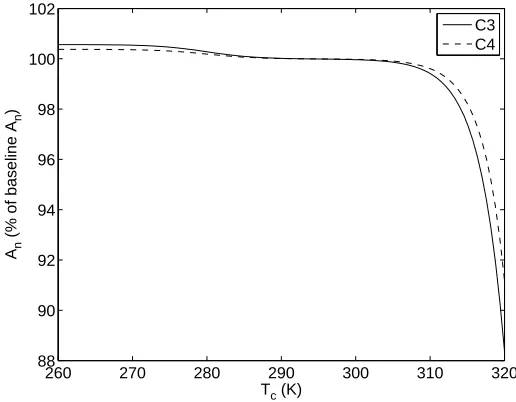
2.3.2 Canopy Temperature Tc
Tc is used in the calculation of mesophyllic conductance (gm), which yields no restrictions to the possible range of Tc. We examine the regionTc = [265,320] as shown in Figure 2.3.
2600 270 280 290 300 310 320 50
100 150 200 250 300 350 400
Ts (K)
An
(% of baseline A
n
)
C3 C4
Figure 2.2: Response ofAn to surface temperature Ts.
260 270 280 290 300 310 320 88
90 92 94 96 98 100 102
Tc (K)
An
(% of baseline A
n
)
C3 C4
2.3.3 Ambient Temperature Ta
Ta is used in the calculation of the virtual ambient temperatureTva and the forced convection leaf boundary layer conductancegbf c. Both of these variables impact the value of leaf boundary layer conductance gb. As with the preceding other two temperature parameters, we examine the range Ta= [260,320] as shown in Figure 2.4.
Compared to the sensitivity exhibited to the other temperature parametersTsandTc,Anis not as reactive to the value of Ta. HereAnincreases with increasing Ta. For C3, this is nearly a linear increase where for C4 it appears to be approaching an asymptote.
270 280 290 300 310 97
97.5 98 98.5 99 99.5 100 100.5 101 101.5 102
Ta (K)
An
(% of baseline A
n
)
C3 C4
Figure 2.4: Response ofAn to ambient temperatureTa.
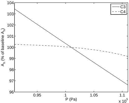
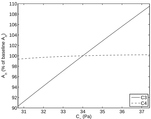
2.3.4 Surface Pressure P
Standard air pressure at sea level, approximately 1010 millibars or 101 kPa, indicates a typical value for P. Note that P is included in the calculation of the boundary layer conductance terms gbf c and gbf r, stomatal conductance gs, net assimilation rate Am, CO2 partial pressure
at the leaf surface Cs, and in intercellular spaces Ci for both models. Additionally, the PEP-Carboxylase limitation ws for C4 species also depends on P.
0.95 1 1.05 1.1 x 10⁵ 96
97 98 99 100 101 102 103 104
P (Pa)
An
(% of baseline A
n
)
C3 C4
Figure 2.5: Response ofAn to surface pressureP.
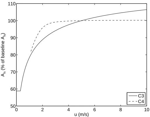
2.3.5 Wind Speed u
Typical values foru can range from 0 - 10 m/s. The wind speed is only used in the calculation of gbf c in the model. The leaf boundary layer conductance gb is defined as the maximum of the free (gbf r) and forced (gbf c) conditions. Of all the parameters involved in the calculation of these two terms, the only instance wheregb is defined bygbf r is when the value ofu is less than 0.4 m/s. Therefore, when u <0.4, gb is defined by gbf r which is independent ofu; hence there is no change inAn in this range of u.
0 2 4 6 8 10 50
60 70 80 90 100 110
u (m/s)
An
(% of baseline A
n
)
C3 C4
Figure 2.6: Response ofAn to wind speedu.
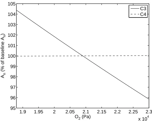
2.3.6 Oxygen Availability in Leaf Cells O2
The utilized value for O2in several published models [21, 29, 47, 59] ranges from 20.9 to 21 kPa.
Figure 2.7 illustrates the sensitivity ofAnto perturbing the baseline value of 2.09×104 Pa by 10%.
As expected, the C4 species exhibits nearly no change in An when varying this parameter. Recall that only the C3 species is impacted by photorespiration and therefore increased oxygen levels produce more oxygenase activity effectively inhibiting photosynthesis. This effect is clearly illustrated in Figure 2.7 where increasing levels of O2 cause a reduction in An and reciprocally decreasing levels of O2 allow An to increase.
2.3.7 Photosynthetically Active Radiation P AR
Photosynthetically active radiation is typically 45-65% net radiation depending on cloud cover [43]. On a non-cloudy day, net radiation is around 600 W/m2, but on any given day can be
between 400 and 1000 W/m2. To convert from the energy units, W/m2, to the quantum units employed in the model, mol m−2 s−1, we use the relationship
E = hc
λ (2.64)
where E = energy per photon (Joules), h = Planck’s constant = 6.63 × 10⁻³⁴ J · s,
pho-1.9 1.95 2 2.05 2.1 2.15 2.2 2.25 2.3 x 10⁴ 95
96 97 98 99 100 101 102 103 104 105
O2 (Pa)
An
(% of baseline A
n
)
C3 C4
Figure 2.7: Response ofAn to oxygen availability in leaf cells O2.
tons = 6.02 ×10²³ photons (Avagadro’s number). Assuming daylight has a wavelength of
approximately 550 nm, which is midway in the range for P AR of 400-700 nm, then we have
1
E = hcλ = 550×10
−9
m (6.63×10⁻³⁴J
·s)(3×10⁸m/s) = 2.7652×10
18 photons per Joule. Therefore, in daylight,
we have 2.7652×10¹⁸
photons/Joule
6.02×10²³photons/mol = 4.6×10⁻⁶ mol/Joule. Since 1 Watt = 1 J/s, we can simply
convert any value from W/m2 to mol m−2 s−1 by multiplying by 4.6×10⁻⁶. Thus we examine
the range of PAR associated with 0.45·400 = 180 and 0.65·1000 = 650 W/m2, or 8×10⁻⁴ to
3×10⁻³ mol m−2 s−1.
P AR is used in the calculation of the light limiting factorwe ofAg for both the C3 and C4 species, although the species require different formulations; see (2.22) and (2.28). Figure 2.8 illustrates that An is not remarkably sensitive to the amount of light. This implies that the remaining two limiting mechanisms, wc and ws, are more critical and that plants are not fully utilizing the light available.
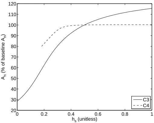
2.3.8 Relative Humidity at Leaf Surface hs
Normal atmospheric values forhsfall between 0.2 and 0.99. We chose to examine the full range of possibility forhs, from 0 to 1, as illustrated in Figure 2.9. Relative humidity is used in the model to relate stomatal conductance, net photosynthesis rate, and the CO2 concentration at
1 1.5 2 2.5 3 x 10⁻³ 96
97 98 99 100 101 102 103
PAR (mol m−2 s−1)
An
(% of baseline A
n
)
C3 C4
Figure 2.8: Response ofAn to photosynthetically active radiationP AR.
0 0.2 0.4 0.6 0.8 1
20 30 40 50 60 70 80 90 100 110 120
hs (unitless)
An
(% of baseline A
n
)
C3 C4
![Table 2.2: Model parameters from Niyogi et al. [48].](https://thumb-us.123doks.com/thumbv2/123dok_us/1696953.1214952/28.612.100.530.101.626/table-model-parameters-from-niyogi-al.webp)