_____________________________________________________________________________________________________
*Corresponding author: E-mail: [email protected];
www.sciencedomain.org
Automated Glaucoma Detection Using Support
Vector Machine Classification Method
Abhishek Dey
1and Samir K. Bandyopadhyay
1*1
Department of Computer Science and Engineering, University of Calcutta, Kolkata, India.
Authors’ contributions
This work was carried out in collaboration between both authors. Both authors read and approved the final manuscript.
Article Information
DOI: 10.9734/BJMMR/2016/19617
Editor(s):
(1) Ian Dooley, Limerick Regional Hospital, Republic of Ireland. (2)Pradeep Venkatesh, Professor, Ophthalmology, All India Institute of Medical Sciences, New Delhi, India. (3)Chan Shen, Department of Biostatistics, MD Anderson Cancer Center, University of Texas, USA.
Reviewers:
(1) Italo Giuffre, Catholic University of Roma, Italy. (2)Gabor Nemeth, University of Debrecen, Hungary. (3)Anonymous, University of Eastern Finland, Finland. Complete Peer review History:http://sciencedomain.org/review-history/12010
Received 19th June 2015 Accepted 28th September 2015 Published 29th October 2015
ABSTRACT
Glaucoma is an eye disease that can result in blindness if it is not detected and treated in proper time. Increased intraocular pressure (IOP) of the fluid in the eye often causes glaucoma. Glaucoma is the second leading cause of blindness in the world and is called as the “Silent Thief of Sight”. Optical Coherence Tomography (OCT) and Heidelberg Retinal Tomography (HRT) techniques for detecting glaucoma is very expensive. A method to diagnose glaucoma using digital fundus images is presented in this paper. The aim of our proposed method is to apply image processing techniques on the digital fundus images of the eye for analysing glaucomatous eye and normal eye. Images pre-processing techniques such as noise removal and contrast enhancement, Principal Component Analysis (PCA) method for feature extraction and Support Vector Machine (SVM) method for image classification are used in the proposed method. All these techniques are implemented via MATLAB which provides variety of options for image processing that enable us to extract the required features and information from the images.
Keywords: Glaucoma; histogram features; segmentation; feature extraction; computer aided diagnosis; principal component analysis; support vector machine.
1. INTRODUCTION
The eyes, with which we view the world, are the most complex, delicate and sensitive organs in our human body. They are responsible for four fifth of all the information our brain receives. Glaucoma is the term applied to a group of eye diseases that gradually result in loss of vision by permanently damaging the optic nerve, the nerve that transmits visual images to the brain [1]. Eduard Jaeger (1854) described glaucoma as the silent thief of sight which is a specific optic nerve disease with the progressive break down of nerve fibers [2]. The eye is filled with a fluid (aqueous), which has a stable pressure called intraocular pressure (IOP). This fluid is continuously formed within the eye and is also simultaneously drained out to maintain a stable IOP. IOP is increased due to the blockage of the normal outflow mechanism. This situation damages the optic nerve of the eye. This elevation in IOP is generally associated with the development of glaucoma, although additional factors may be also responsible in its development. In some cases, glaucoma may occur in the presence of normal eye pressure. This form of glaucoma is believed to be caused by poor regulation of blood flow to the optic nerve. Glaucoma is the diagnosis given to a group of ocular conditions that contribute to the loss of retinal nerve fibres with a corresponding loss of vision. Glaucoma therefore is a disease of the optic nerve, the nerve bundle which connects the eye to the brain and relays the visual signal [2].
There are two main types of glaucoma: "open-angle" and "closed-"open-angle" (or "angle closure") glaucoma [2]. Open-angle chronic glaucoma is painless, develops slowly over time. It often shows no symptoms until the disease has progressed significantly. It is treated with either glaucoma medication to lower the pressure, or with various pressure-reducing glaucoma surgeries. Unlike open-angle glaucoma closed-angle glaucoma, is characterized by sudden ocular pain, redness, nausea and vomiting, and other symptoms resulting from a sudden spike in IOP. It is treated as an ocular emergency. The iridocorneal angle between the iris and the cornea is used to differentiate open angle glaucoma and closed angle glaucoma [2].
As lost capabilities of the optic nerve cannot be recovered, it is necessary to detect glaucoma at
an early stage. Subsequent treatment is essential for affected patients to preserve their vision. Manual analysis of the eye is time consuming and the accuracy of the parameter measurements also varies with different clinicians. Optical Coherence Tomography (OCT) and Heidelberg Retinal Tomography (HRT) are used in glaucoma detection but the cost of these methods is very high [3]. As an alternative, many ophthalmologists use fundus cameras to diagnose glaucoma [4]. Image processing techniques allow to extract the features that can provide useful information to diagnose glaucoma.
This paper presents a novel method for to detect glaucoma using digital fundus images. At first, the images of eye fundus are pre-processed. Then, Principal Component Analysis (PCA) method is used for extracting features from pre-processed images. After PCA, the modified images are fed into a Support Vector Machine (SVM) classifier for training purpose. The performance of the classifier is tested by cross validation approach. Now, the classifier can distinguish between a normal eye fundus and a glaucoma affected eye fundus up to a certain level of accuracy.
2. LITERATURE REVIEW
Several studies are reported in literature for detection of optic disk and detection and classification of glaucoma.
In year 2006, Kevin Noronha performed a work, "Enhancement of retinal fundus Image to highlight the features for detection of abnormal eyes" [5]. Different techniques that are used to detect main features of retinal fundus images such as fovea, optic disk, exudates and blood vessels are specified in this work. Author finds the brightest part of the fundus and applies Hough transform to determine the optic disk and its centre.
In year 2008, S. Sekhar performed a work," Automated localization of retinal optic disk using hough transform" [7]. In this work, the proposed methodology consists of two steps: in the first step, region of interest (ROI) is found by image by means of morphological processing, and in the second step, optic disk is detected using the Hough transform.
In year 2010, Zhuo Zhang performed a work," ORIGA-light: An Online Retinal Fundus Image Database for Glaucoma Analysis and Research" [8]. Author present an online dataset, ORIGA-light, which aims to share clinical retinal images with the public. Author had updated the system continuously with more clinically verified ground-truth images. The proposed method focuses on optic disk and cup segmentation.
In year 2010, Vahabi Z proposed," The new approach to Automatic detection of Optic Disc from non-dilated retinal images" [9]. Author describes a new filtering approach like Sobel edge detection, Texture Analysis, Intensity and Template matching to detect Optic Disc. The proposed algorithm is applied in wavelet domain on 150 images of Messidor dataset.
In year 2011, Zafer Yavuz performed a work," Retinal Blood Vessel Segmentation Using Gabor Filter and Tophat Transform" [10]. In this paper, Author gave a method for retinal blood vessels segmentation by applying firstly Gabor filter to enhance blood vessels and then applying top-hat transform. Later on, the output is converted to binary image with p-tile thresholding.
In year 2012, Nilan jan Dey performed a work," Optical Cup to Disc Ratio Measurement for Glaucoma Diagnosis Using Harris Corner" [11]. In this paper, CDR is determined using Harris Corner. Harris comer detector measures the local changes of the signal with patches shifted in different directions by a small amount. It is based on the local auto-correlation function of a signal.
In year 2012, R. Geetha Ramani performed a work," Automatic Prediction of Diabetic Retinopathy and Glaucoma through Retinal Image Analysis and Data Mining Techniques" [12]. This paper proposed a novel approach for automatic disease detection. Retinal image analysis and data mining techniques are used to accurately categorize the retinal images as either normal, Diabetic Retinopathy and Glaucoma affected.
In year 2013, S. Sri Abirami and S. J Grace Shoba proposed “Glaucoma Images Classification Using Fuzzy Min-Max Neural Network Based On Data-Core” [13]. In this method, the Optical Coherence Tomography (OCT) images are preprocessed which includes colour conversion, resizing and pruning before it is given as input for classification. This classification technique uses Fuzzy min-max neural network algorithm.
In year 2014, Sheeba O., Jithin George, Rajin P. K., Nisha Thomas, and Sherin George proposed “Glaucoma Detection Using Artificial Neural Network” [14]. Here neural network is trained to recognize the parameters for the detection of different stages of the disease. The neuron model has been developed using feed forward back propagation network.
3. PROPOSED METHODOLOGY
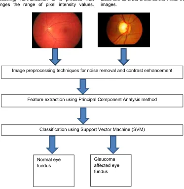
The block diagram of the proposed system for the detection of glaucoma is shown in Fig. 1. The various steps in our proposed method i.e image pre-processing, feature extraction and dimensionality reduction and image classification are detailed in the following section
3.1 Image Pre-processing
Retinal images are acquired with a digital fundus camera which captures the illumination reflected from the retinal surface. Despite controlled conditions, many retinal images suffer from non-uniform illumination given by several factors: the curved surface of the retina, pupil dilation (highly variable among patients), or presence of diseases among others [14]. The curved retinal surface and the geometrical configuration of the light source and camera lead to a poorly illuminated peripheral part of the retina with respect to the central part. Pre-processing is the step taken before the major image processing task. The problem here is to perform some basic tasks in order to render the resulting image more suitable for the job to follow [14]. In this case it may involve enhancing the contrast, removing noise. Pre-processing can dramatically improve the performance of image processing methods like Image transform, Segmentation, Feature extraction and disease detection. Several techniques have been used to enhance retinal images. Pre-processing also eliminates disease independent variations from the input image [14].
At first, some preprocessing tasks are required to be done on the input images as mentioned above. This includes normalizing the images, colour conversion from RGB to grayscale, resizing the images, removal of noise from the images and contrast adjustment for improving image quality. In our method, instead of preprocessing some particular regions of images, entire images are preprocessed before feature extraction and classification tasks.
3.1.1 Normalization
In our method, the original raw input images are normalized in the range [0, 1], resized to 256 X 256 and converted to grayscale before noise removal and contrast improvement. In image processing, normalization is a process that changes the range of pixel intensity values.
Applications include photographs with poor contrast due to glare, for example. Normalization is sometimes called contrast stretching or histogram stretching. In more general fields of data processing, such as digital signal processing, it is referred to as dynamic range expansion. The motivation is to achieve consistency in dynamic range for a set of data, signals, or images and also Principal Component Analysis method cannot be applied on un-normalized images.
3.1.2 Colour conversion
Then the normalized RGB images are converted to grayscale images as grayscale images are easier to be operated upon for preprocessing tasks like contrast enhancement than true colour images.
Fig. 1. Proposed design for detection of Glaucoma
Image preprocessing techniques for noise removal and contrast enhancement
Feature extraction using Principal Component Analysis method
Classification using Support Vector Machine (SVM)
Normal eye fundus
3.1.3 Resizing
After that, the grayscale images are resized to 256 X 256 as SVM classifier cannot be trained using images of different dimensions. Also, resizing images improves efficiency in implementation and reduces runtime overhead.
3.1.4 Noise removal
Image noise is random variation of brightness or colour information in images, and is usually an aspect of electronic noise. It can be produced by the sensor and circuitry of a scanner or digital camera. Noise reduction is the process of removing noise from the input image. Our goal is to remove the noise from the image in such a way that the original image is discernible [14]. We have used two -dimensional Gaussian Filter for noise removal. A Gaussian filter smooths an image by calculating weighted averages in a filter box. It is more effective in smoothing images than normal mean filter.
3.1.5 Improvement of image contrast
After noise removal, Adaptive Histogram Equalization technique is used for improving image contrast. Histogram equalization increases the dynamic range of the histogram of an image and intensity value of pixels in the input image. The output image contains a uniform distribution of intensities and increased contrast of an image than the original image. Adaptive Histogram Equalization differs from ordinary histogram equalization in the respect that the adaptive method computes several histograms, each corresponding to a distinct section of the image, and uses them to redistribute the lightness values of the image. It is therefore suitable for improving the local contrast [14]. This step also removes the non-uniform background which may be due to non-uniform illumination or variation in the pigment colour of eye.
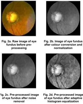
Fig. 2: (a), (b), (c) and (d) show an eye fundus image and pre-processed images after colour conversion and normalization, noise removal and adaptive histogram equalization.
Fig. 2a. Raw image of eye fundus before
pre-processing
Fig. 2b. Image of eye fundus after colour conversion and
normalization
Fig. 2c. Pre-processed image of eye fundus after noise
removal
Fig. 2d. Pre-processed image of eye fundus after adaptive
3.2 Feature Extraction Using Principal Component Analysis Method
In this paper, the normalizing features were extracted by using Principal Component Analysis (PCA) method and the features were fed to the SVM classifier. Principal Component Analysis (PCA) is a mathematical procedure that uses an orthogonal transformation to convert a set of observations of possibly correlated variables into a set of values of linearly uncorrelated variables called principal components. This transformation is defined in such a way that the first principal component has the largest possible variance (that is, accounts for as much of the variability in the data as possible), and each succeeding component in turn has the highest variance possible under the constraint that it is orthogonal to (i.e., uncorrelated with) the preceding components. The principal components are orthogonal because they are the eigenvectors of the covariance matrix, which is symmetric. PCA is sensitive to the relative scaling of the original variables. PCA is a powerful tool for analysing data because it is a simple, non-parametric method of extracting relevant information from confusing data sets. The other main advantage of PCA is when identifying patterns in the compress data (or by reducing the number of dimension) the information loss is very less. The number of principal components is less than or equal to the number of original variables.
After pre-processing step, we get pre-processed input images with size 256 X 256. These images are basically 256 X 256 matrices with normalized pixel values where rows correspond to observations and columns correspond to samples or data dimensions. The steps of PCA are as follows:
Step 1: Subtract the mean
For PCA to work properly, we have to subtract the mean from each of the data dimensions. The mean subtracted is the average across each dimension. This produces a data set whose mean is zero.
Step 2: Calculate the covariance matrix
In probability theory and statistics, covariance is a measure of how much two random variables change together. If the greater values of one variable mainly correspond with the greater values of the other variable, and the same holds for the smaller values, i.e., the variables tend to
show similar behaviour, the covariance is positive. In the opposite case, when the greater values of one variable mainly correspond to the smaller values of the other, i.e., the variables tend to show opposite behaviour, the covariance is negative. The sign of the covariance therefore shows the tendency in the linear relationship between the variables. A covariance matrix is a matrix whose element in the i, j position is the covariance between the i th and j th elements of a random vector (that is, of a vector of random variables). Intuitively, the covariance matrix generalizes the notion of variance to multiple dimensions. For n dimensional image data, the covariance matrix will be n Xn.
Step 3: Calculate the eigenvectors and eigenvalues of the covariance matrix
Since the covariance matrix is square, we can calculate the eigenvectors and eigenvalues for this matrix. These are important as it gives useful information about the data.
Step 4: Choosing components and forming a feature vector
we want to keep from the list of eigenvectors, and forming a matrix with these eigenvectors in the columns.
Feature Vector = (eig1 eig2 eig3…eign)
Step 5: Deriving the new data set
This is the final step in PCA, and is also the easiest. Once we have chosen the components (eigenvectors) that we wish to keep in our data and formed a feature vector, we simply take the transpose of the vector and multiply it on the left of the original data set, transposed.
FinalData= RowFeatureVector x RowDataAdjust
where RowFeatureVector is the matrix with the eigenvectors in the columns transposed so that the eigenvectors are now in the rows, with the most significant eigenvector at the top, and RowDataAdjust is the mean-adjusted data transposed, ie. the data items are in each column, with each row holding a separate dimension. It will give us the original data solely in terms of the vectors we chose. Basically we have transformed our data so that it is expressed in terms of the patterns between them. Now the columns of the matrix FinalData are separate features which are linearly uncorrelated.
In order to get the original data back, we can use the equation shows below:
RowDataAdjust = RowFeatureVector-1 X FinalData
RowDataAdjust= RowFeatureVectorT X FinalData
RowOriginalData = (RowFeatureVectorT X FinalData) + OriginalMean
3.3 Classification using Support Vector Machine (SVM)
A classification task usually involves separating data into training and testing sets. Each instance in the training set contains one target value (i.e. the class labels) and several attributes (i.e. the features or observed variables).
We have used support vector machine (SVM) classifier, a supervised learning model, for
classifying normal eye fundus from glaucoma affected eye fundus. The goal of SVM is to produce a model (based on the training data) which predicts the target values of the test data given only the test data attributes [15]. In our case, the input image matrices modified after applying preprocessing techniques and PCA in the previous steps serve as test data.
SVM is designed to separate of a set of training images into two different classes, (x1, y1), (x2, y2),…(xn, yn) where xi in Rd, d-dimensional feature space, and yi in {-1,+1}, the class label, with i=1..n. SVM builds the optimal separating hyper planes based on a kernel function (K). All images, of which feature vector lies on one side of the hyper plane, belong to class -1 and the others are belong to class +1 [16].
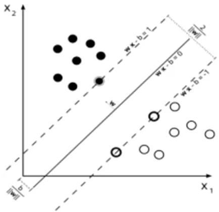
As we can see from Fig. 3, H3 does not separate the two classes while H1 separate the two class with a small margin, only H2 gives a maximum margin between two classes, therefor it’s the right hyper plane used by support vector machine.
If the data of various classes can be separated as in Fig. 3, then the linear SVM is used. Otherwise if the data of the classes cannot be separated, then the non-linear SVM classifier is used. However, instead of defining a function for the hyper plane itself; we define the margin in between the two classes. From Fig. 4, we can see that the position of our hyper plane depends on the value of w where w is the (not necessarily normalized) normal vector to the hyper plane.
More formally, linear SVM classifier function can be defined as,
f(x) = wT x + b (1)
such that for each training sample xi the function gives f(xi)> 0 for yi = +1, and f(xi) < 0 for yi = -1. In other words, training samples of two different classes are separated by the hyperplane f(x) = wT x + b = 0, where w is weight vector and normal to hyperplane, b is bias or threshold and xi is the data point.
The nonlinear SVM classifier is defined as,
f(x) = wT ϕ(x) + b (2)
functions. A kernel function on two samples, represented as feature vectors in some input space, is defined as k(xi, xj) = ϕ(xi)T ϕ(xj), ϕ is the feature vector. Most commonly used kernels are:
Linear kernel: k(xi, xj) = xiTxj (3)
Polynomial Kernel: k(xi, xj) = (γxiTxj + r)d, (4)
where r is a free parameter trading off the influence of higher-order versus lower-order
terms in the polynomial, d is the degree of the polynomial, slope γ>0
RBF Kernel: k(xi, xj) = exp (−‖ ‖
σ ), (5)
where σ>0 is an adjustable free parameter; higher σ means that the kernel is a "flatter" Gaussian and so the decision boundary is "smoother"; lower σ makes it a "sharper" peak, and so the decision boundary is more flexible
Fig. 3. Separating hyper planes between two classes
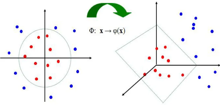
Fig. 5. Support vector machine kernel trick for non-linear classification
Sigmoid Kernel: k(xi, xj) = tanh(γxi T
xj + r), (6)
where γ is the slope and r is the intercept constant. It is also called Hyperbolic Tangent kernel or Multilayer Perceptron kernel.
Fig. 5 shows by applying SVM kernel trick (as explained above) a non-linear classifier can be transformed into a linear separating hyper plane in higher dimensional feature space [17].
SVM is a binary linear classifier but it can be extended for multiclass problems also. However, our problem is a two class prediction problem where normal healthy eye fundus images will belong to one class (say positive class) and glaucoma affected eye fundus images will belong to another class (say negative class). We have used RBF kernel as kernel function taking parameter σ=1.5.
4. EXPERIMENTAL RESULTS
In our method, 100 fundus images which consist of 50 normal fundus images and 50 glaucoma affected fundus images are used. All the image pre-processing, feature extraction and SVM classification techniques in our proposed method are simulated in MATLAB 8.1 (R2013a) and run on an Intel(R) Core(TM) Quad CPU-Q 8200 PC with 8-GB memory.
These images are pre-processed through a series of steps as described in section 4.1. Then these pre-processed images are modified by Principal Component Analysis for feature extraction. After that, these modified images are
fed into a Support Vector Machine classifier for training purpose.
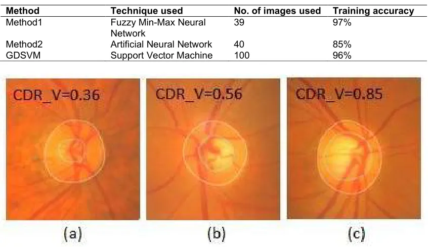
In this work, we consider three classes: non-glaucoma, glaucoma suspect and glaucoma cases.
Generally, the cup-to-disc ratio (CDRV) in vertical is the main indicator to analyze the development of glaucoma. When the CDRV is increased gradually, it also means that the size of the optic cup becomes larger. According to the ophthalmologist’s suggestion when CDRV is higher than 0.6 is considered as glaucoma as shown in Fig. 6.c. When CDRV is approximately between 0.4 and 0.6, it is in the suspect range of glaucoma as described in Fig.6.b. Finally, Fig. 6 shows the comparison of CDRV in each stage.
number of observations), the k-fold validation is exactly the leave-one-out cross-validation.
We have taken k=10. 90 images are used for training and 10 images are used for testing each time. This process is repeated 10 times using different sessions of the test data each time. Performance of the classifier can be tested and evaluated by the following parameters:
Accuracy rate = Correctly classified samples / Classified samples
Sensitivity = Correctly classified positive samples / True positive samples
Specificity = Correctly classified negative samples / True negative samples
Positive Predictive Accuracy = Correctly classified positive samples / Positive classified samples
Negative Predictive Accuracy = Correctly classified negative samples / Negative classified samples
Here, sample denotes input images used for training the classifier.
In our work, after cross validation trained SVM classifier has accuracy rate 96%, sensitivity 100%, specificity 92%, positive predictive accuracy 92.59% and negative predictive accuracy 100%.
After training, we have tested the performance of the trained classifier on 50 eye fundus images (20 normal and 30 glaucoma affected) which were not in the trained set of input images. The SVM classifier can successfully classify this test set with accuracy rate 86%, sensitivity 100%, specificity 65%, positive predictive accuracy 81.08% and negative predictive accuracy 100%.
We have collected fundus images of eye from Susrut Eye Foundation & Research Centre, Kolkata. These are all real world images verified by eye specialists. Comparison of our proposed method with other recent methods is shown below:
We name methods used in references [13,14] as Method 1, Method 2. Our method is named as GDSVM
It can be observed that, our method GDSVM is optimal compared to other recent methods with respect to number of images and also accuracy. We have used more images for classification and testing than Method 1 and Method 2.
Method Technique used No. of images used Training accuracy
Method1 Fuzzy Min-Max Neural Network
39 97%
Method2 Artificial Neural Network 40 85%
GDSVM Support Vector Machine 100 96%
5. CONCLUSION
In this paper, our aim is to develop a model which can classify glaucomatous eye fundus images from healthy eye fundus with high accuracy. We have used Support Vector Machine classifier for this purpose. Only a few minutes of runtime are necessary for training the SVM classifier. Hence, the computational efficiency of SVM is great. SVM is advantageous as only a small training set is needed to provide very good results because only the support vectors are of importance during training. For these reasons, SVM tends to perform better than other supervised learning methods. We have developed our model using RBF kernel. Before PCA some statistical features can be extracted from fundus images for gaining more efficiency in the classification method. Our proposed method is designed to help the doctors in their decision making process for detecting glaucoma.
CONSENT
It is not applicable.
ETHICAL APPROVAL
It is not applicable.
COMPETING INTERESTS
Authors have declared that no competing interests exist.
REFERENCES
1. ManjulaSri Rayudu. Review of image processing techniques for automatic detection of eye diseases. 2012 Sixth International Conference on Sensing Technology (ICST) 978-1-4673-2248-5/12 ©2012 IEEE.
2. A tutorial on Principal Components Analysis, Lindsay I Smith; 2002.
3. Rüdiger Bock, Jörg Meier, László G Nyúl, Joachim Hornegger, Georg Michelson.
Glaucoma risk index: Automated glaucoma detection from color fundus images. Medical Image Analysis. 2010;14(3):471– 481.
4. Rathinam S, Selvarajan S. Comparison of image preprocessing techniques on fundus images for early diagnosis of glaucoma. International Journal of Scientific & Engineering Research. 2013;4(12). ISSN 2229-5518.
5. Kevin Noronha, Jagadish Nayak, Bhat SN. Enhancement of retinal fundus Image to highlight the features for detection of abnormal eyes. TENCON 2006. 2006 IEEE Region 10 Conference.
6. Sangyeol Lee, Michael D Abr`amoff, Joseph M Reinhardt. Validation of retinal image registration algorithms by a projective imaging distortion model. 29th Annual International Conference of the IEEE EMBS Cité Internationale, Lyon, France August 23-26, 2007.
7. Sekhar S. Automated localisation of retinal optic disk using hough transform. Department of Electrical Engineering and Electronics, University of Liverpool, UK; 2008.
8. Zhuo Zhang. ORIGA-light: An online retinal fundus image database for glaucoma analysis and research. 32nd Annual International Conference of the IEEE EMBSBuenos Aires, Argentina, August 31 - September 4, 2010.
9. Vahabi Z. The new approach to automatic detection of optic disc from non-dilated retinal images. Proceedings of the 17th Iranian Conference of Biomedical Engineering (ICBME2010), 3-4 November 2010.
10. Zafer Yavuz. Retinal blood vessel segmentation using gabor filter and tophat transform; 2011. IEEE 19th Signal Processing and Communications Applications Conference (SIU 2011) 978-1-4577-0463-511/11 ©2011 IEEE
11. Nilan jan Dey. Optical cup to disc ratio measurement for glaucoma diagnosis using harris corner, ICCCNT12.
12. Geetha Ramani R. Automatic prediction of diabetic retinopathy and glaucoma through retinal image analysis and data mining techniques; 2012.
13. Sri Abirami S, Grace Shoba SJ. Glaucoma images classification using Fuzzy Min-Max neural network based on data-core. International Journal of Science and Modern Engineering (IJISME). 2013;1(7). ISSN: 2319-6386,
14. Sheeba O, Jithin George, Rajin PK, Nisha Thomas, Sherin George. Glaucoma detection using artificial neural network. IACSIT International Journal of Engineering and Technology. 2014;6(2). 15. A Practical Guide to Support Vector
Computer Science National Taiwan University, Taipei 106, Taiwan, Available:http://www.csie.ntu.edu.tw/~cjlin 16. Le Hoang Thai, Tran Son Hai, Nguyen
Thanh Thuy. Image classification using support vector machine and artificial neural network. I.J. Information Technology and Computer Science. 2012;5:32-38.
17. Reddy SVG, Thammi Reddy K, Valli Kumari V. An SVM based approach to
breast cancer classification using RBF and polynomial kernel functions with varying arguments. International Journal of Computer Science and Information Technologies. 2014;5(4):5901-5904. 18. Kavita Choudhary, Sonia Wadhwa.
Glaucoma detection using cross validation algorithm. Fourth International Conference on Advanced Computing & Communication Technologies; IEEE. 2014;478-482. _________________________________________________________________________________
© 2016 Dey and Bandyopadhyay; This is an Open Access article distributed under the terms of the Creative Commons Attribution License (http://creativecommons.org/licenses/by/4.0), which permits unrestricted use, distribution, and reproduction in any medium, provided the original work is properly cited.
Peer-review history: