R E S E A R C H
Open Access
A pest management model with state
feedback control
Qiong Liu
1*, Lizhuang Huang
2and Lansun Chen
3*Correspondence: [email protected] 1College of Mathematics and Computer Science, Qinzhou University, Qinzhou, 535000, People’s Republic of China Full list of author information is available at the end of the article
Abstract
In this paper, research of a class of state feedback control model which is mainly used in crop pests management, with Bendixson-Dulac discriminance, proves that this model has an unique and globally stable positive equilibrium under the weak time-delay kernel function. Also, we adopt the subsequent function method in the ordinary differential equation of the geometric theory to prove that a sufficient condition holds for the existence of an order one period solution in the system. At the same time, it also proves that the periodic solution is asymptotically stable.
Keywords: pest management; successor function; periodic solution of order one; Bendixson-Dulac discriminance
1 Introduction
Crop is an essential part of the human food resources for sustainable development. There-fore, crop yields directly affect social and economic development as well as social stability. In recent years, in order to improve the yield of crops and meet the needs of human sur-vival, people used a lot of pesticide [–] to keep pest down to improve the yield of crops, but the excessive use of pesticides will make the pests drug-resistant, pollute the environ-ment, and also do some harm to people and animals. So how to reduce the effect caused by pests but doing no harm to the living environment of human beings and animals is an issue which has attracted extensive concern of ecologists and biomathematics researchers. In [–], the authors established a specific pest management model based on the actual problem and analyzed pest management issues by the corresponding mathematical the-ory. We will explore the feasibility of the crop pest management from the mathematical model of state feedback control in this paper.
In recent years, the research on the pest management has made many achievements. It can be classified into two categories: one is using farm chemicals, but this method will strengthen the drug resistance of the pests and it is harmful to the environment. The other is adopting a biological treatment [–] such as taking advantage of the characteristics of inter-restriction between the beneficial organisms and pests, it can effectively maintain a long-term balance with the effects on the food chain. The latter treatment is a more extensive pest treatment at present. It is a better measure to control pest by cultivating natural enemies of the pests to destroy pests, but the delivery of natural enemies and use of pesticides are not regular, depending on the amount of pests. Therefore, we must give full consideration to the natural inhibition in the agricultural ecological system. Meanwhile,
delivery of a natural enemy and use of pesticides are transient phenomena, which we call a pulse phenomenon. In biological control, we do not need to reduce the amount of pests to zero, but we usually control the indicator of the state of an illness under a certain indicator, and this cannot only boost the yields of crops, but also it has no negative influences on the environment. We call the indicator of the state of an illness the economic index (EI), also known as the control index.
The infinite delay logistic model of classic single species is expressed as
dx(t)
Here,x(t) is the population density att,a,b,care positive constants,aexpresses the innate capacity of increase,b,cexpress the density restriction coefficient, the integral kernelk
is continuous and meets∞k(s)ds= and∞sk(s)ds< +∞. In system (), whenb= , one has a so-called non-pure time delay, and when b= , it is called a pure time delay. Corresponding to system (), Fengde Chen [] also put forward the model of an infinite delay logarithmic population:
In practical pest management, we do not periodically use the pesticide before we deter-mine the pesticide. So, on the basis of system (), this paper studies the impulsive state feedback control with continuous weak delay logarithm population,
Under the condition of a weak integral kernel, the given specific integral kernelk(t–s) =
e–d(t–s), we make a transformation, assumingu(t) =lnx(t),v(t) =–t∞e–d(t–s)lnx(s)ds; then
System () turns into the following system:
⎧
Among them,urefers to crop pest density,vrefers to the hysteresis effect of the pest,lnh
factors,dis positive constant, which refers to the parameters of the normal distribution,
∞
e
sds= , <β< is the ratio of spraying pesticide pests.
2 Preparation
First of all the related definition is given []. Consider the state impulsive differential equations
dx
dt =f(x,y), dy
dt =g(x,y), (x,y)∈M(x,y),
x=α(x,y), y=β(x,y), (x,y) /∈M(x,y). ()
Here,M(x,y) andN(x,y) are straight lines or curves on the planeR(x,y),M(x,y) is the
pulse set,N(x,y) is the phase set,ϕ(M) =N, system () is called a constituted power sys-tem. It is a straight line or curve inR+
={(x,y)∈R|x≥,y≥}.
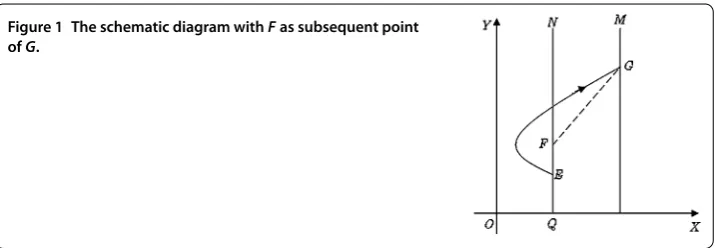
Definition . AssumeMis the pulse set,N is the phase set, andMandN are both straight lines, as shown in Figure . Assume the coordinate of the point of intersectionQ
ofNandxisO, and the distance betweenEandQon the lineNis denotedc. The path line through the pointEintersects with the pulse set at pointG, the phase point of the point
Gin the phase setNisF, and the coordinate isd. We define pointFto be the subsequent point of the pointEand the successor function of the pointEisG(E) =d–c.
For convenience in our discussion, the following definitions are used in this article in terms of the subsequent function.
Definition . The point of intersection between the path lineLand the phase setu= ( –β)lnhisN, the point of intersection between the path lineLand the pulse setu=lnh
is impulsing and itsvcoordinate difference to the phase pointNon the phase setu=
( –β)lnh,G(N) =Nv–Nv.
Lemma .[] The subsequent function G(E)is continuous.
Lemma . Assume in the continuous dynamical system(X,),there are two points,x, xin pulse phase set,to make the successor functions,G(x) > ,G(x) < ,then there must be a point E between xand xto make G(E) = .Thus,there must be a periodic solution of order one through E between xand x.
Lemma .(Similar Poincaré norm) Assume the periodic solutions of T - in the following
The path asymptotically stable.Assume the multiplier umeets|u|< .Here,
u=
Lemma .(Bendixson-Dulac discriminance []) Consider the system dx
maintains a constant value and it is zero all the time in any subdomain,then system()
has no closed trajectory in D.
3 Existence and stability of the periodic solution of order one for the impulsive differential equation of plant diseases and insect pests
In system (), ifβ= , then we will obtain a mathematical model for control of the class-A crops diseases and insect pests without pulse,
du
dt =a–bu–cv, dv
dt =u–dv.
()
Ifβ> , then system () obeys the following.
Lemma . The positive equilibrium point of system()E(u∗,v∗) =E( ad
As a result the system’s variational matrix is
So, the characteristic equation in theE(u∗,v∗) is
λ+b c
– λ+d
= (λ+b)(λ+d) +c= .
Namely,λ+λ(b+d) +bd+c= .
We obtainλ,=
–(b+d)±√(b+d)–(bd+c)
, in whichb,d,care all constant.
Assume=T– D= (b+d)– (bd+c),T= –(b+d),D=bd+c.
() When= ,T< ,D> , the two characteristic rootsλ=λis a multiple negative
real root, at this point, the solution curve tends to equilibrium, called the degenerate node.
() When> ,T< ,D> , the two characteristic rootsλ=λis a pair of negative
real roots, at this point, the solution curve tends to equilibrium, called the stable node.
() When< ,T< ,D> , the two characteristic rootsλ,λhave real parts and
they are negative conjugate complex roots, at this point, the solution curve tends to equilibrium, and the equilibrium is called a focal point.
From the above analysis, we can see the characteristic roots shall be two conjugate com-plex roots of which two are negative or a pair with a negative real part and this shows that the positive equilibrium pointE(u∗,v∗)Tis locally stable. It can also be noticed that on the
Rplane, constantly
∂P ∂u+
∂Q
∂v = –(b+d) < .
From Lemma . we know that on the whole plane the system has no limit cycle, and because there is only a balance in the system, so all the path lines takeE(u∗,v∗)Tas the limit set, the system is stable at the balance pointE(u∗,v∗)T and on the planeR. It is hereby
proved.
When the positive constantsb,c,dmeet (b+d)< (bd+c), the positive equilibrium is
a stability focal point, namely when the real part of the two characteristic rootsλ,λare
negative conjugate complex roots, of whichv=a–bclnhis the intersection pointD(lnh,v)
between the pulse setu=lnhand the line dudt = , and whenh≥, we have the following theorem.
Theorem .
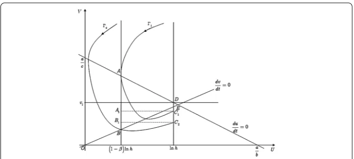
() If the pulse set <lnh≤c+adbd,then system()has a periodic solution of the order one. () If the pulse setlnh> ad
c+bd> ,there are the following four conditions: (i) Whencv<v,cv<v,system()has a periodic solution of order one.
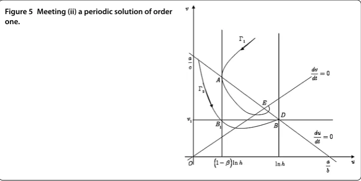
(ii) If the subsequent pointBoverlapsB,the other path linehas no intersection
point with the pulse set,then system()has a periodic solution of order one. (iii) Ifcv<v,the system path linehas no intersection point with the pulse set
lnh,then system()has no periodic solution of order one,but for anyt,we have
v(t)≤v+bβclnh.
(iv) If the system path lines,have no intersection point with the pulse setlnh,
then system()has no periodic solution of order one,but,for anyt,we have
Figure 2 When lnh<c+bdad , there is a periodic solution of order one in the diagram.
Proof () Assume the pulse setlnh≤u∗= ad
c+bd, namelyv>v∗= a
c+bd, like Figure . From the equationua–=bulnh–,cv= ,we obtainv=a–bclnh.
From the equationu= ( –β)lnh,
a–bu–cv= ,we obtainv= a–bu
c =
a–b(–β)lnh c =v+
bβlnh c .
So, the system trajectorypassing through the pointA(( –β)lnh,v+bβclnh) in the
phase set ( –β)lnhintersects with the pulse setlnhatC(lnh,cv), and this results in a pulse action in the phase setu= ( –β)lnh, the phase point isA(( –β)lnh,cv), obviously,
the vertical coordinate of the pointAis less than that of the pointA, we have
G(A) =Av–Av=cv– v+ clnhβ
c
< .
Assumeu= ( –β)lnhintersects with dvdt = at B(( –β)lnh,(–β)dlnh), then select the system path linepassing the pointBintersects with the pulse setlnhatC(lnh,cv) and
results in a pulse action in the phase setu= ( –β)lnhatB(( –β)lnh,cv). And because
the path line’s segmental arc is below the straight line dvdt = , so on the segmental
arcBCwe havedvdt > , namelyvmonotonically increases, with the nature of monotonic
function we can obtaincv> (–β)dlnh, so there is a successor functionG(B) =Bv–Bv=
cv–(–β)dlnh> .
According to Lemma ., in the phase setu= ( –β)lnh, there must bePwhich meets
Bv<Pv<Av, to makeG(P) =Pv–Pv= , namely there is a periodic solution of order one in system ().
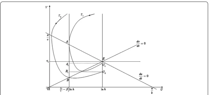
With the same method, we can prove that when lnh= c+adbd, system () has a peri-odic solution of order , like Figure . Select the path lineintersecting with the pulse
set ( –β)lnhatA(( –β)lnh,bβclnh), and intersecting with the pulse set atC(lnh,cv),
the phase point after the pulse is A(( –β)lnh,cv), as the path line is below the
du
dt = , the segmental arc above the dv
dt = has dv
dt < , namely thevmonotonically de-creases, therefore, the vertical coordinate of the point A is less than that of the point A, we have G(A) =Av–Av=cv– (v + cβclnh) < . In the same way, select the path
line intersecting with the pulse set ( –β)lnh at the point B(( –β)lnh,(–β)dlnh)
and intersecting with the pulse set at C(lnh,cv), the phase point after the pulse is
B(( –β)lnh,cv), and because the segmental arcBC of the path line is below the
Figure 3 When lnh= ad
c+bd, there is a periodic solution of order one in the diagram.
Figure 4 Meeting (i) a periodic solution of order one in the diagram.
the monotonic function, we can obtaincv>(–β)dlnh, so the successor function ofBobeys
G(B) =Bv–Bv=cv–(–β)dlnh> .
According to Lemma ., in the phase setu= ( –β)lnh, there must be∃P(P), this meets
Bv<Pv<Av, and it enablesG(P) =Pv–Pv= , namely there is a periodic solution of order one in system ().
() If the pulse set obeyslnh>cad+bd, under this condition, there are four situations as follows.
When ( –β)lnh<u∗= ad
c+bd<lnh, namelyv<v∗= a c+bd<v+
cβlnh c .
(i) Ifcv<v,cv<v, then system () has a periodic solution of order one, as shown
in Figure . Assume the intersection point between the pulse set lnh and the line du
dt =a–bu–cv= is D, the coordinate of D is solved by the following equation set:
u=lnh,
We can obtain
u=lnh,
v=a–bclnh.
So for pointD(lnh,a–blnh
c ), we can select the path line passing the intersection point
Abetween the phase set ( –β)lnhand the line du
dt = , the coordinate of the pointA isA(( –β)lnh,v+bβclnh), intersecting with the pulse set atC and acts on the phase
set with the pulse action, the phase point is A, the segmental arc of the path line,
dv
dt < , is below the line du
dt = and above dv
dt = , so thev(t) monotonically decreases. Therefore, according to the nature of the monotonic function, we can obtain a verti-cal coordinate of the point A that is greater than that of the point A, namely Av>
Av, so the successor function ofAisG(A) =Av–Av< . In the same way, select the path line passing the intersection pointBbetween the phase set ( –β)lnhand the
line dudt = , intersecting with the pulse set at C, the phase point of the
correspond-ing phase set after the pulse isB, because the segmental arcBC of the path lineis
below the line dvdt = , dvdt > , we can thus know thev(t) monotonically increases, with the nature of the monotonic function, we can obtain vertical coordinate of the point
B is less than that of the pointB, namely Bv>Bv, so the successor function of Bis
G(B) =Bv–Bv> .
According to Lemma ., in the phase set u= ( –β)lnh, Pmust meetBv<Pv<Av, and this enablesG(P) =Pv–Pv= , namely there is a periodic solution of order one in system ().
(ii) If the path line passes the and the pointBof the phase set, intersects with the
pointBin the pulse set (the pointBcoincidesD), through the pulse action, the subsequent point ofBcoincidesB, that is, theparts monotonically increase and decrease on both
sides of the line dv
dt = are equal, and with Lemma ., we must haveG(B) = , at the same time, the other path linehas no intersection point with the pulse set, then there
is a periodic solution of order one in system (). This is shown in Figure .
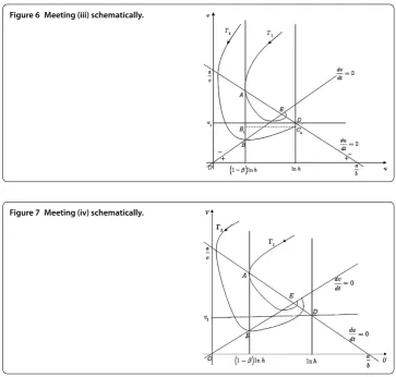
(iii) Ifcv<v, the system’s path linehas no intersection points with the pulse setlnh,
then there is no periodic solution of order one in system (), but for anyt, we havev(t)≤
v+bβclnh, as shown in Figure . Due to considering the actual biological significance, the
path line does not intersect with the pulse line, indicating there are not many pests, with
Figure 6 Meeting (iii) schematically.
Figure 7 Meeting (iv) schematically.
little harm to crops, so it cannot be controlled, that is to say, we can always find a path line cut in the phase setA, and the path line is fully near the pulse set, but it has no intersection with the pulse to constitute one biggest attraction domain, all of the path lines eventually arrive at the traction domain, with no intersection with pulse set, we do not need pulse control, pest populations in this area cannot meet the monitoring limit. Therefore, there is no periodic solution of order one. But any constituted attraction domain hasv(t)≤
v+blnchβ for anyt.
(iv) If the system path lines,have no intersection point with pulse setlnh, then
there is no periodic solution of order one in system (), but for anyt, we havev(t)≤v+
blnhβ
c , as shown in Figure . There is no intersection point between the path line and the pulse set, not meeting the definition of the periodic solution of order one, so there is no periodic solution of order one. Considering the actual biological significance, the analysis
is the same as (iii). Theorem . is proved.
When <h< , namely the pulse setlnh< < ad
c+bd, then there is no periodic solution of order one in system (). This case has no real biological meaning, so it is no longer considered.
Proof By system () we can obtain
Takeinto the following formula:
4 Conclusion
This paper focuses on an ecosystem model of class-A plant diseases and insect pests to analyze the stability of the equilibrium of the model; it discusses the sufficient condition for the existence of a periodic solution of order one of the system, and at the same time, it also proves the conditions under which the periodic solution is asymptotically stable. On the basis of the model, it carried on the qualitative and quantitate analysis, to draw some conclusions under certain conditions. That is to say, there is a periodic solution of order one in this paper and it is asymptotically stable, under this situation the number of pest is controlled to a certain extent, it will be finally controlled to a be a periodic solution of order one in which the once-occurring pulse finally controls the number of pest. It can be seen from the article that, according to the different crop growth cycle, the observation and record of the quantity of pests in production can help the crop-dusting to control pest populations, so as to protect crops.
Competing interests
The authors declare that they have no competing interests.
Authors’ contributions
QL carried out the main part of this article, LC corrected the manuscript, LH brought forward some suggestions on this article. All authors have read and approved the final manuscript.
Author details
1College of Mathematics and Computer Science, Qinzhou University, Qinzhou, 535000, People’s Republic of China. 2College of Mathematics and Information Science, Guangxi University, Nanning, 530004, People’s Republic of China. 3Academy of Mathematics and System Sciences, Chinese Academy of Sciences, Beijing, 100080, People’s Republic of China.
Authors’ information
Qiong Liu, female, Qinzhou University College of Mathematics and Computer Science Professor. Master research circle tutor.
Acknowledgements
This work was supported by National Natural Science Foundation of China (10861003) and The Research Fund of Guangxi Higher Education of China (ZD2014137), Natural Science Foundation of Guangxi Province (No. 2016GXNSFAA380102).
Received: 6 May 2016 Accepted: 28 September 2016
References
1. Wang, ZL: The main plant diseases and insect pests and prevention and cure technology of balsam pear. Qinghai Pop. Agric. Sci. (4),30(2006)
2. Tang, SY, Xiao, YN: Single Population Biological Power System. Science Press, Beijing (2008) 3. Wang, MX: Chemical pesticide and environmental hormone. Rural Ecol. Environ.15(4), 35-37 (1999) 4. Zhao, YF: The research progress of pesticide residues in food analysis. Foreign Med.25(3), 173-177 (1998) 5. Wang, K: Random Biological Mathematical Model. Science Press, Beijing (2010)
6. Wei, CJ, Liu, Q: Pest management virus infection model. Syst. Sci. Math.30(8), 1059-1069 (2010)
7. Fu, JB, Chen, LS: Pollution-free pest management strategy of mathematics research. Math. Practice Underst.41(2), 144-150 (2011)
8. Jiao, JJ, Chen, LS: A pest management SI model with impulsive control concerned. J. Biomath.22(3), 385-394 (2007) 9. Chen, HD: Impulse on the beneficial insects chemical control pest management model. J. Sun Yat-sen Univ. Natur.
Sci. Ed.49(3), 8-11 (2010)
10. Chen, YP, Liu, ZJ: Extinction and permanence of pest management SI model with twice impulses and Nonlinear incidence rate. J. Biomath.24(4), 609-619 (2009)
11. DeBach, P, Rosen, D: Biological Control by Natural Enemies. Cambridge University Press, Cambridge (1991) 12. Grasman, J, van Herwaarden, OA, Hemerik, L, van Lenteren, JC: A two-component model of host-parasitoid
interactions: determination of the size of inundative release of parasitoids in biological pest control. Math. Biosci.
169(2), 207-216 (2001)
13. Kidd, NAC, Jervis, MA: Population dynamics. In: Insect Natural Enemies. Springer, London (1996)
14. Chen, FD: Periodic solutions and almost periodic solutions for a delay multispecies logarithmic population model. Appl. Math. Comput.171(2), 760-770 (2005)
15. Chen, LS: Pest control and geometric theory of semi-continuous dynamical system. J. Beihua Univ. Nat. Sci.,12(1), 1-9 (2011)
16. Liu, Q: The mathematical model of the red squirrel protection. Syst. Sci. Math.33(9), 1083-1092 (2013)