Search | Preprints

Scaling Group Analysis of Mixed Bioconvective Flow in Nanofluid with Presence of Slips, MHD and Chemical Reactions

Md Faisal Md Basir1*_{, M.J. Uddin}2 _{and Ahmad Izani Md Ismail}1*

1_{School of Mathematical Sciences, Universiti Sains Malaysia,11800, Penang, Malaysia.} 2_{Mathematics Department, American International University-Bangladesh, Kuratoli, Dhaka 1229,}

Bangladesh.

*Corresponding Email: [email protected]

*Co-author Email: [email protected],[email protected]

Abstract

Bioconvective flows have attracted attention in recent years due to actual and potential applications. In this paper, we consider a steady and laminar convective MHD flow of a nanofluid with heat, mass and microorganism transfer with a heat source/sink present. In addition, we assume there exists a first order chemical reaction. The governing partial differential equations (PDEs) are reduced to ordinary differential equations (ODEs) using the scaling group transformation and the associated boundary value problem is then solved. The influences of selected governing parameters on the dimensionless velocity, temperature, nanoparticle concentration, density of motile microorganisms, skin friction, heat transfer, mass transfer, and motile microorganism density rates are computed and discussed.

Keywords: Bioconvection, Magnetohydrodynamics, Scaling group of transformations, Slip boundary conditions, Chemical reaction

1. Introduction

Bioconvection is a process where microorganisms (denser than water) swim in an upward manner on average causing the upper surface of the suspension to be very dense (due to the accumulation of microorganisms), become unstable and sink. Resilient microorganisms swimming upwards maintain this bioconvection pattern [1–3]. Several studies have been conducted to explain the mechanism of directional motion of the different types of microorganisms [4–7]. It has been found that the resultant large-scale motion of fluid containing self-propelling motile microorganisms enhances mixing, preventing nanoparticle agglomeration in nanofluids [8–10]. Bioconvection control is essential for certain biological and biotechnological processes. For instance, controlling populations of plankton

communities in the ocean and separating vigorous swimming subpopulation of microorganisms in laboratory experiments [11]. “Taxes” are the response to the movements. “Chemotaxis” means that the swimming is due to chemical gradients whereas “phototaxis” means the movement along or opposite the direction of light, “gravitaxis” refers to swimming under gravitational field, “gyrotaxis” refers to swimming which results from the balance between the physical torques generated by viscous drag and gravity operating on an asymmetrical distribution of mass within the microorganism [12]. Finally, “oxytaxis” refers to swimming due to oxygen gradient.

Kuznetsov [13] developed a theory of nanofluid bioconvection in a horizontal porous layer heated from below. Non-oscillatory and oscillatory convections were investigated. The obtained results indicate that the effect of microorganisms on the stability of the suspension may depend on the value of bioconvection Péclet number. Water-based nanofluid with heat and mass transfer along a wavy surface with the presence of motile gyrotactic microorganisms were theoretically investigated by [14,15]. The Buongiorno model with no-slip boundary conditions was employed.

2. Mathematical Formulations of the Problem

Consider a two-dimensional, steady, viscous incompressible, hydromagnetic laminar mixed convective boundary layer slip flow of a nanofluid over a stationary plate with microorganism. The effect of heat generation/absorption and chemical reaction are considered. The configuration of the problem is shown in Fig. 1. Within the boundary layer, the fluid temperature, the nanoparticle volume friction and the density of motile microorganisms are denoted by T, C and n respectively. At the wall, the temperature, nanoparticle volume friction and density of motile microorganisms are represented byT_w,C_w and ,n_w(respectively) and far away from the wall they are denoted by T_,C_ and n_, (respectively). In addition, there are four different boundary layers formed near the plate includes (i) velocity boundary layer, (ii) concentration boundary layer, temperature boundary layer and microorganism’s boundary layer (In general in Figure 1, they are not the same). The surface of the plate is subjected to boundary conditions with multiple slip conditions. The velocity components along thexandydirections are denoted by uand vrespectively. A magnetic field of variable field strength B x

L    

  is applied in the positive direction of the

y

-axis. We have incorporated first order chemical reaction in the concentration equation. We also included heat generation/absorption in the energy equation. By using these assumptions, the following five field equations representing the conservation of mass, momentum, thermal energy, nanoparticle volume friction and density of motile microorganisms are [20].

0,

V

   (1)

 

2 _,

DV

p V F

Dt _ _         _{ } (2)





2 _, p T B D x Q

L _{T T} c

DT

T D T C T T

D t   T 

                            

  (3)

 

2 T 2





_,

B

D DC

D C T

Dt T

x

K C C

L       _{ }      _  

  (4)





2

_,

c

n

bW

Dn

n C

D

n

Dt





C

   



Where D V Dt t      

is the material derivative, i j, 2

x y

 

   

 

 

: Laplacian operator. t is the

dimensional time, F F_buoF_mag(F_buo=buoyancy force,F_mag=magnetic force). By applying boundary layer approximations, we obtain:

0, u v x y  _ _

  (6)





















2 2 2 1 1 ( ), ( ) e c e

f p f

c e

f _{m f} f

du

u u u

u v K u

x y dx y

x B

C g T T g C C _L

u K u n n g





 







_{ }

_



      _{ }   _  _{ }          _{    }  _{ }         

  (7)

2 2

2 ( ),

T

p B

D

T T T T C T

u v D T T

x y y y y T

L y x Q c                       _{ }  

     _  _   (8)

2 2

2 2

(

),

T B

D

C

C

C

T

x

u

v

D

k

C C

x

y

y

T

_

y

L





_



_



_



_

 

_

 









 

(9) 2 2 . c m w bW

n n C n

u v n D

x y C C_ y y y

      _  _   _          _ _  _{ } _  (10)

The relevant amended boundary conditions are [21],

1 1

1

1 , 0, , ,

at 0,

, , , as ,

w w

w

c e

u

u N v T T C C

y

n n

x x T x C

D E

L L y L y

F y

x

u K u T T C C n n y

L x n L y



         _   _           _   _              _{ }                  _{   }           (11)

where u_eis the dimensional external fluid velocity, _f is the ambient fluid density,



is the

pressure, b is the chemotaxis constant, W_cis the maximum cell swimming speed,  is the thermal

diffusivity of the fluid,

( )

( )

p f

c

c









is the ratio of heat capacities, Q x L

 

 

  is the variable heat

generation/absorption, k x L

   

  is the variable reaction rate, 1

x N

L

   

  is the velocity slip factor,

1 x D L    

  is the variable thermal slip factor, 1

x E

L

   

  is the variable solutal slip factor, 1

x F

L

 

 

  is the

variable microorganism slip factor, D_B is the Brownian diffusion coefficient, D_T is the thermophoretic diffusion coefficient, D_m is the microorganisms diffusion coefficient. K_c is a constant and K_c0 represents for free convection flow while K_c 1 represents for mixed convective flow where thermal buoyancy, concentration buoyancy, motile microorganism’s buoyancy and pressure gradient terms are existing in the momentum equation. The following dimensionless variables are used in order to express the governing equations in dimensionless form,

1 4

1 1 1

2 4 2

,

,

,

,

,

,

,

,

(

)

c e

w

w w

e

K u

T T

x

yRa

uL

vL

x

y

u

v

u

L

L

T

T

Ra

Ra

Ra

x

n

C C

n n

C

C

n













     





























(12) where 3

(1

C g

)

_f

T L

Ra

 



 







_{is the Rayleigh number based on characteristic length which}

represents by

L

.

_{The stream function, defined as} u y



 

 and v x



  

 is introduced. The stream

function is applied in order to reduce the number of equations and number of independent variables. Hence, the transformed dimensionless momentum, energy, concentration and microorganism equations are as follows:





1 2

2 2 3

2 3 2 2

Pr

Pr

( )

,

e c e c e

du

K u

Nr

Rb

y x y

x y

dx

y

L

B x

K u

y

Ra







_

_

_











 

_

 

_

_



_

_

_

  

 











_



_



2

2 2

1 2

2

( ) 0,

p

L

Nb Nt Q x

y x x y y y y y

Ra c

 

 

 



_







    _  _ _   _   

       _ _   (14)

2 2 2

1

2 2

2

1 1 Nt L _{k x( ) 0,}

y x x y Le y Le Nb y

Ra        _   _  _  _  _{ }

      (15)

2 2

2 2

1

( ) 0,

Pe

y x x y Lb y y y Lb y

 

 



_



 





  _  _{  }  _  _  _

 

    _    _  (16)

and the corresponding boundary conditions becomes:

 

 

 

 

 

1 1 2 4 4 1 2 1 1 4 1 4 1 1

, 0, 1

1 1 at 0

, 0, 0,

,

0 as , . c e D y E Ra Ra

N x x

y L y x L

Ra Ra

x F x y

L L

K u x y

y y y            _{  }      _{  }  _{   }      _{ }   _{ }              _{ }  _{ }                   _{     }  (17)

The parameters involved in the above dimensionless Eqns. (13)-(17) are Prandtl number defined as

P r  , 

 buoyancy ratio parameter defined as

(

)

(1

)

p f f

C

Nr

C

T





 

  











, bioconvection Rayleigh

number defined as

(

)

,

(1

)

m f f

n

Rb

C

T

  

 

 











Brownian motion parameter defined as Nb DB C ,

 

thermophoresis parameter defined as _Nt D TT ,

T 

 _



 traditional Lewis number defined as , B Le

D 



bioconvection Lewis number, defined as , m Lb

D 

 bioconvection Péclet number defined as

c m bW D Pe



  and microorganisms concentration difference parameter defined as . w n n n      , T C

3. Applications of scaling group of transformations

It is often computationally expensive and complicated to directly solve the PDEs numerically[22]. A common approach is to convert the PDEs to ODEs and then solve the ODEs numerically. There are several types of group methods including (a) group method followed by boundary layer concepts, (b) deductive group method, (c) linear group of transformation, (d) scaling group of transformations and (e) Lie group analysis. Linear group of transformations is used to combine coordinates of x and y into a single independent variable called



and hence this transformation leads to ODEs. Scaling group transformation is one of the group methods where it is based on the invariance PDEs with relevant boundary conditions and hence used it to determine the similarity solution. Invariant solution of those equations is solved under an appropriate one (or more) parameter group of transformations [23,24]. Therefore, to carry out scaling group of transformations, we scale all independent and dependent variables as:

3 5

1 2 4

6 7 8 9

10 11 12 13 14

* * * * *

* * * *

1 1 1 1

* * * * 2* 2

1 1 1 1

: , , , , ,

, , , ,

, , , , ,

e e

x xe y ye e e e

e u u e N N e D D e

E E e F F e Q Qe k ke B B e

                                     (18)

Here  is a parameter and _i(i1, 2,...14) _{are all arbitrary real constant with not all zero. By} considering Eqs. (13)-(17) and boundary conditions Eqn. (13) in (*) form are:

1 2

* 2 * 2 3 *

* * *

* * * * *2 *3

* * * * * 2 * 2* * * Pr Pr ( ) , e c e c e du

K u Nr Rb

y x y x y dx y

L

B x K u

y Ra    _{  }         _  _{ }  _{    }            _  _    (19) 2

* * * * 2 * * * * 2

* 1

* * * * *2 * * *

2 , ) 0 ( p L

Nb Nt Q x

y x x y y y y y

Ra c

 

 



 



_





    _  _ _   _  _  

       _ _  (20)

* * * * 2 * 2 2

1

* * * * *2 *2

2 *

*

1 1

( ) 0,

Nt L

k x y x x y Le y Le Nb y

Ra

      _



  _  _  _  _{ }

      (21)

* * * * 2 * * * 2 *

*

* * * * *2 * * *2

1

( ) 0,

Pe

y x x y Lb y y y Lb y

 

 



_



 





  _  _{  }  _  _  _

 

    _    _  (22)

 

 

 

 

 

1 1

* ₄ 2 * * ₄ *

* *

1

* 2* * *

1 1 * * 4 4 * * * * * * * * * * 1 * * 1 1 *

, 0, 1 ,

1 , 1 at 0,

, 0, 0, 0 as .

c e

Ra Ra

N x x

y L y x L y

Ra Ra

x F x y

L y

D

E

y L

K u x y

y  _   _     _          _{  }  _{   }      _{ }   _{ }                _{ }  _{ }              _          (23)

Apply the scaling group transformation Eqn. (18) into Eqns. (19-23), the following relationship among the exponents are found to be invariants if i's are related as follows:

1 2 2 2 3 2 7 1 3 2 3 4 5 6 14 3 2 14 7,

              

               

1 2 3 4 2 2 4 2 2 4 5 2 2 2 4 4 2 12,

            

                 ₍₂₄₎

1 2 3 5 2 2 5 2 2 4 5 13,

         

           

1 2 3 6 2 2 5 6 2 2 5 6 5 2 ,2

           

             

and for boundary conditions:

2 8 9 10 11

4 5 6

,

0.

   



  















(25)

Relationship among  are:

1 2 2 8 9 10 11 3 2 4 5 6 7 2

12 13 14 2

4 ,

,

3 ,

0,

2 ,

2 .



    

 

   















  





  







 

(26)

Using Eqn. (26), transformations in Eqn. (18) become:

2 2 2 2

2 2 2 2 2 2

2

4 3 2

* * * * * * *

2 2

* * * * * *

1 1 1 1 1 1 1 1

2 2* : , , , , , , , , , , , , , . e e

x xe y ye e u u e

N N e D D e E E e F F e Q Qe k ke B Be                                      (27)

* * * * *

2 2 2

* * * *

2 1 1 2 1 1 2

* * * *

1 1 2 1 1 2 2 2

*

2

(1 4 ), (1 ), (1 3 ), (1 0), (1 0),

(1 0), (1 2 ), (1 ), (1 ),

(1 ), (1 ), (1 2 ), (1 2 ),

(1 2 ).

e e

x x y y

u u N N D D

E E F F Q Q k k

B B                                                (28)

Differential form of expression in (23) is:

(29)

From Eqn. (29), by solving one by one, the following transformations are obtained:

 

 

 

 

3 1 1

4 2 4

1 1

1 4

1 1 1 1 1

4 4 4 2 2

1 1 1 1 1 1

1 2 , ( ) , ( ), ( ), ( ), , , , , , ( ) , ( ) , ( ) , e y

f x u x N x N

x

D x D E x E F x F Q x x Q k x x k

B x x B







        

_                     

 ₍₃₀₎

where



is the similarity independent variable, f( )



,

 

( ),

 

( ) and

 

( ) are the dimensionless velocity, temperature, nanoparticle volume fraction functions and microorganisms, respectively.

 

N

1_ is the constant velocity slip factor,

 

D

1_ is the constant thermal slip factor,

 

E

1_ is the constant

mass slip factor,

 

F

1_ is the constant microorganism slip factor, Q0 is the constant heat

generation/absorption, k₀ is the constant reaction rate, B₀ is the constant magnetic field strength. By substituting Eqns. (30) into Eqns. (13) -(17), the similarity transformation equations obtained in term of ODEs are as follows:

2

3 1 1

''' '' ' ( ' ) 0,

4 Pr 2 Pr c 2 Pr Pr c

M

f  ff  f K   NrRb f K  (31)

2 '' ' ' ' ' , 4 0 3 c N

f b Nt Q

           (32)

3

'' '

4 '' 0,

Nt

Lef L

b eK

N

       (33)





3

'' ' ( ) '' ' ' 0,

4Lb f Pe

         (34)

1 1 1

1 1 1

1 1 1

4 3 0 0 0 2

1 ( ) 1 ( ) 1 ( )

.

2 ( ) 2 ( ) 2 ( )

e e

du dN dE dF

dx dy d d d d

x y u N E F

dQ x dk x dB x

Q x k x B x

   



         

and the boundary conditions become:

 

(0) 0,

'(0)

''(0), (0) 1

'(0), (0) 1

'(0),

(0) 1

'(0), '( )

_c

, ( ) ( )

0.

f

f

a f

b

c

d

f

K























 

 

 

 

     

(35)

Here, prime ( ) ' denotes ordinary differentiation with respect to



,

 

1 4 1

N Ra a

L





 is the velocity

slip parameter,

 

1 4 1

D Ra b

L





 is the thermal slip parameter,

 

1 4 1

E Ra c

L





 is the mass slip

parameter and

 

1 4 1

F Ra d

L





 is the microorganism slip parameter.

It is interesting to note that in the absence of the microorganism equation (Eqn. 34), magnetic field M, heat generation/absorption Q and chemical reaction K, our problem reduce to Uddin et al. [25] with the same similarity equations and boundary conditions.

4 Numerical solutions and validation

The set of nonlinear ODEs, Eqs. (31)-(34) with boundary conditions in Eq. (35) will be been solved numerically by using Runge-Kutta-Fehlberg fourth-fifth numerical method under Maple 2017 for various values of the flow controlling parameters. This method has been successfully applied by [26-30] and [31] and has generated accurate results. For the purpose of validation, the values of 



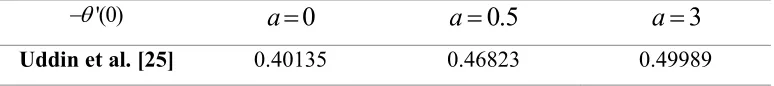
'(0) in present study was compared with the values of Uddin et al. [25] in Table 1. This table shows the comparison our result for values of 



'(0) with various a when ignore for microorganism equation,

0 c

M Q K b c   and _{Pr 1, NrNb Nt 10}5_.

Table 1: Values of 



'(0) in the case of ignore microorganism equation, thermal and iso-solutal plate (b c 0) with _{Pr 1, NrNb Nt 10}5 _{and 0.}

c M Q K 

'(0)





_a

_

₀

_a

_

_0.5

_a

_

₃

Khair and Bejan [32]

0.401 - -

Kuznetsov and Nield [33]

0.401 - -

Present 0.40103 0.46842 0.49989

5. Physical quantities

The quantities of practical interest in this study are the skin friction Cf, Nusselt number

Nu

,

Sherwood number

Sh

and the density number of motile microorganisms Nn_x defined as:

2, x w f e C u    , ( ) x w w xq Nu

k T T_



 x ( ),

m B w

xq Sh

D C C_

  ( ), n n w xq Nn

D n n_



 (36)

where _w,q_w, q_m and q_n represents the skin friction, surface heat flux, surface mass flux and the surface motile microorganism flux and defined by:

0 w y u y





  

 , w ₀

y T q k y _   

 , m B ₀

y C q D y _   

 , n B ₀.

y C q D y _   

 (37)

Substitute Eqns. (32) into (31) we obtain,

1/ 2

Re ''(0),

x

f x f

C  C  f 1/ 2

Re '(0),

x x

Nu   Nu  1/ 2

Re '(0),

x x

Sh   Sh 

1/ 2

Re '(0).

x x

Nn _  Nn_{ } ₍₃₈₎

6. Results and discussion

volume fraction transfers, and microorganisms transfer characteristics. For present study, the values are fixed at Pr=6.2, Nb=Nt=Rb=0.1, Pe=Lb=1, Le=3, 0.In this study we consider water-based nanofluids to be at (Pr=6.2) [36,37].

6.1

Effect of velocity slip (

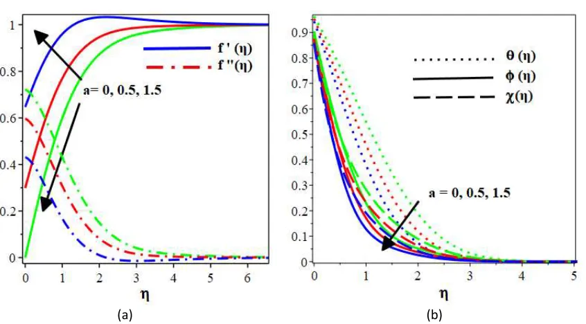
a)

Figure 2(a) shows profiles for dimensionless velocity and velocity gradient, while Figure 2(b) shows profiles for temperature, nanoparticle volume fraction/concentration and microorganism. It is observed from Figure 2(a) that the dimensionless velocity profiles increase with the increase of the velocity slip parameter. The fluid axial velocity at the plate surface is zero when the velocity slip parameter a=0 (no-slip case). The velocity of fluid at the environs of the plate has some non-zero values because of the velocity slip boundary condition at the plate, and therefore the thickness of the hydrodynamic boundary layer diminutions. Physically, as the velocity slip parameter increases, the entrance of the stagnant surface through the fluid purview subsides leading to a decrease in the hydrodynamics boundary layer – which was the same finding as that of Uddin et al. [38]. Rising of slip factor may be viewed as a miscommunication between the stationary plate and the moving fluid. In Figure 2(a), the velocity gradient decreases as the velocity slip increases due to the increase in the slip conditions at the stationary surface plate. This is because as slip conditions increase, the existence of the stationary plate will go unnoticed by the flow and hence the rate of heat transfer decreases. In Figure 2(b), dimensionless temperature is found to decrease with the growing of the velocity slip parameter. The physics behind it is that as the velocity slip parameter increases; more flow will infiltrate the boundary layer due to the slipping effect. As a result, hot plate heats more volumes of fluid and this pointers to the shrinkage in the temperature profiles. However, as velocity slip increases, effect on the dimensionless concentration and microorganism also slightly decreases.

6.2

Effect of thermal slip

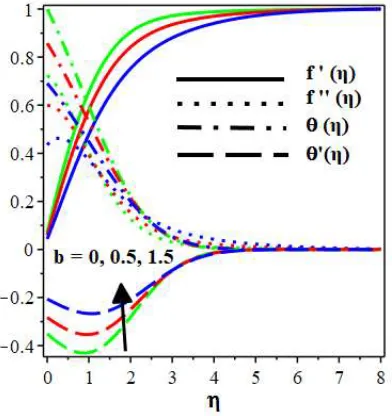
(b)

boundary condition relating to the dimensionless temperature to the temperature gradient in Equation (35) i.e.



(0) 1 b



'(0) shows that a positive increase in b,decreases the temperature gradient throughout the boundary layer regime. Notice that the thermal slip effect on the dimensionless concentration and microorganism is insignificant.

6.3

Effect of mass slip

(c)

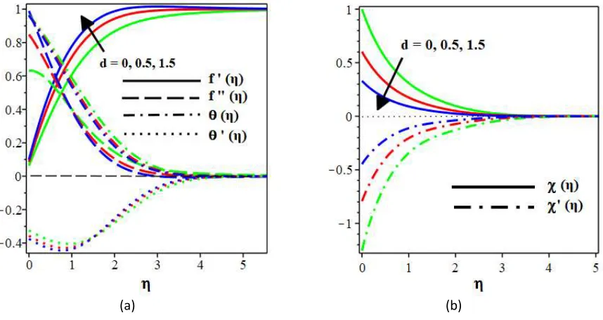
Figure 4 illustrates the influence of mass slip on the nanoparticle volume fraction, nanoparticle volume fraction gradient, microorganism and microorganism gradient. Nanoparticle volume fraction and microorganism profiles are found to decrease with an increase in mass slip parameter. In the case of iso-solutal plate (c0), nanoparticle volume fraction shows the maximum value. Nanoparticle volume fraction and microorganism gradients however increase with increasing mass slip. The decrease in nanoparticle volume fraction and microorganism concentration in the boundary layer results in enhanced migration of nanoparticles and microorganisms to the sheet surface, resulting in a boost of mass and microorganism transfer rates at the wall.

6.4

Effect of microorganisms slip

(d)

Figures 5(a)-(b) show representative profiles for dimensionless velocity, velocity gradient, temperature, temperature gradient, microorganism, and microorganism gradient. It is observed from Figure 5(b) that the microorganism profiles decrease with the increase of microorganism slip parameter. The fluid axial microorganism at the plate surface is maximum when the microorganism slip parameter is at d=0 (conventional no-slip case). It can be seen that for the no-slip case, the boundary condition and the microorganism parameter is between zero to one. The microorganism parameter approaches to zero asymptotically which means that the solution satisfies the graph obtained. In Figure 5(b) microorganism transfer rate however increases with increasing mass slip. A decrease in microorganism in the boundary layer results in enhanced migration of microorganism species to the sheet surface, resulting in a boost of microorganism transfer rates at the wall.

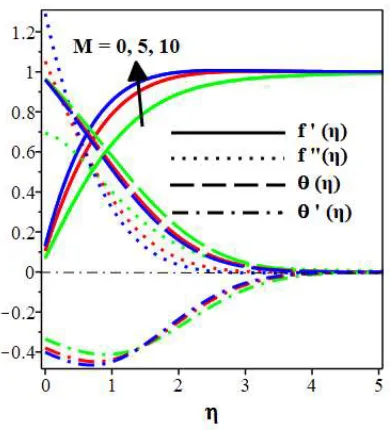
6.5

Effect of the magnetic field parameter (

M)

perpendicular to the wall. Therefore, in Figure 6, application of M tends to increase the movement of the fluid which increases the velocity near the surface and hence velocity gradient (shear stress) also increases. Meanwhile, temperature gradient decreases with the increasing of M. Also, notice that the value of f ' 1 and therefore magnetic field term will always enhance the velocity in momentum equation.

6.6

Effect of heat generation/absorption parameter (Q)

Figure 7(a) shows velocity and velocity gradient, Figure 7(b) illustrates temperature and temperature gradient, Figure 7(c) displays nanoparticles volume fraction and nanoparticles volume fraction gradient and Figure 7(d) portrays microorganism and microorganism gradient distribution for different values of heat source and sink Q. A rise value of heat source, Q from 0 to 0.4 clearly increases both in velocity and temperature. Physically, this situation occurs due to the increase of buoyancy force when heat is generated, inducing the flow rate to increase and hence increase the velocity profiles. In terms of temperature, Rajotia and Jat [39] found that the rising of internal heat generation/absorption parameter Q have the tendency to attribute the presence of an exponentially decaying internal heat generation/absorption to the flow system which results in an increase of the thermal boundary layer thickness. Therefore, higher value of internal heat generation/absorption parameter Q implies higher surface heat flux. Meanwhile, the concentration and microorganism show a decreasing trend as the heat generation/absorption, Q is increased.

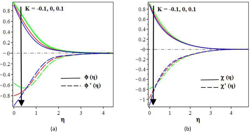
6.7

Effect of chemical reaction parameter (

K

)

For different values of the chemical reaction parameter K, the concentration and microorganism profiles are plotted in Figures 8(a)-(b). The size of fluid concentration decreases with the rise of chemical reaction parameter. A similar conclusion was also drawn by Idowu et al. [40]. It is obvious that as the values of chemical reaction K increases the concentration and microorganism distribution across the boundary layer decreases. The concentration boundary surfaces get thicker as the reaction parameter goes up.

Thus, it can be shown that an increase of velocity (momentum) slip parameter

a

_{increases heat}

transfer, temperature, nanoparticle volume fraction and microorganism rates but decreases skin friction/velocity gradient. Increasing thermal slip parameter

b

_{causes the numerical results to} decrease in skin friction, and temperature, nanoparticles volume friction and motile microorganism rates. Table 2 also shows increasing mass slip parameter

c

_{causes the numerical results to increase} in skin friction and heat transfer but decrease in nanoparticle volume fraction and microorganism rates. Next, increasing microorganism slip parameter

d

_{causes the numerical results to increase in} skin friction, heat transfer and nanoparticle transfer rates but decrease in microorganism transfer rate.

Meanwhile, increasing heat generation/absorption parameter Q_c causes the numerical results to decrease in heat transfer rate but increase in skin friction, motile microorganism and nanoparticles volume friction rates. Magnetic field effect

M

_{and heat generation/absorption parameter} Q_c however give variety of observations on heat transfer rate. It can be shown that increasing chemical reaction parameter

K

_{causes the numerical results to increase in skin friction, heat transfer, and} nanoparticles volume friction and motile microorganism rates.

7. Conclusion

MHD flow for steady two-dimensional laminar mixed convection boundary layer slip flow of nanofluid containing microorganisms past a vertical surface is investigated numerically. The momentum, temperature, concentration/nanoparticle volume fraction and microorganism equations are transformed into a set of ordinary differential equations and solved numerically. The convective process is controlled by the parameters , , , , , ,M Q K a b c d_c . We compared our numerical results with previous literature for some limiting cases. Based on the numerical results, the following summary is arrived where, we observed that:

 The skin friction number is increase with increasing mass slip parameter c, microorganism slip

reaction effect K _{but decreases with increasing velocity (momentum) slip parameter}

a

and

thermal slip parameter

b

.

 The local Nusselt number is increase with increasing thermal slip parameter

b

and heat generation/absorption effect Q_{c but decrease with increasing velocity (momentum) slip} parameter a mass slip parameter c microorganism slip parameter d, _{magnetic field effect} M

and chemical reaction effect K.

 The Sherwood number is increase with increasing thermal slip parameter

b

and mass slip parameter

c

_{but decrease with increasing velocity (momentum) slip parameter} a microorganism slip parameter ,d _{magnetic field effect} M, _{and chemical reaction effect} K _and

heat generation/absorption effect Qc.

 The number density of motile microorganism is increase with increasing thermal slip parameter ,

b mass slip parameter

c

_{and microorganism slip parameter}

d

but decreases with increasing velocity (momentum) slip parameter a _{magnetic field effect} M, _{and chemical reaction effect}

K _{and heat generation/absorption effect} Q_c.

8. Future Research

In future, this study may be extended for unsteady boundary value problems of various non-Newtonian fluids (such as power law fluid, micropolar fluids, viscoelastic fluids, second grade and third grade fluid) over horizontal surface of paraboloid of revolution [41,42]. Furthermore, bio-nano-particle geometric effects also certified more detailed analysis with different approach of numerical method i.e. a new pseudo-spectral technique called paired quasi-linearization method (PQLM) and these will be discovered [43].

Acknowledgement

References

1. Pedley TJ, Hill NA, Kessler JO. The growth of bioconvection patterns in a uniform suspension of gyrotactic micro-organisms. Journal of fluid mechanics. 1988; 195:223–237.

2. Ghorai S, Hill NA. Wavelengths of gyrotactic plumes in bioconvection. Bulletin of Mathematical Biology. 2000; 62:429–450.

3. Karimi A, Ardekani AM. Gyrotactic bioconvection at pycnoclines. Journal of Fluid Mechanics. 2013; 733:245–267.

4. Sharma YD, Kumar V. Overstability analysis of thermo-bioconvection saturating a porous medium in a suspension of gyrotactic microorganisms. Transport in Porous Media. 2011; 90:673– 685.

5. Kuznetsov A V. Nanofluid bioconvection in a horizontal fluid-saturated porous layer. journal of porous media. 2012; 15:11–27.

6. Shaw S, Sibanda P, Sutradhar A. Murthy PVSN. Magnetohydrodynamics and soret effects on bioconvection in a porous medium saturated with a nanofluid containing gyrotactic microorganisms. Journal of Heat Transfer. 2014; 136:52601.

7. Sheremet MA, Pop I. Thermo-Bioconvection in a square porous cavity filled by oxytactic microorganisms. Transport in Porous Media. 2014; 103:191–205.

9. Uddin MJ, Khan WA, Qureshi SR, Anwar Bég O. Bioconvection nanofluid slip flow past a wavy surface with applications in nano-biofuel cells. Chinese Journal of Physics. 2017; 55:2048–2063.

10. Mahdy A. Gyrotactic microorganisms mixed convection nanofluid flow along an isothermal vertical wedge in porous media. International Journal of Mechanical, Aerospace, Industrial, Mechatronic and Manufacturing Engineering. 2017; 11:840–850.

11. Kuznetsov A V. Nanofluid bioconvection: interaction of microorganisms oxytactic upswimming, nanoparticle distribution and heating/cooling from below. 2012; 26:291-230.

12. Kuznetsov A V. The onset of nanofluid bioconvection in a suspension containing both nanoparticles and gyrotactic microorganisms. International Communications in Heat and Mass Transfer. 2010; 37:1421–1425.

13. Kuznetsov A V. Nanofluid bioconvection: Interaction of microorganisms oxytactic upswimming, nanoparticle distribution, and heating/cooling from below. Theoretical and Computational Fluid Dynamics. 2012; 26:291–310.

14. Siddiqa S, Gul-e-Hina, Begum N, Saleem S, Hossain MA, Reddy Gorla RS. Numerical solutions of nanofluid bioconvection due to gyrotactic microorganisms along a vertical wavy cone. International Journal of Heat and Mass Transfer. 2016; 101:608–613.

15. Siddiqa S, Sulaiman M, Hossain MA, Islam S, Gorla RSR. Gyrotactic bioconvection flow of a nanofluid past a vertical wavy surface. International Journal of Thermal Sciences. 2016; 108:244– 250.

17. Koriko OK, Omowaye AJ, Sandeep N, Animasaun IL. Analysis of boundary layer formed on an upper horizontal surface of a paraboloid of revolution within nanofluid flow in the presence of thermophoresis and Brownian motion of 29nm CuO. International Journal of Mechanical Sciences. 2017;124-125:22-36.

18. Ibrahim SM. Effects of chemical reaction on dissipative radiative mhd flow through a porous medium over a nonisothermal stretching sheet. Journal of Industrial Mathematics. 2014; 2014:1-10.

19. Bhargava R, Sharma R, Beg OA. 2009. Oscillatory chemically-reacting mhd free convection heat and mass transfer in a porous medium with soret and dufour effects: Finite Element Modeling. Int. J. of Appl. Math and Mech. 2009; 5: 15-37.

20. Mutuku WN, Makinde OD. Hydromagnetic bioconvection of nanofluid over a permeable vertical plate due to gyrotactic microorganisms. Computers & Fluids. 2014; 95:88-97.

21. Kumar RVMSSK, Varma SVK. Multiple slips and thermal radiation effects on mhd boundary layer flow of a nanofluid through porous medium over a nonlinear permeable sheet with heat source and chemical reaction. Journal of Nanofluids. 2017; 6:48–58.

22. J.M. Hill, Differential Equations and Group Methods for Scientists and Engineers, CRS Press, Boca Raton, New York, 1992.

23. Thiagarajan M, Sivakumar PS, Srinivasan M, Lie Group Analysis for Thermal Radiation Effect on the MHD Flow over a Heated Stretching Sheet with Variable Viscosity, 2013; 1:1–9.

25. Uddin MA, Bég OA, Amin N, Hydromagnetic transport phenomena from a stretching or shrinking nonlinear nanomaterial sheet with Navier slip and convective heating: A model for bio-nano-materials processing, Journal of Magnetism and Magnetic Materials. 2014; 368:252–261.

26. Rana P, Bhargava R, Flow and heat transfer of a nanofluid over a nonlinearly stretching sheet: A numerical study, Communications in Nonlinear Science and Numerical Simulation. 2012; 17: 212– 226.

27. Khan WA, Makinde OD, MHD nanofluid bioconvection due to gyrotactic microorganisms over a convectively heat stretching sheet, International Journal of Thermal Sciences. 2014; 81:118–124.

28. Shalini J, Choudhary R. Dufour–Soret And Thermophoretic Effects On Magnetohydrodynamic Mixed Convection Casson Fluid Flow Over A Moving Wedge And Non-Uniform Heat Source/Sink. International Journal of Fluid Mechanics Research. 2018; 45:51-74.

29. Dhanai R, Rana P, Kumar L, Journal of the Taiwan Institute of Chemical Engineers Lie group analysis for bioconvection MHD slip flow and heat transfer of nanofluid over an inclined sheet: Multiple solutions, Journal of the Taiwan Institute of Chemical Engineers. 2016; 66: 283–291.

30. Aziz A, Khan WA, I. Pop, Free convection boundary layer flow past a horizontal flat plate embedded in porous medium filled by nanofluid containing gyrotactic microorganisms, International Journal of Thermal Sciences. 2012; 56:48–57.

32. Khair K, Bejan A. Mass transfer to natural convection boundary layer flow driven by heat transfer. Journal Heat Transfer. 1985; 107:979-81.

33. Kuznetsov A, Nield D. Natural convective boundary-layer flow of a nanofluid past a vertical plate: A revised model. International Journal of Thermal Sciences. 2014; 77:126-9.

34. Mahdy A. Natural convection boundary layer flow due to gyrotactic microorganisms about a vertical cone in porous media saturated by a nanofluid. Journal of the Brazilian Society of Mechanical Sciences and Engineering. 2016; 38:67-76.

35. Saini S, Sharma YD. Numerical study of nanofluid thermo-bioconvection containing gravitactic microorganisms in porous media:Effect of vertical throughflow. Advanced Powder Technology. 2018. doi: https://doi.org/10.1016/j.apt.2018.07.021.

36. Kuznetsov AV. Nanofluid bioconvection in water-based suspensions containing nanoparticles and oxytactic microorganisms: oscillatory instability. Nanoscale research letters. 2011; 6:100.

37. Mehryan SAM, Kashkooli FM, Soltani M, Raahemifar K. Fluid flow and heat transfer analysis of a nanofluid containing motile gyrotactic micro-organisms passing a nonlinear stretching vertical sheet in the presence of a non-uniform magnetic field: numerical approach,PLoS ONE. 2016; 1: e0157598.

39. Rajotia D, Jat R. Dual solutions of three dimensional MHD boundary layer flow and heat transfer due to an axisymmetric shrinking sheet with viscous dissipation and heat generation/absorption. Indian Journal of Pure and Applied Physics. 2014; 52:812-820.

40. Idowu AS, Dada MS, Jimoh A, Command KS, Heat And Mass Transfer Of Magnetohydrodynamic (MHD) And Dissipative Fluid Flow Past A Moving Vertical Porous Plate With Variable Suction, Mathematical Theory and Modeling. 2013; 3:80–103.

41. Koriko, OK, Omowaye AJ, Sandeep N, Animasaun, IL. Analysis of boundary layer formed on an upper horizontal surface of a paraboloid of revolution within nanofluid flow in the presence of thermophoresis and Brownian motion of 29 nm CuO. International Journal of Mechanical Sciences. 2017; 124:22-36.

42. Animasaun IL. 7nm alumina–water nanofluid flow within boundary layer formed on upper horizontal surface of paraboloid of revolution in the presence of quartic autocatalysis chemical reaction. Alexandria Engineering Journal. 2016; 55:2375-2389.

43. Motsa SS, Animasaun, IL. (2016). Paired quasi-linearization analysis of heat transfer in unsteady mixed convection nanofluid containing both nanoparticles and gyrotactic microorganisms due to impulsive motion. Journal of Heat Transfer. 2016; 138:114503.

List of Figures

Figure 1 : Schematic diagram of the problem

Figure 2 : Variation of velocity slip on the (a) dimensionless velocity (b) temperature, concentration, microorganism (c) gradient of temperature, concentration, microorganism

List of Table

(a) (b)

microorganism

Figure 5 : Variation of microorganisms slip on the (a) dimensionless velocity and temperature (b) microorganism

Figure 6 : Variation of magnetic field strength on the dimensionless velocity and temperature

Figure 7 : Variation of heat generation/absorption on the (a) dimensionless velocity (b) temperature, (c) concentration (d) microorganism

Figure 8 : Variation of chemical reaction on the (a) concentration (b) microorganism.

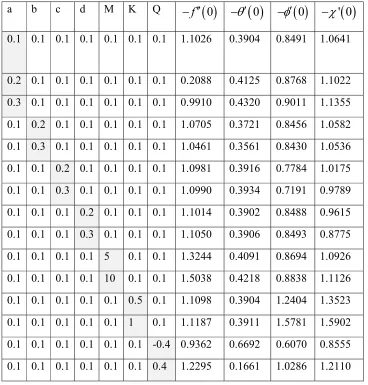
Table 2 : Results of skin friction, Nusselt, Sherwood numbers and density number of motile microorganisms for various values of parameters at Pr 6.8 ,

(c)

Figure 1: Variation of velocity slip on the (a) dimensionless velocity (b) temperature, concentration, microorganism (c) gradient of temperature, concentration, microorganism.

Figure 3: Variation of mass slip on the dimensionless concentration and microorganism.

(a) (b)

Figure 5: Variation of magnetic field strength on the dimensionless velocity and temperature.

(c) (d)

Figure 6: Variation of heat generation/absorption on the (a) dimensionless velocity (b) temperature, (c) concentration (d) microorganism.

(a) (b)

Table 2 Results of skin friction, Nusselt, Sherwood numbers and density number of motile microorganisms for various values of parameters at Pr 6.8 , Pe = Lb = Le = 0.5,Nb Nt0.1.

a b c d M K Q

_

_f

_

 

₀

_

_

_

 

₀

_

_

_

 

₀

_

_

_{' 0}

 

0.1 0.1 0.1 0.1 0.1 0.1 0.1 1.1026 0.3904 0.8491 1.0641

0.2 0.1 0.1 0.1 0.1 0.1 0.1 0.2088 0.4125 0.8768 1.1022 0.3 0.1 0.1 0.1 0.1 0.1 0.1 0.9910 0.4320 0.9011 1.1355 0.1 0.2 0.1 0.1 0.1 0.1 0.1 1.0705 0.3721 0.8456 1.0582 0.1 0.3 0.1 0.1 0.1 0.1 0.1 1.0461 0.3561 0.8430 1.0536 0.1 0.1 0.2 0.1 0.1 0.1 0.1 1.0981 0.3916 0.7784 1.0175 0.1 0.1 0.3 0.1 0.1 0.1 0.1 1.0990 0.3934 0.7191 0.9789 0.1 0.1 0.1 0.2 0.1 0.1 0.1 1.1014 0.3902 0.8488 0.9615 0.1 0.1 0.1 0.3 0.1 0.1 0.1 1.1050 0.3906 0.8493 0.8775 0.1 0.1 0.1 0.1 5 0.1 0.1 1.3244 0.4091 0.8694 1.0926 0.1 0.1 0.1 0.1 10 0.1 0.1 1.5038 0.4218 0.8838 1.1126 0.1 0.1 0.1 0.1 0.1 0.5 0.1 1.1098 0.3904 1.2404 1.3523 0.1 0.1 0.1 0.1 0.1 1 0.1 1.1187 0.3911 1.5781 1.5902 0.1 0.1 0.1 0.1 0.1 0.1 -0.4 0.9362 0.6692 0.6070 0.8555 0.1 0.1 0.1 0.1 0.1 0.1 0.4 1.2295 0.1661 1.0286 1.2110

Nomenclature

a velocity slip parameter

 

 

1 4 1 0

N Ra L



 

 _{ }

 

 

 

b

thermal slip parameter

 

1 4

1 0 _{( )}

D Ra L



 

 _{ }

 

 

 

b



chemotaxis constant

 

m

0

c mass slip parameter

 

1 4 1 0 _{( )}

E Ra c

L 

 

 _  _

 

 

 

p

c

specific heat at constant pressure J

kg K

 

 

 

C

nanoparticles volume fraction

 



w

C

wall nanoparticles volume fraction

 



C

_ ambient nanoparticle volume fraction

 



d

microorganism slip parameter

 

1 4 1 0 _{( )}

F Ra d

L 

 

 _  _

 

 

 

B

D

Brownian diffusion coefficient

2

m s

 

 

 

T

D

thermophoretic diffusion coefficient

2

m s

 

 

 

1

( )

D x

local thermal slip factor

 

m

1 0

( )

D

constant thermal slip factor ( )m

1

( )

E x

local mass slip factor

 

m

1 0

( )

E

constant mass slip factor

 

m

( )

f  dimensionless stream function

 



1

( )

F x

local microorganism slip factor

 

m

1 0

( )

F

constant microorganism slip factor

 

m

g

acceleration due to gravity

2

m s

 

 

K

reaction rate parameter

 

2 0 1 2 k L Ra     _{ }     c

K

_{nondimensional constant ( )}

L

plate characteristics length

 

m

Lb

bioconvection Lewis number ( )

m Lb D



       

Le

Lewis number ( )

B Le D



       

M

magnetic field parameter

2 0 1 2 ( ) L B Ra      _{ }      

1

( )

N x

local velocity slip factor s m      

1 0

( )

N

constant velocity slip factor s m      

Nb

Brownian motion parameter _Nb D CB ( )





 _  _

 

 

Nr

buoyancy ratio parameter ( ) ( )

(1 ) p f f C Nr C T                 _{ }   

Nt

thermophoresis parameter _Nt D TT ( ) T





_  _   _    

n number of motile microorganism

 



n

_ ambient motile microorganism

 



Pe

bioconvection Péclet number c ( )

m bW Pe D         

Pr

Prandtl number Pr  ( )



 _  _

 

 

p

pressure N₂

c

Q

constant heat generation/absorption

2 0

1 3

2

p

L _Q J

m K s Ra c

 

 

 

 

 

 _{ }

 

 

Ra

Rayleigh number

3

(1 )

( ) f

C g TL

Ra 



 

   

 

 

 

 

Rb

bioconvection Rayleigh number ( ) ( )

(1 )

m f

f n Rb

C T

  

 

 

   

 

 

 _{ } 

 

T

nanofluid temperature ( )K

w

T

wall temperature ( )K

T

_ ambient temperature ( )K

u

velocity components along the

x



axis m s      

u dimensionless velocity component along the x  axis

 



e

u

external fluid velocity m s      

e

u

dimensionless external fluid velocity

 



v

velocity components along the y axis m s      

v dimensionless velocity component along the

y



axis

 



c

W

maximum cell swimming speed m

s      

x

dimensional coordinate along the plate

 

m

x dimensionless coordinate along the plate

 



y coordinate normal to the plate

 

m

Greek letters



effective thermal diffusivity

2

m s

 

 

 

i



constants

 



 volumetric thermal expansion coefficient of the base fluid 1 K      

( )

  dimensionless number of motile microorganism

 



( )

  dimensionless nanoparticles volume fraction

 





average volume of a microorganism



independent similarity variable

 





dynamic viscosity of the fluid kg ms

 

 

 

( )

  dimensionless temperature

 



or

_f





fluid density kg₃ m      

f



_ ambient fluid density kg₃ m      

p



nanoparticles mass density kg₃ m      

m



microorganisms density kg₃ m      



electric conductivity siemens m

 

 

 



ratio of the effective heat capacity of the nanoparticle material to the fluid heat capacity

 





kinematic viscosity

2

m s

 

 

 

Subscripts

*

( )

transformed variables