Clustering Time Series Gene Expression Data Based on Sum-of-Exponentials Fitting

(1)

Clustering Time Series Gene Expression Data

Based on Sum-of-Exponentials Fitting

Ciprian Doru Giurc ˘aneanu

Institute of Signal Processing, Tampere University of Technology, P.O. Box 553, 33101 Tampere, Finland Email:[email protected]

Ioan T ˘abus¸

Jaakko Astola

Received 8 June 2004; Revised 26 October 2004; Recommended for Publication by Xiaodong Wang

This paper presents a method based on fitting a sum-of-exponentials model to the nonuniformly sampled data, for clustering the time series of gene expression data. The structure of the model is estimated by using the minimum description length (MDL) principle for nonlinear regression, in a new form, incorporating a normalized maximum-likelihood (NML) model for a subset of the parameters. The performance of the structure estimation method is studied using simulated data, and the superiority of the new selection criterion over earlier criteria is demonstrated. The accuracy of the nonlinear estimates of the model parameters is analyzed with respect to the Cram´er-Rao lower bounds. Clustering examples of gene expression data sets from a developmental biology application are presented, revealing gene grouping into clusters according to functional classes.

Keywords and phrases:nonuniformly sampled data, sum-of-exponentials model, normalized maximum likelihood, time series clustering, gene expression data, developmental biology.

1. INTRODUCTION

The gene expression time profiles are a rich source of infor-mation about the dynamics of the underlying genomic net-work. The experiments are often taken at nonuniform time points, suggested by the biologist’s intuition about the time scale of the important changes in the analyzed biological pro-cess, for example, a developmental process or administration of a drug. Clustering the time profiles of the thousands of genes recorded by the microarrays is a very important ex-ploratory problem, for which several methods have been pro-posed in the past [1,2,3].

Most of the existing methods, no matter whatever heuris-tically motivated, or model-based methods [4] do not make use of the time values at which the measurements have been taken, loosing potentially useful information regarding the analyzed waveforms. Some approaches that take into account the temporal structure in gene expression data are based on hidden Markov model [5], spline approximation [6], or on analysis of temporal variation [7]. In [8], an autoregressive model is used for the gene expression time series, and the

clustering is performed with a Bayesian criterion which mea-sures the similarity between two time series. A comprehen-sive study on various clustering methods applied to gene ex-pression data that are time series can be found in [9].

A general methodology for modelling the time series col-lected at nonuniform time points has been presented in [10], where the sum-of-exponentials model was used for getting estimates of the gains and time constants, and then a gen-eralized correlation coeﬃcient was introduced based on the cost of describing all relevant parameters of the waveforms interpolated at an equidistant grid. The generalized corre-lation coeﬃcient was intended for various applications, in-cluding gene prediction in genetic networks and disease clas-sification. The sum-of-exponentials model is appealing since it can be interpreted as the transient output of a linear dy-namical system evolving from a first stationary regime to an-other one.

(2)

for selecting the number of exponentials in the model, and provide a statistical analysis of the fitting accuracy. A fitting procedure combining several known methods is also pro-posed and is found experimentally to have an accuracy close to Cram´er-Rao lower bound.

We apply the proposed methods for finding the dynami-cal parameters in the models of the time series from two ex-perimental data sets containing gene expressions measured during the development of mouse cerebellum and dentate gyrus. The estimated parameters are subsequently used in a clustering algorithm.

The remainder of the paper is organized as follows. In the next section, we outline the algorithm for fitting a sum of ex-ponentials to nonuniformly sampled data. The expression of Cram´er-Rao lower bound is obtained, and the new MDL cri-terion is introduced for estimating the structure parameter. Based on sum-of-exponentials model, a new clustering pro-cedure is proposed inSection 3, then is tested with simulated data. An experiment with data from developmental biology is conducted inSection 4, and the enrichment of functional categories in clusters found by the proposed method is inves-tigated with statistical tests.

2. FITTING A SUM OF EXPONENTIALS TO NONUNIFORMLY SAMPLED DATA

2.1. Motivation

A linear diﬀerential equations model for the concentrations of mRNA and proteins was introduced in [12]. In [13], since usually only the concentrations of mRNA are measured, the diﬀerential equations model was modified to the form

d

dty(t)=My(t), (1)

where y(t) contains only mRNA concentrations as a func-tion of time, and the constant matrix Mdescribes interac-tions between various genes. Biological considerainterac-tions lead to constraining the eigenvalues and the eigenvectors of ma-trixMto be real-valued. Supplementary, the eigenvalues of Mare assumed to be negative to ensure that exp(Mt)→ 0 ast→ ∞. It is well known that the solution for (1) is given byy(t)=exp(Mt)y(0), wherey(0) is the vector of measure-ments at time moment zero. The solution can be expressed as a sum-of-exponential terms multiplied by polynomial func-tions oft, which is the basic reason for our choosing of the sum of exponentials as a dynamic model for gene expres-sions. In [12] it was argued that only the case when all these polynomials are constant (have degree zero) has biological relevance. More on linear diﬀerential equations models for gene expression data can be found in [14,15].

2.2. Problem formulation

We consider an estimation procedure for the following nonlinear regression model:

yt|θγ

= p

j=1

αjexp

−βjt

, (2)

where the model parameters areθγ={αj,βj| j=1, 2,. . .,p}, and the structure parameter is γ = 2p. Theαj’s are real-valued andβj’s are taken, without loss of generality, to verify β1> β2>· · ·> βp>0. The noisy signal

z(t)=yt|θγ

+ε(t) (3)

is observed at the nonnegative time pointst1< t2<· · ·< tn, which are not equally spaced. The vector of measurements is z = [z(t1)· · ·z(tn)]. The noiseε(t) is assumed to be sta-tionary and to have finite variance. For a fixed structure γ, we define the LS estimates of the parameters

ˆ

θγ=arg min θγ

n

i=1

zti

−yti|θγ

2

(4)

and introduce the residual sum of squares as the sum in (4) evaluated at the LS parameters

RSS(γ)= n

i=1

zti

−yti|_θˆ γ

2

. (5)

If time moments are equally spaced, the estimation lem can be rephrased as a simple linear least-squares prob-lem, but even then important diﬃculties arise when fit-ting a sum of exponentials: choosing initial values and ill-conditioning when two or moreβj’s are close [16]. Since the problem is complex, many algorithms have been proposed to solve it, beginning with the Prony’s method introduced as early as 1795. The method was originally used for fit-ting an exponential model to uniformly sampled experimen-tal data, and consists in solving a set of linear equations for the recurrence equation that the signals satisfy. It was shown in [17] that Prony’s method is close to Pisarenko’s method, which was analyzed and further improved in signal process-ing community. Many modified Prony algorithms have been also proposed, see, for example, [16,18]. A survey on vari-ous algorithms for fitting a sum of exponentials can be found in [19], where a special section is dedicated to minimizing the LS criterion by using standard optimization techniques. One such technique is the Al-Baali-Fletcher algorithm [20], which is a hybrid method in the sense that during the iter-ations the algorithm switches between GN (Gauss-Newton) and BFGS (Broyden-Fletcher-Goldfarb-Shanno) for the esti-mation of the Hessian matrix.

When fitting a sum of exponentials by minimizing an LS criterion, a critical part is the choice of initial values for the αjandβjparameters. An algorithm for finding initial values in the particular case when allαjcoeﬃcients are strictly pos-itive is given in [21]. In the general case whenαj’s are not constrained, the grid search is generally applied [22].

2.3. An estimation procedure for the nonlinear regression model

(3)

two vectors of parameters, namely,a=[α1α2· · ·αp]and b = [β1β2· · ·βp]. At each pointbin the grid, the linear parametersâ(b) are fitted as shown inAppendix Aby mini-mizing the sum of residual squares. The starting point is cho-sen to be the pair (â(b),b) that minimizes the sum of resid-ual squares over all points of the grid defined in the space of bparameters. The selected pair (â(b),b) is used to ini-tialize the Al-Baali-Fletcher optimization algorithm [20]. We employ the Matlab implementation of this algorithm as pro-vided by the Tomlab software, which is publicly available at

http://www.mdh.se/ima/personal/khm01/tom/.

Cram´er-Rao lower bound (CRLB)

For investigating some statistical aspects of the estimation problem, we resort to the computation of the Cram´er-Rao lower bound (CRLB). We denote by F−1_(θ

γ) the inverse of the Fisher information matrix for the signal model when the parameters areθγ. Let ˆθjbe an unbiased estimator for thej’th component ofθγ. A classical result from statistics [23] states that the CRLB for the variance var( ˆθj) is given by [F−1(θγ)]j j, where the index j j designates the entry of the matrix for which both the row and the column are equal to j.

The independence assumption is rather strong for gene expression, and further studies will be needed in order to estimate a correlated model for the noise, especially when the number of data points available will increase. Under the hypothesis of white Gaussian noise, we find inAppendix B

closed-form expressions for the entries of the Fisher infor-mation matrix. First we obtain these expressions for the set of parameters

θγ=

α1,α2,. . .,αp,δ1,δ2,. . .,δp

, (6)

whereδj = exp(−βj), 1 ≤ j ≤ p, denote the decay rates. Since time constants are more important for the interpreta-tion of results obtained with gene expression data, we further develop the calculus for the Fisher information matrix when the set of parameters is given by

θγ=

α1,α2,. . .,αp,τ1,τ2,. . .,τp

. (7)

In the definition above, we use τj for the time constants, namely,τj=T0/βj, 1≤j≤p, whereT0is the greatest

com-mon divisor of{t2−t1,t3−t2,. . .,tn−tn−1}, andt1,t2,. . .,tn are assumed to be integer-valued. It is obvious how to ob-tain the conversion between the time constants and the decay terms:τj= −T0/lnδjandδj=exp(−T0/τj).

Under the hypothesis of white Gaussian noise with zero mean and varianceσ2_{, the expression of the log-likelihood}

function is given by

Λz|θγ

= −n 2ln

2πσ2− 1 2σ2

n

i=1

zti

−yti|θγ

2

. (8)

It is immediate to observe that the ML estimator for the non-linear regression model is the one given by (4). In general,

the ML estimator is optimal since asymptotically it is unbi-ased and achieves the CRLB [23], which is a highly desired property. We are interested to assess the estimation results for finite samples, and especially when the number of measure-ments is small. Even in these cases, it is customary to compare the variance of estimates with CRLB, but two important facts have to be considered when interpreting the results [24]: (a) there exist biased estimators for which the variance is even smaller than CRLB, as shown in the examples discussed in [25, 26]; (b) the ML estimator achievesasymptotically the CRLB, but an estimator which achieves the lower bound may not exist for small samples.

Structure parameter estimation

In the discussion above, we have assumed that the struc-ture parameterγ = 2pis known, or equivalently the num-ber of exponential terms in (2) is given. This is not the case in practical applications, thus we need to estimate the value of γ, which amounts to select this value from a finite set of positive even integers. The selection is usually performed based on well-known criteria as MDL or AIC [19]. When applying the form of MDL principle called two-stage de-scription length [27], the structure parameter is given by γ∗=arg min2≤γ≤γmaxMDL(γ), where

MDL(γ)=n

2log RSS(γ) + γ

2logn. (9)

We use the notation log(·) to denote the logarithm base two. The MDL criterion represents the ideal code length for trans-mitting the values of measurements z(t1),z(t2),. . .,z(tn) from a hypothesized encoder to a decoder. For a fixed struc-ture γ, the parametersθγare estimated as described above, and each parameter is encoded by using (1/2) logn bits, which leads to a total cost that equals the second term in (9). The first term represents the number of bits necessary for encodingz(t1),z(t2),. . .,z(tn) given the estimated values

ˆ

θγ; RSS(γ) is calculated as in (5).

We propose to apply a diﬀerent coding scenario that allows the use of recent advances in universal modeling, namely, the normalized maximum-likelihood (NML) esti-mator. The key observation is that once the estimated values forβ’s are known both at the encoder and at the decoder sites, the modeling problem reduces to a linear regression model as shown inAppendix A. Therefore, it is straightforward to use for the ideal code length the NML criterion introduced in [28]. It remains only to find a method for transmitting the estimated values ofβj’s from the encoder to the decoder. A natural solution is to encode everyβjparameter by using the asymptotically optimal number of bits, namely, (1/2) logn bits. We obtain now the nMDL(γ) criterion as a sum of two terms: the first one is given by NML formula from [29], and the second one is (γ/4) logn, the cost for transmitting the βj’s. Therefore, we obtain

nMDL(γ)= n−γ/2 2 log

RSS(γ)

n +

γ 4log

ˆaBˆBˆaˆ n −logΓ

n−γ/2

2 −logΓ

γ 4 +

γ 4logn,

(4)

where ˆa=[ ˆα1αˆ2· · ·αˆγ/2], the entries of the matrixBˆ are

bi j =exp(−tiβˆj), 1≤i≤n, 1≤ j≤γ/2, andΓ(·) denotes the usualGammafunction.

The performances of MDL and nMDL criteria are com-pared inSection 3.2for simulated data.

3. GENE CLUSTERING

3.1. New clustering algorithm

Assume that, applying the procedure described above, we have fitted a sum of exponentials to the time profile mea-sured for a certain gene. Finding similarities between the ex-pressions of this gene and another gene exex-pressions reduces to a comparison between the two sets of the estimated pa-rameters. At this point, a large family of comparison criteria can be considered. For example, we can first compare the es-timated structure parameters, and if both model orders are the same we can further compare the gains and the time stants, respectively. Since generally a microarray data set con-tains measurements for thousands of genes, it is prohibitive to consider all possible pairs of genes for finding similarities. We decide that two diﬀerent genes share common regula-tion if the set of time constants is the same for both of them, and we cluster the genes together. Observe that the proposed similarity measure for genes ignores the gains. We do not know the true values of the time constants, and the esti-mated values are all diﬀerent with probability one. We model the time constants estimated for all genes from a microar-ray data set as outcomes of a Gaussian mixture model, and cluster them inNTCclusters with

classification-expectation-maximization (CEM) algorithm [30]. The centroids found by CEM are denoted byTiwhere indexitakes values between 1 and NTC. The centroids are increasingly ordered, namely,

Ti < Tjwhen 1≤i < j≤NTC. For clustering the time

con-stants, we have pooled them together no matter the model order inferred for every gene.

We consider that, for a particular gene, the model or-der given by an information theoretic criterion like MDL or nMDL is p∗, and the estimated time constants are

ˆ

τ1, ˆτ2,. . ., ˆτp∗. We associate to this gene the sequenceT₍₁₎ <

T(2) < · · · < T(π)determined by the centroids of the

clus-ters to which the CEM algorithm assigns the time constants ˆ

τ1, ˆτ2,. . ., ˆτp∗. If two or more time constants of the

consid-ered gene are assigned to the same cluster, then the corre-sponding centroid occurs only once in the sequence of cen-troids, and consequently 1 ≤ π ≤ p∗. We cluster together two genes if the same sequence of centroids T(1) < T(2) <

· · ·< T(π)is associated to both genes.

Therefore, we first cluster the time constants, and then we use the result to further cluster the genes. It is interest-ing to investigate the relationship between NTC, the

num-ber of clusters for time constants, and NGC, the number

of gene clusters. Under the hypothesis that the information theoretic criterion selects the number of exponentials from the set {1, 2,. . .,pmax}, it is easy to prove that 1 ≤ NGC ≤

pmax

i=1

NTC

i

, where NTC

i

= 0 for i > NTC. For the case

pmax ≥ NTC, the inequality becomes 1 ≤ NGC < 2NTC.

To illustrate the situation when pmax < NTC, we choose

pmax = 3 and NTC = 5. For this selection, the number of

gene clusters can potentially be as large as 25.

For completeness, we list inAlgorithm 1the newly intro-duced gene clustering algorithm.

3.2. Experimental results with simulated data

For validating the proposed method, we test it with care-fully crafted data. Note that fitting sum of exponentials to the measured data is the crucial step of the procedure, in the sense that unreliable estimates for time constants can lead to false conclusions on the similarity of the genes. This is the reason for which we generate data according to a pro-totype that was introduced in [31] and used since then as a benchmark to evaluate the performances of various esti-mation algorithms. The model used in [31] to generate data is the same as the one in (2) with the following parameters: p=3,α1=0.6,α2=0.3,α3=0.1, andβ1=0.1,β2=0.01,

β3 =0.001. Their proposed task was to estimate the

param-eters from 20 measurements nonuniformly sampled at time points between 0 and 6000, where no noise was added, but every measurement rounded to four significant digits. It is obvious that their goal is the same as in the estimation prob-lem treated inSection 2, but the solution proposed by [31] applies only when allαj’s are strictly positive.

We extend this example by considering more linear com-binations of the same exponential terms. To fix the ideas, in this section, we denote byGi, 1 ≤ i ≤ 10, a gene pro-totype, and not simply a gene. InTable 1ten diﬀerent gene prototypes are shown by indicating for each of them the values of p and αj’s. Note that for all prototypes the βj’s are the same as in the example from [31]. Beginning from a particular prototypeGi, we generate measurements for a gene by adding i.i.d. noise to the waveform given byGiat the time points 0, 1, 2, 3, 4, 5, 10, 30, 60, 150, 300, 400. We em-ploy Gaussian noise with zero mean and varianceσ2_{. For}_G

1,

we consider only the first 9 time points from the set of 12 time points listed above. The reason is thatG1takes values

very close to zero when timet ≥ 150. Therefore, for genes generated according to prototype G1, only 9

nonequidis-tant measurements are used in estimation, and for proto-types G2,. . .,G10 the estimation of parameters is based on

12 nonequidistant measurements.

To test the capabilities of the method discussed in

(5)

Input: a data set containing gene expressions that are time series. It is not necessary that the time sampling points are the same for all genes, and the number of samples can vary from one gene to another.

1. For every gene,

the available measurements are denoted byy(t1),. . .,y(tn), where the time points

t1,. . . tnare generally nonequidistant.

Forp=1 :pmax,

fit a sum ofpexponentials to the datay(t1),. . .,y(tn) (Section 2.3);

evaluate the nMDL criterion (10). End

Choosep∗to be the value ofpthat minimizes the nMDL criterion. The estimated parameters are the gains ˆα1,. . ., ˆαp∗, and the time constants are ˆτ1,. . ., ˆτp∗.

If the goodness-of-fit criterion (11) is satisfied,

include the time constants ˆτ1,. . ., ˆτp∗in the setT.

Else

Label the current gene with zero. End

End

2. After eliminating the outliers, group the objects fromT intoNTCclusters by applying

the CEM algorithm (Section 3.1).

3. For each gene that is not labeled with zero, replace every time constant ˆτi, 1≤i≤p∗, with the centroid of the cluster to which ˆτiwas assigned.

4. Group together into the same cluster all genes whose time constants are assigned to the same set of centroids.

Output: each gene is labeled according to which cluster it belongs. For the genes with label zero, the sum-of-exponentials model does not fit well, therefore they are not included in any cluster.

Algorithm1: Gene clustering algorithm.

Table1: The parameters for the ten gene prototypes used in exper-iments with simulated data. For all gene prototypes, the model is given in (2), andβ1=0.1,β2=0.01,β3=0.001.

G p α1 α2 α3

G1 1 1.0 0.0 0.0

G2 1 0.0 1.0 0.0

G3 1 0.0 0.0 1.0

G4 2 −0.5 1.5 0.0

G5 2 0.0 0.6 0.4

G6 2 0.6 0.0 0.4

G7 2 −0.5 0.0 1.5

G8 2 0.6 0.4 0.0

G9 3 0.6 0.3 0.1

G10 3 0.8 −0.6 0.8

the smaller the search step, the better the accuracy of initial-ization points for the optiminitial-ization algorithm, but a small value for the step search means also a significant computa-tional burden. In the analyzed case, a value of 20 is a good tradeoﬀbetween accuracy and complexity.

We run the grid-search algorithm and then the optimiza-tion algorithm, and report in Table 2 the results obtained when considering 50 trials for every gene prototype. The noise standard deviation is 10−3_{. To have a better image on}

signal-to-noise ratio, remark that the values of each gene prototype varies between one for time moment zero, and

asymptotic value zero. For the results inTable 2, the bias is small and the variance is close to CRLB. These estimations for coeﬃcientsαjand time constantsτj=1/βjare obtained by assuming that the true value ofpis known. Using the same simulated data sets, we compare inTable 3the estimations of the structural parameter obtained by MDL and nMDL cri-teria. Observe forσ =10−3_{that nMDL estimates are 100%}

correct for seven out of ten prototypes, and the proportion of correct estimates is never smaller than 82%. At this level of noise, nMDL does not perform worse than MDL criterion in any of the cases. When the level of noise is increasing, the proportion of correct estimations declines for both MDL and nMDL, but overall we can conclude that nMDL is superior.

To complete the experiments, we have to cluster the es-timated time constants, and for this task we use the Mat-lab programs which are avaiMat-lable athttp://www.cs.ucl.ac.uk/ staﬀ/D.Corney/ClusteringMatlab.htmlandhttp://www.ncrg. aston.ac.uk/netlab/. We try to mimic the real situations when more copies are available for the same microarray. We as-sume that the microarray contains measurements for 20 genes and 25 copies of it are available. More precisely, we randomly distribute the genes from the data sets already em-ployed in the previous experiments such that to have 25 dif-ferent copies of the same microarray, and every copy to con-tain exactly two genes from each prototype.

(6)

Table2: Parameters, Cram´er-Rao lower bounds, and estimation results for 50 trials when ten diﬀerent gene prototypes are considered. Noise standard deviation isσ=10−3_.

G Parameter α1 α2 α3 τ1 τ2 τ3

G1

Actual 1.0 — — 10 — —

Average 1.01 — — 9.81 — —

Std. dev. 0.0389 — — 0.76 — —

√

CRLB 0.0007 — — 0.02 — —

G2

Actual — 1.0 — — 100 —

Average — 1.00 — — 100.52 —

Std. dev. — 0.0010 — — 0.55 —

√

CRLB — 0.0004 — — 0.20 —

G3

Actual — — 1.0 — — 1000

Average — — 1.00 — — 1000.18

Std. dev. — — 0.0003 — — 2.93

√

CRLB — — 0.0003 — — 2.99

G4

Actual −0.5 1.5 — 10 100 —

Average −0.50 1.50 — 10.01 100.00 —

Std. dev. 0.0147 0.0160 — 0.45 0.91 —

√

CRLB 0.0026 0.0027 — 0.08 0.25 —

G5

Actual — 0.6 0.4 — 100 1000

Average — 0.60 0.40 — 100.64 1025.11

Std. dev. — 0.0119 0.0120 — 1.86 71.71

√

CRLB — 0.0122 0.0124 — 1.89 72.85

G6

Actual 0.6 — 0.4 10 — 1000

Average 0.60 — 0.40 10.00 — 1001.49

Std. dev. 0.0011 — 0.0010 0.05 — 11.42

√

CRLB 0.0011 — 0.0010 0.05 — 11.04

G7

Actual −0.5 — 1.5 10 — 1000

Average −0.50 — 1.50 9.99 — 1000.50

Std. dev. 0.0011 — 0.0010 0.06 — 3.24

√

CRLB 0.0011 — 0.0010 0.06 — 2.95

G8

Actual 0.6 0.4 — 10 100 —

Average 0.60 0.40 — 9.92 99.56 —

Std. dev. 0.0122 0.0169 — 0.59 3.66 —

√

CRLB 0.0026 0.0027 — 0.07 0.95 —

G9

Actual 0.6 0.3 0.1 10 100 1000

Average 0.60 0.30 0.11 9.97 97.78 960.23

Std. dev. 0.0051 0.0106 0.0143 0.12 6.36 220.76

√

CRLB 0.0052 0.0174 0.0215 0.10 8.76 476.81

G10

Actual 0.8 −0.6 0.8 10 100 1000

Average 0.80 −0.60 0.80 10.01 100.01 1003.13

Std. dev. 0.0052 0.0172 0.0218 0.07 4.54 58.79

√

CRLB 0.0052 0.0174 0.0215 0.07 4.38 59.60

each copy”); (b) cluster all time constants, estimated for all microarray copies (“one clustering for all copies”). For both procedures, we assume that the number of clusters is 3, and report the results in Tables4,5,6, and7. We mention that in

(7)

Table3: The percentage of estimations for model order when applying MDL and nMDL criteria. The valueσof noise standard deviation is given for every experiment. The symbol∗is used to indicate the “true” model order.

G σ=10

−3 _σ₌₁₀−2 _σ₌₁₀−1

MDL nMDL MDL nMDL MDL nMDL

1∗ ₅₀ ₈₂ ₂₀ ₅₈ ₅₄ ₈₄

G1 2 12 10 46 34 42 16

3 38 8 34 8 4 0

1∗ 84 100 90 100 82 100

G2 2 10 0 8 0 10 0

3 6 0 2 0 8 0

1∗ ₉₄ ₁₀₀ ₇₆ ₁₀₀ ₈₈ ₁₀₀

G3 2 2 0 18 0 10 0

3 4 0 6 0 2 0

1 0 0 0 0 32 68

G4 2∗ 86 100 56 90 42 30

3 14 0 44 10 26 2

1 0 0 0 0 58 94

G5 2∗ 94 100 84 100 28 4

3 6 0 16 0 14 2

1 0 0 0 0 0 2

G6 2∗ 92 100 96 100 82 94

3 8 0 4 0 18 4

1 0 0 0 0 2 6

G7 2∗ 90 98 86 98 86 92

3 10 2 14 2 12 2

1 0 0 0 0 38 84

G8 2∗ 64 92 54 68 52 16

3 36 8 46 32 10 0

1 0 0 0 0 26 74

G9 2 0 0 12 36 54 24

3∗ 100 100 88 64 20 2

1 0 0 0 0 0 12

G10 2 0 0 20 20 28 46

3∗ 100 100 80 80 72 42

40 randomly chosen initialization points. Among the 40 re-sulting solutions, we select the partition that minimizes the sum of squared errors.

The results in Tables4 and5 show how well the esti-mated time constants have been allocated to clusters. Con-vention is that numbers represented with shades are counts of how many times the time constants are properly assigned to clusters. In our settings, for an ideal method, all counts represented with shades in Tables 4and5are equal to 50, and all other counts in these tables take value zero. Now we can easily observe in Table 4that the results yielded by the proposed method when clustering separately every copy, for σ = 10−3_{, are very close to the best possible results.}

One single misclassification occurs for a gene generated ac-cording to prototypeG8. We investigate closely the

estima-tions for G8 whenσ = 10−3: percentages in Table 3

indi-cate that nMDL estimates correctly the number of clusters

for 92% of genes, and overestimates the order for the rest of 8% genes. As we have generated 50 diﬀerent realizations for G8, it means that the model order was estimated to be three

for four genes. Based on this observation, we could expect that the row corresponding toG8 inTable 4contains value

50 (represented with shades) for the first two counters, and value 4 for the third counter. The value of the last counter is 1, which can be explained as follows: in the case of three G8genes for which the order was overestimated, the largest

time constant was grouped by CEM together with the second largest time constant. The discussion on this particular ex-ample gives hints for the interpretation of the data in Tables

(8)

Table4: Results obtained when clustering the time constants esti-mated for 25 microarray copies when each copy contains the mea-surements of exactly 2 genes from every prototypeG1−G10. The

values represented with shades are counts for the time constants that are properly assigned to clusters, and the numbers represented without shades count for misclassified time constants. The structure parameter is estimated by applying the nMDL criterion.

σ=10−3

G

One clustering One clustering for each copy for all copies #T1 #T2 #T3 #T1 #T2 #T3

G1 50 0 0 49 7 0

G2 0 50 0 0 50 0

G3 0 0 50 0 0 50

G4 50 50 0 50 50 0

G5 0 50 50 0 50 50

G6 50 0 50 50 0 50

G7 50 0 50 50 1 50

G8 50 50 1 50 50 1

G9 50 50 50 50 50 50

G10 50 50 50 50 50 50

σ=10−2

G

G1 50 8 7 50 11 8

G2 2 48 0 0 50 0

G3 0 0 50 0 0 50

G4 42 48 2 38 50 2

G5 2 50 45 0 50 50

G6 50 0 50 50 0 50

G7 50 0 50 50 1 50

G8 46 48 4 44 50 5

G9 47 49 18 49 33 50

G10 47 43 48 50 40 50

σ=10−1

G

G1 50 2 0 50 1 0

G2 8 42 0 0 50 0

G3 0 10 40 0 33 17

G4 18 42 0 16 49 0

G5 4 46 3 3 48 2

G6 49 14 36 49 24 26

G7 47 10 40 45 31 19

G8 45 10 2 48 6 1

G9 42 12 8 47 9 7

G10 43 15 42 44 23 35

Table5: Counting the well-classified and misclassified time con-stants when the data sets are the same as for the results reported in Table 4, and the structure parameter is estimated with MDL crite-rion. The convention for using shades is the same as inTable 4.

σ=10−3

G

G1 50 3 0 40 25 0

G2 6 50 0 0 50 0

G3 2 2 50 0 3 50

G4 50 50 0 48 50 0

G5 2 50 50 0 50 50

G6 50 1 50 50 4 50

G7 50 2 50 50 5 50

G8 50 50 2 47 50 2

G9 50 50 50 50 50 50

G10 50 50 50 50 50 50

σ=10−2

G

One clustering One clustering for each copy for all copies

#T1 #T2 #T3 #T1 #T2 #T3

G1 49 14 12 49 28 13

G2 4 48 2 0 50 2

G3 8 4 50 4 10 50

G4 43 48 5 36 50 5

G5 7 50 45 0 50 50

G6 50 2 50 50 2 50

G7 50 2 50 48 7 50

G8 47 47 6 41 50 7

G9 49 49 24 50 45 49

G10 48 40 50 42 48 50

σ=10−1

G

One clustering One clustering for each copy for all copies

#T1 #T2 #T3 #T1 #T2 #T3

G1 49 6 5 50 5 5

G2 17 41 0 8 50 0

G3 6 17 33 6 33 17

G4 33 39 4 34 47 4

G5 17 45 9 17 48 5

G6 50 21 29 50 26 24

G7 49 18 34 47 32 19

G8 49 18 10 49 19 9

G9 49 16 16 49 19 16

(9)

Table6: The centroids for clusters of estimated time constants. For the scenario “one clustering for each copy,” the mean and standard deviation are reported for every centroid. The structure parameter is estimated with the nMDL criterion.

σ=10−3

T

One clustering One clustering for each copy for all copies Average Std. dev.

T1 10.20 0.45 10.00

T2 99.33 1.47 96.14

T3 999.09 27.99 999.13

σ=10−2

T

T1 11.49 6.76 9.78

T2 122.95 94.04 81.01

T3 1001.73 72.74 912.52

σ=10−1

T

T1 21.07 12.37 18.03

T2 259.17 175.06 389.54

T3 1094.89 94.35 1192.57

The data have been generated such that the “true” time constants for every gene, in all microarray copies, belong to the set {10, 100, 1000}. We compare next the values 10, 100, 1000, with the centroids found by clustering the esti-mated time constants. In Tables6and7are shown the cen-troids obtained when applying the scenario “one clustering for all copies”. Since “one clustering for each copy” leads to 25 diﬀerent estimations for every centroid, we report in Ta-bles6and7the computed mean and standard deviation. Re-mark in the case when the structure parameter is estimated with nMDL, and noise standard deviation isσ =10−3_{, that}

the centroids are close to the “true” values. Whenσ =10−1_,

the centroids corresponding to 10 and 100 take values larger than expected.

The clustering results in Tables4,5,6, and7are a good measure of the accuracy for the proposed method. Encour-aged by these results, we apply next the clustering algorithm for data sets from developmental biology.

4. CLUSTERING THE GENE EXPRESSION DATA

SAMPLED DURING POSTNATAL DEVELOPMENT OF MOUSE DENTATE GYRUS AND CEREBELLUM

4.1. Data sets from developmental biology

We apply the newly introduced clustering method for mea-surements obtained in experimental studies from

develop-Table7: The centroids for clusters of estimated time constants. For the scenario “one clustering for each copy”, the mean and standard deviation are reported for every centroid. The structure parameter is estimated with the MDL criterion.

σ=10−3

T

T1 11.71 1.42 10.01

T2 96.77 4.72 80.40

T3 998.62 30.02 998.78

σ=10−2

T

T1 11.93 6.79 9.74

T2 109.82 62.52 69.30

T3 998.60 93.71 929.22

σ=10−1

T

T1 20.17 8.78 17.63

T2 302.08 140.30 374.81

T3 1140.30 75.26 1191.00

mental biology. The data are available at http://physiolge-nomics.physiology.org/cgi/content/full/8/2/131/DC1/2, and represent expressions of 1412 genes measured at the same time points in two diﬀerent experiments. The first experi-ment [1] is focused on studying the postnatal development of mouse cerebellar cortex, and the second one [3] analyzes the postnatal development of the dentate gyrus of mouse hip-pocampus. Since the cerebellar cortex and the dentate gyrus have common features, in [1], comparisons are performed between the time profiles obtained in both experiments.

The measurements are sampled at six time points, namely, 2, 4, 8, 12, 21, and 42 days after birth. In [3], the comparison of gene expressions relies in Euclidean dis-tance. A statistical analysis is also conducted: first the genes are grouped by using Ward’s hierarchical clustering method [32], and then the enrichment of functional categories in each cluster is investigated. As functional class labels have been associated with most of the genes, there is a significant interest on finding a correspondence between time profile of gene expressions, and the functional role played by each gene. Once the clustering is performed, it remains to decide if a particular functional categoryF appears unusually often within a particular clusterC.

4.2. Fitting the sum-of-exponentials model

(10)

during postnatal development of mouse cerebellum [1,3]. The optimal number of exponentials in each sum is selected from the set p ∈ {1, 2, 3}by applying the nMDL criterion. For every time constant, the grid-search domain is taken as [1, 35], and the search step is 0.3.

4.2.1. Goodness-of-fit testing

Our first aim is to test whether the developmental biology data fit well the sum-of-exponentials model. Among the rich family of testing methods, we choose a criterion that is intu-itive and very simple to implement. For each gene, we decide that the estimation is reliable only when the “signal-to-noise ratio” is high enough, or equivalently, when

RSSγ∗ n

i=1z

ti

2 <ThRSS, (11)

where the notations are like in (5). The threshold ThRSS is

chosen in the interval (0, 0.5) based on a procedure described in the sequel. To investigate the robustness of this criterion, we compare it with another one that exploits in a diﬀerent way the information in the errors observed when fitting the sum-of-exponentials model to gene expression data. To il-lustrate this second criterion we use the data set measured during postnatal development of mouse cerebellum. For an arbitrary gene in the analyzed data set, we define for the jth sample the relative errorεrj= |z(tj)−y(tj|θˆγ)|/[

n

i=1(z(ti)− y(ti|θˆγ))2]1/2, where we use the same notations as in equation (5). Remark from the definition that positive and negative errors are mapped together. We collect all errors computed with the expression above for this data set, and further group them based on their magnitudes. The errors are assumed to be outcomes from a Gaussian mixture with two compo-nents: the first group is denotedRgand contains the residu-als with small magnitudes that correspond to the case of good fit between the measured data and the sum-of-exponentials model. The rest of the residuals are assigned to the group conventionally denoted byRb. Since we label each error with RgorRb, it follows that the larger the number ofRg labels for a gene record, the higher the quality of fit for the gene. To fix the ideas we note that the data set we study contains records for 1412 genes and six measurements are available for each gene. For simplicity we ignore one gene for which all six measurements take the same value. Therefore the total number of errors is 8466. After applying the CEM algorithm initialized from 20 diﬀerent points and selecting the best so-lution, the errors are split in the groupsRg andRb. We note thatRgcontains 6164 errors for which the mean is 0.054 and the variance is 0.003. The rest of 2302 errors are grouped in

Rb, their mean is 0.390 and the variance is 0.045.

Form∈ {1,. . ., 6}, we assign a gene to the set denoted

Rm

g if at leastmof its error labels areRg. For eachm, the genes not assigned to Rm

g are included in Rmb. This leads to a goodness-of-fit criterion: for a given value ofm, accept that the sum-of-exponentials model fits well a gene if the gene belongs toRm

g. For example, when choosingm = 6, the criterion is very selective in the sense that requires all

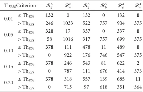
Table8: The goodness-of-fit of sum-of-exponentials model is eval-uated with two diﬀerent criteria for postnatal development of mouse cerebellum gene expression data. The first criterion com-pares with a threshold ThRSSthe ratio between the sum of squared

errors and the sum of squared measurements, for each gene. For the second criterion, the small magnitude errors are collected inRg,

and the rest of errors are included inRb. ThenRgm, 1 ≤m≤6,

is the set of all genes for which at leastmerrors belong toRg. For

eachm, the complementary set ofRm

g isRbm. The contingency

ta-bles of the gene partitions determined by the two criteria are shown for diﬀerent values of ThRSSand form∈ {4, 5, 6}.

ThRSSCriterion R6g Rb6 R5g R5b Rg4 R4b

0.01 ≤ThRSS 132 0 132 0 132 0

>ThRSS 246 1033 522 757 904 375

0.05 ≤ThRSS 320 17 337 0 337 0

>ThRSS 58 1016 317 757 699 375

0.10 ≤ThRSS 378 111 478 11 489 0

>ThRSS 0 922 176 746 547 375

0.15 ≤ThRSS 378 246 543 81 622 2

>ThRSS 0 787 111 676 414 373

0.20 ≤ThRSS 378 318 557 139 685 11

>ThRSS 0 715 97 618 351 364

errors corresponding to the analyzed gene to be small in magnitude. Since we are interested only in those genes for which the number of small magnitude errors exceeds the number of large magnitude errors, we restrict the analysis to m ∈ {4, 5, 6}, and note that the cardinalities of the selected sets are|R6

g| =378,|R5g| =654,|R4g| =1036.

We can admit with high degree of confidence that a par-ticular gene is properly selected with the criterion (11) if the gene is also included in the setR6

g. In general, choosing a par-ticular value for ThRSS leads to a partition of the genes into

two diﬀerent groups. Similarly, selecting the value ofmleads to another two-groups partition of the gene set. The contin-gency tables, shown inTable 8, are very convenient for com-paring the partitions obtained with various values of ThRSS

andm. Recall that R6

g set contains all genes for which the magnitudes of all errors are small. According to the results in

Table 8, choosing ThRSSto be 0.01 or 0.05 implies that some

genes fromR6

g are considered to have poor fit with sum-of-exponentials model. For ThRSS=0.05, 58 genes fromR6g are deemed as poor fit for sum-of-exponentials model, while 17 genes fromR6_bare assumed to fit well the model. When the decision is based on a threshold value ThRSS ≥ 0.1, all 378

genes in the setR6

g are qualified as well fitted by the model. Remark from the last column inTable 8that for ThRSS≤0.1

none of the genes with less than four errors inRgare selected by the criterion (11). These properties recommend to choose ThRSS=0.1. To illustrate the accuracy of modelling gene

ex-pressions with sum of exponentials, we plot inFigure 1the original measurements and the optimal model for two genes. Based on criterion (11) with ThRSS =0.1, we select 489

(11)

0 5 10 15 20 25 30 35 40 45

−1 5

−1

−0 5 0 0 5 1 1 5 2

Time (days)

Gene

expression

Original measurements Optimal model

0 5 10 15 20 25 30 35 40 45

−2

−1 5

−1

−0 5 0 0 5 1 1 5

Time (days)

Gene

expression

Original measurements Optimal model

Figure1: Two genes and their associated models. (a) Time series for a gene measured during postnatal development of mouse cere-bellar cortex. The gene has index 297 inhttp://physiolgenomics. physiology.org/cgi/content/full/8/2/131/DC1/2. The optimal num-ber of exponentials is p∗ ₌ _{2, the gains are [ ˆ}_α

1 αˆ2] =

[2.55 1.63], the time constants are [ ˆτ1 τˆ2] = [15.20 2.80], and

RSS(p∗₎_/6

i=1z(ti)2 = 0.010. (b) Time series of the gene having

index 1303 in the URL stated above, measured during the postna-tal development of dentate gyrus of mouse hypocampus: the esti-mated parameters arep∗ ₌_{2, [ ˆ}_α

1αˆ2]=[−5.55 16.30], [ ˆτ1τˆ2]=

[7.10 1.00], and RSS(p∗₎_/6

i=1z(ti)2=0.002.

them. We apply the same procedure for the gene expressions measured during postnatal development of mouse dentate gyrus, and the number of genes for which the model with sum of exponentials fits well is 561 out of 1412.

4.3. Clustering the selected genes

We use CEM to group intoNTC = 3 clusters the time

con-stants associated with the 489 genes selected from cerebel-lum data set. After running the algorithm from 40 diﬀerent initialization points, the resulting centroids are T1 = 1.88,

T2 =6.16,T3 =15.41. We note that the time constants are

clustered after eliminating the outliers which are the values smaller than 1, or larger than 35. Based on the method de-scribed in Section 3, we use the clusters already found for time constants to group the genes, and the resulting num-ber of gene clusters is NGC = 6. Recall that two genes are

pooled together in the same cluster when both sets of time constants are associated to the same sequence of centroids. We assign to the gene clusters labels fromC1toC6, and list

for every cluster the corresponding sequence of centroids: C1:{T1},C2:{T2},C3 :{T3},C4:{T1,T2},C5:{T1,T3},

C6:{T2,T3}. Observe that there is no gene for which the set

of time constants contains representatives from all clusters whose centroids areT1,T2,T3.

Table9: Enrichment of functions in clusters of gene expressions measured during mouse cerebellar development. For each clusterC and for each functional categoryF, the number of genesv(C,F) that belong both toCandF is given. The enrichment is marked with shades. Statistical tests are based on hypergeometric distri-bution. The following acronyms are used for the functional cate-gories: GF: growth factors and their receptors, IST: intracellular sig-nal transduction (except kinases), DEV: development, PSOM: pro-teosome, T: transcription factors, C: carbohydrate metabolism, CY: cytoskeleton, STK: serine/threonine kinase, SY: synaptic compo-nent, GR: cell growth-related, B: brain and neuron, PS: ribosomal proteins, GANN: oncogenes and their relates.

Func. categ. C1 C2 C3 C4 C5 C6 # genes

GF 4 0 1 0 0 0 11

IST 8 1 2 2 2 1 47

DEV 1 5 2 1 0 0 22

PSOM 1 4 0 1 0 0 17

T 3 7 3 0 0 0 37

C 0 3 0 2 0 0 14

CY 7 8 0 0 0 0 48

STK 0 1 3 2 0 0 19

SY 1 0 2 0 1 1 15

GR 2 2 2 0 0 0 15

B 5 15 9 8 3 1 116

PS 8 2 2 16 1 0 50

GANN 2 0 1 2 0 0 11

Total 141 143 67 105 28 5 1412

Then we focus on the time constants corresponding to the 561 genes selected from mouse dentate gyrus data set. After dropping the outliers, the time constants are grouped by CEM in three clusters whose centroids are T1 = 1.95,

T2 = 5.58, and T3 = 19.38. Remark that the centroids are

close to those determined for the cerebellum data. Moreover, the number of gene clusters is also six, and the sequence of centroids corresponding to every gene cluster is the same as for the cerebellum data.

4.4. Enrichment of functional categories

(12)

Table10: Enrichment of functions in clusters of gene expressions measured during mouse cerebellar development. Statistical tests for enrichment are based on binomial distribution. The acronyms for the functional categories are the same as inTable 9.

GF 4 0 1 0 0 0 11

IST 8 1 2 2 2 1 47

DEV 1 5 2 1 0 0 22

PSOM 1 4 0 1 0 0 17

T 3 7 3 0 0 0 37

STK 0 1 3 2 0 0 19

SY 1 0 2 0 1 1 15

GR 2 2 2 0 0 0 15

B 5 15 9 8 3 1 116

PS 8 2 2 16 1 0 50

GANN 2 0 1 2 0 0 11

Total 141 143 67 105 28 5 1412

Table11: Enrichment of functions in clusters of gene expressions measured during mouse dentate gyrus development. For each clus-terC and for each functional category F, the number of genes

v(C,F) that belong both toCandF is given. The enrichment is marked with shades. Statistical tests are based on hypergeometric distribution. The following acronyms are used for the functional categories: STK: serine/threonine kinase, TES: testis, SY: synap-tic component, CR: chromosome component, E: electron transfer, SEC: secretory pathway, B: brain and neuron, L: lipid metabolism, GANN: oncogenes and their relates, PS: ribosomal proteins, A: amino acid metabolism, CHAP: chaperonines.

STK 7 1 2 1 2 0 19

TES 5 1 0 4 0 0 16

SY 4 1 1 2 1 1 15

CR 4 1 0 1 0 0 16

E 1 6 1 3 0 0 26

SEC 2 1 2 0 0 0 10

B 16 15 13 9 2 1 116

L 1 3 3 1 0 0 19

GANN 0 2 0 3 0 0 11

PS 7 5 2 7 0 0 50

A 2 0 1 1 3 0 17

CHAP 1 1 2 0 2 0 17

Total 165 152 100 100 36 8 1412

Prob{V > v(C,F)}<0.05, where

ProbV > v(C,F)=1− v(C,F)

i=0

qM

i

(1−q)M m−i

M m

. (12)

SinceMtakes large values for microarray data, numeri-cal diﬃculties occur when computing the expression above.

Table12: Enrichment of functions in clusters of gene expressions measured during mouse dentate gyrus development. Statistical tests for enrichment are based on binomial distribution. The acronyms for the functional categories are the same as inTable 11.

STK 7 1 2 1 2 0 19

TES 5 1 0 4 0 0 16

SY 4 1 1 2 1 1 15

CR 4 1 0 1 0 0 16

E 1 6 1 3 0 0 26

B 16 15 13 9 2 1 116

SEC 2 1 2 0 0 0 10

L 1 3 3 1 0 0 19

GANN 0 2 0 3 0 0 11

PS 7 5 2 7 0 0 50

A 2 0 1 1 3 0 17

CHAP 1 1 2 0 2 0 17

Total 165 152 100 100 36 8 1412

Relying on the theoretical result [34], which claims that the limit of the hypergeometric distributionH(M,m;q) asM→ ∞is the binomial distribution Bi(m,q), the probability func-tion ofV is modelled by Bi(m,q), and (12) will be replaced by

ProbV > v(C,F)=1− v(C,F)

i=0

m

i

qi₍₁₋_q)m−i_. ₍₁₃₎

We use next both (12) and (13) to investigate the enrich-ment of functional categories in the examples from the devel-opmental biology. We report in Tables9,10,11, and12the results obtained when testing the enrichment of functional categories in clusters found as described above. The fol-lowing supplementary conditions are added to the tests in (12) and (13): to decide that the functional category F is enriched in clusterC, it is necessary that at least 10 genes on the microarray belong toF, and at least 2 genes fromC belong toF. To refer to various functions, we use in Tables

9, 10, 11, and 12 the acronyms defined at http://physiol-genomics.physiology.org/cgi/content/full/4/2/155/DC1/2.

Comparing the results in Tables9and10, we remark that almost the same functions are found to be enriched by statis-tical tests (12) and (13). Applying the binomial distribution model seems to be more restrictive in the sense that the func-tions C and CY are reported as enriched inTable 9, but not inTable 10.

(13)

The very last observation has a special importance in comparison with the results reported in [1, 3] where en-riched functions have been found only for the clusters in cerebellum data. Our clustering procedure allows to find en-riched functions for both cerebellum data and dentate gyrus data, and some of these functions are the same for the two data sets. It is widely accepted in biology that cerebellar cor-tex and the dentate gyrus have common features [3], there-fore the findings of the newly introduced algorithm can be explained based on biological knowledge. The biological sig-nificance of our results still remains to be further investigated in the future.

5. CONCLUSION

In this paper, we propose a new approach for clustering the gene expression data that are time series. The key step of the algorithm consists in fitting a sum of exponentials to the nonuniformly sampled points of every time series. The op-timal number of exponentials is inferred relying on a new information theoretic criterion which is defined based on NML estimator [28,29]. The estimation method is tested with carefully crafted data, and the results are compared with Cram´er-Rao lower bound. The conclusions drawn for simu-lated data allow to define a criterion that determines when the sum of exponentials model fits well the measured data. The clustering procedure is applied for data sets from devel-opmental biology [1,3], and the enrichment of functional categories is investigated.

APPENDICES

A. THE SEPARABILITY OF PARAMETERS FOR THE LS PROBLEM

Nonlinear LS problems are in general diﬃcult to solve, and it is of interest to reduce the problem to one of a smaller dimen-sionality if the optimization can be analytically performed over a subset of variables, for fixed values of the remaining variables. This can be readily achieved for model (2) by re-stating the LS problem as follows.

Minimizeε2_{, where}_ε_{is the error vector}_ε=_z₋_B(b)a and where b is the vector [β1,. . .,βp], a is the vec-tor [α1,. . .,αp], and B is the matrix with entries bi j = exp(−tiβj), for 1≤i≤nand 1≤j≤p. Recall that the vec-tor of measurements isz =[z(t1)· · ·z(tn)]. Assume that n≥p, which is the case of interest where the number of ex-ponentials does not exceed the number of measurements.

For a givenb, we denote by â(b) the vector that min-imizes ε2_{, which results to be the linear LS solution} â(b)=(BB)−1_B_{z, if the matrix}_B_B_{is nonsingular. The} matrixBhas all columns independent, since everyp×p mi-nor is a generalized Vandermonde matrix with nonzero de-terminant. Thus, the matrixBBis positive definite and non-singular, andâ(b)=(BB)−1_B_z_{is the unique minimizer of} ε2 _{for a given}_b_{vector. Evaluating}_ε2_{at the value}_â(b), we findε2₌_z_(I₋_B(B_B)−1_B_{)z, which is now a} nonlin-ear criterion in the reduced set of parametersb, much easier to solve when compared to the original problem having as parameters the entries of the vectorsaandb.

B. COMPUTATION OF CRAM ´ER-RAO LOWER BOUND (CRLB)

Since the samples are statistically independent, we obtain the following expression of the log-likelihood function, under the hypothesis of white Gaussian noise with zero mean and varianceσ2_:

Λz|θγ

= −n 2ln

2πσ2₋ 1

2σ2

n

i=1

zti

−yti|θγ

2

, (B.1)

wherezis the vector of measurements, and the set of param-etersθγis given in (6). In this section, we drop the indexγ, and writeθinstead ofθγ. The expression of the Fisher infor-mation matrix is

 J 0

0 n

2σ4



_. (B.2)

We focus on the entries of the blockJ:

Jm= −E

∂2_Λ_(z_|_θ₎ ∂θ∂θm

=E

∂Λ(z|θ) ∂θ

m

, (B.3)

where the derivatives are evaluated at the true value of θ, and the expectation is taken with respect to the probability density function of zconditional to the model parameters [23].θandθmare the’th and them’th entries ofθ, where 1 ≤ ,m ≤ 2p. A well-known result on CRLB for general Gaussian case [23] implies

Jm= 1 σ2

n

i=1

∂yti|θ ∂θ

m

. (B.4)

From y(ti|θ) = pj=1αjδtji, or equivalently, y(ti|θ) =

p

j=1θj(θj+p)ti, we readily obtain

∂yti|θ ∂θ =   

θ+p

ti

, 1≤≤p,

θ−pti

θ

ti−1

, p+ 1≤≤2p, (B.5)

which leads to

Jm=

                                                           1 σ2 n

i=1

θ+p

ti θm+p

ti ,

1≤,m≤p, 1

σ2

n

i=1

ti2θ−p

θ

ti−1

θm−p

θm

ti−1

,

p+ 1≤,m≤2p, 1

σ2

n

i=1

θ+p

ti θm−pti

θm

ti−1

,

1≤≤p,p+ 1≤m≤2p, 1

σ2

n

i=1

θ−pti

θ

ti−1

θm+p

ti ,

p+ 1≤≤2p, 1≤m≤p.

(14)

When the set of parameters for the signal model isθγ(7), letGbe the block of the Fisher information matrix similar to J. For simplicity, we use the notationθ instead ofθγ. Based on the result from [23] on vector parameter transformations, the relationship between the entries of the matricesGandJ is given by

Gm=Jm

∂θ ∂θ

∂θm ∂θ m

, (B.7)

where 1≤,m≤2p. For 1≤≤ p, we have∂θ/∂θ =1, while forp+ 1≤≤2p,

∂θ ∂θ

=∂δ ∂τ =exp

−T0

τ T0

τ2

=δT0 τ2

=T0 θ

θ

2. (B.8)

Based on the equations (B.6) and (B.8), we can easily calcu-late the entries of the matricesJandG, and further compute the CRLB.

ACKNOWLEDGMENTS

This work has been supported by Academy of Finland project no. 44876. The material in this manuscript was presented in part at GENSIPS 2004, Workshop on Genomic Signal Pro-cessing and Statistics, Baltimore, Maryland, USA, May 26– 27, 2004.

REFERENCES

[1] R. Matoba, S. Saito, N. Ueno, C. Maruyama, K. Matsubara, and K. Kato, “Gene expression profiling of mouse postnatal cerebellar development,” Physiol. Genomics, vol. 4, pp. 155– 164, 2000.

[2] J. Ollila and M. Vihinen, “Microarray analysis of B cell stim-ulation,”Vitam. Horm., vol. 64, pp. 77–99, 2002.

[3] S. Saito, R. Matoba, N. Ueno, K. Matsubara, and K. Kato, “Comparison of gene expression profiling during postnatal development of mouse dentate gyrus and cerebellum,” Phys-iol. Genomics, vol. 8, pp. 131–137, 2002.

[4] K. Y. Yeung, C. Fraley, A. Murua, A. E. Raftery, and W. L. Ruzzo, “Model-based clustering and data transformations for gene expression data,”Bioinformatics, vol. 17, no. 10, pp. 977– 987, 2001.

[5] A. Schliep, A. Schonhuth, and C. Steinhoﬀ, “Using hidden Markov models to analyze gene expression time course data,” Bioinformatics, vol. 19, no. 1, pp. i255–i263, 2003.

[6] M. J. L. de Hoon, S. Imoto, and S. Miyano, “Statistical anal-ysis of a small set of time-ordered gene expression data using linear splines,”Bioinformatics, vol. 18, no. 11, pp. 1477–1485, 2002.

[7] C. S. Moller-Levet, K.-H. Cho, and O. Wolkenhauer, “Mi-croarray data clustering based on temporal variation: FCV with TSD preclustering,” Applied Bioinformatics, vol. 2, no. 1, pp. 35–45, 2003.

[8] M. F. Ramoni, P. Sebastiani, and I. S. Kohane, “Cluster anal-ysis of gene expression dynamics,”Proceedings of the National Academy of Sciences of the USA, vol. 99, no. 14, pp. 9121–9126, 2002.

[9] C. S. Moller-Levet, K.-H. Cho, H. Yin, and O. Wolken-hauer, “Clustering of gene expression time series data,” Tech. Rep., Systems Biology and Bioinformatics Group, Univer-sity of Rostock, Germany, November 2003, http://www.sbi. uni-rostock.de/publications.htm.

[10] I. T˘abus¸ and J. Astola, “Clustering the non-uniformly sam-pled time series of gene expression data,” inProc. Seventh EURASIP-IEEE International Symposium on Signal Process-ing and Its Applications (ISSPA ’03), vol. 2, pp. 61–64, Paris, France, July 2003.

[11] C. D. Giurc˘aneanu, I. T˘abus¸, and J. Astola, “Clustering time series gene expression data based on sum-of-exponentials fit-ting,” inWorkshop on Genomic Signal Processing and Statistics (GENSIPS ’04), Baltimore, Md, USA, May 2004, CD-ROM (4 pages).

[12] T. Chen, H. L. He, and G. M. Church, “Modeling gene ex-pression with diﬀerential equations,” inBiocomputing 1999: Pacific Symposium on Biocomputing, R. Altman, A. Dunker, L. Hunter, T. Klein, and K. Lauderdale, Eds., vol. 4, pp. 29–40, World Scientific Publishing, Mauna Lani, Hawaii, USA, Jan-uary 1999.

[13] M. de Hoon, S. Imoto, K. Kobayashi, N. Ogasawara, and S. Miyano, “Inferring gene regulatory networks from time-ordered gene expression data of Bacillus Subtilis using diﬀer-ential equations,” inBiocomputing 2003: Proc. Pacific Sympo-sium, R. B. Altman, A. K. Dunker, L. Hunter, T. A. Jung, and T. E. Klein, Eds., vol. 8, pp. 17–28, World Scientific Publishing, Kauai, Hawaii, USA, January 2003.

[14] C. D. Giurc˘aneanu, I. T˘abus¸, and J. Astola, “Linear algebra re-sults applied to diﬀerential equations model for gene expres-sion data,” inThe 2nd TICSP Workshop on Computational Sys-tems Biology (WCSB ’04), pp. 31–32, Helsinki-St.Petersburg, June 2004.

[15] I. T˘abus¸, C. D. Giurc˘aneanu, and J. Astola, “Genetic net-works inferred from time series of gene expression data,” in Proc. First International Symposium on Control, Communica-tions and Signal Processing (ISCCSP ’04), pp. 755–758, Ham-mamet, Tunisia, March 2004.

[16] M. R. Osborne and K. Smyth, “A modified Prony algorithm for fitting functions defined by diﬀerence equations,” SIAM Journal of Scientific and Statistical Computing, vol. 12, no. 2, pp. 362–382, 1991.

[17] H. Ouibrahim, “Prony, Pisarenko, and the matrix pencil: a unified presentation,”IEEE Trans. Acoust., Speech, Signal Pro-cessing, vol. 37, no. 1, pp. 133–134, 1989.

[18] D. Kundu and A. Mitra, “Fitting a sum of exponentials to equispaced data,” Sankhya, Series B, vol. 60, no. 3, pp. 448– 463, 1998.

[19] K. Holmstrom and J. Petersson, “A review of the parame-ter estimation problem of fitting positive exponential sums to empirical data,” Applied Mathematics and Computation, vol. 126, no. 1, pp. 31–61, 2002.

[20] M. Al-Baali and R. Fletcher, “An eﬃcient line search for non-linear least squares,” Journal of Optimization Theory and Ap-plications, vol. 48, no. 3, pp. 359–377, 1986.

[21] J. Petersson and K. Holmstrom, “Initial values for the expo-nential sum least squares fitting problem,” Tech. Rep. IMa-TOM-1998-01, Department of Mathematics and physics, M¨alardalen University, Sweden, http://www.mdh.se/ima/ personal/khm01/tom/tom-prints/print-technical reports. htm, June 1998.

[22] A. R. Gallant,Nonlinear Statistical Models, John Wiley & Sons, New York, NY, USA, 1987.

[23] S. M. Kay, Fundamentals of Statistical Signal Processing, Vol-ume I: Estimation Theory, Prentice-Hall, Englewood Cliﬀs, NJ, USA, 1993.

[24] P. Stoica and R. L. Moses, Introduction to Spectral Analysis, Prentice-Hall, Englewood Cliﬀs, NJ, USA, 1997.