R E S E A R C H
Open Access
Non-unitary matrix joint diagonalization for
complex independent vector analysis
Hao Shen and Martin Kleinsteuber
*Abstract
Independent vector analysis (IVA) is a special form of independent component analysis (ICA), which has demonstrated its prominent performance in solving convolutive blind source separation (BSS) problems in the frequency domain. Most IVA algorithms are based on optimizing certain contrast functions, where the main difficulty of these approaches lies in finding a reliable and fast estimation of the unknown distribution of sources. Despite the rich availability of efficient tensorial approaches to the standard ICA problem, these methods have not been explored considerably for IVA. In this article, we propose a matrix joint diagonalization approach to solve the complex IVA problem. The new factorization neither relies on a whitening process, nor does it require an estimate of the joint probability distribution of the dependent signal groups. The latter is in contrast to most IVA approaches up to date. The underlying geometry of the problem is investigated together with a critical point analysis of the resulting cost function. A conjugate gradient algorithm on the appropriate manifold setting is developed.
1 Introduction
Independent component analysis (ICA) is a standard sta-tistical tool for solving the blind source separation (BSS) problem. BSS aims to recover source signals from the observed mixtures, without knowing either the distribu-tion of the sources or the mixing process. Applicadistribu-tion of the standard ICA model is often limited, since it requires mutual statistical independence between all individual components. However, in many applications, there exist groups of signals of interest, where components from different groups are mutually statistically independent
indeed, but wheremutual statistical dependenceoccurs between components in the same group. Such problems can be tackled by a technique now referred to as multidi-mensional independent component analysis (MICA) [1], or independent subspace analysis (ISA) [2].
A special form of ISA arises in solving the BSS prob-lem with convolutive mixtures [3]. After transferring the convolutive observations into the frequency domain via short-time Fourier transforms, the convolutive BSS prob-lem results in a collection of instantaneous complex BSS problems in each frequency bin. After solving the sub-problems individually, the final stage faces the challenge
*Correspondence: [email protected]
The Department of Electrical Engineering and Information Technology, Technische Universit¨at M ¨unchen, M ¨unchen, Germany
of aligning all statistically dependent components from different groups, which is referred to as thepermutation
problem. To avoid this problem, a new approach named
independent vector analysis (IVA) has been proposed in [4]. Besides its application in convolutive BSS problem, IVA has also recently been applied to analyze multivari-ate Gaussian models, cf. [5,6]. In the current literature, the majority of IVA algorithms are based on optimizing certain contrast functions, cf. [5,7-9]. The main difficulty of these contrast function based approaches lies in esti-mating the unknown distribution of the sources, which usually requires a large number of observations [10].
On the other hand, tensorial approaches are efficient and richly available to solve both the ICA and ISA prob-lems. In particular, joint block diagonalization approaches are shown to be effective methods for solving the ISA problem, cf. [11,12], and are inherently applicable to IVA. However, such general joint block diagonalization approaches do not take the intrinsic structure of the IVA problem into account. Recent study in [13] proposes a joint diagonalization approach of cross cumulant matri-ces to solve the complex IVA problem. More recently, the present authors have developed a similar approach of jointly diagonalizing both cross covariance and cross pseudo covariance matrices, cf. [14]. In this article, we extend the previous study in [14], and adapt the so-called complex oblique projective (COP) manifold, which
has proven to be an appropriate setting for the stan-dard instantaneous complex ICA problem [15], to the current scenario. Finally, an efficient conjugate gradient (CG) based IVA algorithm is proposed, and numerical experiments are provided to demonstrate the convergence properties of the proposed CG algorithm, and to com-pare its performance with two recently developed IVA algorithms in terms of separation quality.
2 Notations
Throughout the article,(·)denotes the matrix transpose, (·)H the Hermitian transpose,(·)the entry-wise complex conjugate of a matrix, and byGl(m)the set of allm×m
invertible complex matrices. The Frobenius norm of a matrixA∈Cm×nis denoted byAF:=tr(AAH), where tr(·)is the trace of a square matrix. Given a square matrix
Z∈Cm×m, ddiag(Z)forms a diagonal matrix whose diag-onal entries are those ofZ, and off(Z)generates a matrix by setting all diagonal entries ofZ to zero, i.e. off(Z) :=
Z−ddiag(Z).
In this study, we consider an m-dimensional complex signals(t)=[s1(t),. . .,sm(t)]∈Cmas anm-dimensional
complex stochastic process indexed by the variablet. The empirical expectation of a random variable sis denoted byE[s(t)]= T1Tt=1s(t), whereT is the number of sam-ples. As usual for the standard ICA model, we assume without loss of generality thatE[s(t)]=0. The empirical covariance and pseudo-covariance matrix of complex sig-nals s(t)are referred to as cov(s(t)) := E[s(t)s(t)H] and pcov(s(t)):=E[s(t)s(t)], respectively.
3 Problem description
It is known that convolutive BSS problems can be trans-formed into in the frequency domain, and can be solved as instantaneous complex BSS problems for every frequency simultaneously, when the demixing filter is sufficiently longer than the mixing filter, cf. [16,17]. In this study, we consider the spectral time-frequency representation of a signal in terms of a short-time Fourier transformation that is centered at time t. Letwi(t,f) ∈ Cand si(t,f) ∈ C
denote the coefficient of the center frequencyf of theith observationwi(t) and theith source signal si(t),
respec-tively. Then, for a given pair(t,f), the Fourier coefficients of the observations and the sources obey the equality
w(t,f)=Afs(t,f), (1)
wherew(t,f) :=[w1(t,f),. . .,wm(t,f)]∈ Cm, s(t,f) :=
[s1(t,f),. . .,sm(t,f)]∈ Cm, andAf ∈ Cm×mserves as a
complex mixing matrix. More compactly, for a fixed fre-quencyf, we get a standard instantaneous complex BSS problem as
W(f)=AfS(f), (2)
where W(f) ∈[w(1,f),. . .,w(T,f)]∈ Cm×T andS(f) ∈ [s(1,f),. . .,s(T,f)]∈Cm×T, withT being the number of chosen time frames. One popular approach to solve the convolutive BSS problem is to solve the individual instan-taneous BSS problem at each frequency (2), and then assemble the results from each frequency to reconstruct the estimated signal in the time domain [18].
Let us denote the rows of S(f) by si(f) =
[si(1,f),. . .,si(T,f)]∈ C1×T fori = 1,. . .,m. Following
the assumption of statistical independence between the sources, the complex valued signals si(f) and sj(f) are statistically independentfori=j. In contrast, we assume that for a pair of frequencies (fp,fq) with fp = fq, the
complex signalssi(fp)andsi(fq)arestatistically dependent
for a given source. The development of IVA is inspired by this cross frequency structure. It aims to find a set of demixing matrices{Xf} ⊂Gl(m)via
Y(f)=XfHW(f), (3)
such that
(1) all sub-ICA problems are solved, and
(2) the statistical alignment between groups is restored, i.e. the estimatedi th signals{yi(f)}are mutually statistically dependent.
The main idea for our approach is to exploit the cross covariance matrices between groups of observations defined as
cov(W(fi),W(fj)):=
1
T T
t=1
w(t,fi)w(t,fj)H
=A(fi)
1
T T
t=1
s(t,fi)s(t,fj)H
=:cov(S(fi),S(fj))
A(fj)H.
(4)
Similarly, the so-calledpseudo cross covariance, defined as
pcov(W(fi),W(fj)):=
1
T T
t=1
w(t,fi)w(t,fj)
=A(fi)pcov(S(fi),S(fj))A(fj),
(5)
also allows to gain additional information about the second-order statistics of the involved signals. In this study, we assume that cross covariances between sources in all groups do not vanish. The assumption of statistical independence between the source signals implies that the cross covariance matrix cov(S(fi),S(fj)) and the pseudo
cross covariance matrix pcov(S(fi),S(fj))are diagonal for
cross covariance and pseudo cross covariance matrices at different time instances.
To summarize, we are interested in solving the following problem. For a complex IVA problem with k subprob-lems, we consider the cross covariance and pseudo cross covariance matrices atntime instances, i.e. for alli,j =
1,. . .,k andt = 1,. . .,n, a set of matrices{Cij(t)}i<j and
a set of complex symmetric matrices{R(ijt)}i<j, which are
constructed by
Cij(t)=Ai(ijt)A H
j and R
(t)
ij =Ai(ijt)Aj, (6)
where(ijt),(ijt) ∈Cm×mare diagonal. The task is to find a set of matrices{Xi}ki=1⊂Gl(m)such that
XiHC(ijt)Xj and XiHR
(t)
ij Xj, (7)
for all i < j and t = 1,. . .,n, are simultaneously, or approximately simultaneously diagonalized. In this study, we study the noise free IVA problem as defined in (2), and neglect the cross covariance matrix estimation errors due to the finite sample size effect. In other words, we assume that both sets ofCij(t)’s andR(ijt)’s are jointly diagonalizable. Note that the above problem is similar to the simul-taneous SVD formulation proposed in [20], where only the situation with two transform matrices is studied, i.e.
k= 2. To the contrary, our current setting deals with the cases of multiple transform matrices{Xi}i=1,...,k, which are
not restricted to be unitary. Finally, instead of consider-ing second order cross covariance matrices, our developed approach can be generalized to the high order cross cumu-lants. We refer to [17] for further details.
4 Diagonality measure and the COP manifold
Our cost function to tackle problem (7) originates from the popular off-norm function that measures the squared Frobenius norm of the off-diagonal entries of the involved matrices. We develop an appropriate mathematical setting on the subsequently defined complex oblique projective
(COP) manifold to provide its critical point analysis.
4.1 Derivation of the cost function
For legibility reasons, from now on, we only consider the problem of simultaneously diagonalizing the covariance matrices, i.e. the first condition in (7). The combina-tion with the addicombina-tional requirement that also the pseudo cross covariance matrices may be used for estimating the demixing matrix is straightforwardly adapted to our setting and not further discussed here.
Let us define the off-norm function as
g:(Gl(m))k →R,
g(X1,. . .,Xk):= k
i<j n
t=1 1 2off(X
H iC
(t)
ij Xj)
2
F.
(8)
Due to the noise-free assumption and since we neglect finite sample size effects, the set of joint diagonalizers (X1∗,. . .,Xk∗) of theCij(t) in Equation (7) is a global min-imum of g, that is g(X1∗,. . .,Xk∗) = 0. It is clear that a minimization approach without further constraints on the Xi would drive all diagonalizers to zero. In order to
avoid such trivial solutions and to regularize the mini-mization problem, the authors in [21] propose to restrict all columns of transform matrices to have unit norm. This set is known as the oblique manifold, which has been shown to be an appropriate setting for matrix diagonal-ization, cf. [22]. Its complex counterpart is the so-called
complex oblique manifold
Ob(m):=X∈Gl(m)ddiag(XHX)=Im
(9)
and we denote by Obk(m) the product manifold of k
copies of Ob(m). The restriction of the off-norm cost function (8) is denoted by
g1:Obk(m)→R,
g1(X1,. . .,Xk):= k
i<j n t=1 1 2
off(XiHCij(t)Xj)
2
F.
(10)
Now denote thepth column ofXi byxip. It is obvious
that the functiong1is invariant with respect to the phase
difference of each column xip, which reflects the
well-known scaling ambiguity of complex ICA problems. By a further calculation,g1has the form
g1(X1,. . .,Xk)=
1 2
k
i<j n t=1 m p=q
xHipCij(t)xjq 2
= 1
2
k
i<j n t=1 m p=q
xHipC(ijt)xjq
xHipCij(t)xjq
H
= 12
k
i<j n t=1 m p=q
trxipxHip
C(ijt)xjqxHjq
Cij(t)H.
(11)
Instead of fixing a phase for eachxip, in this study we
employ an elegant mathematical setting for the problem. Recall the fact that eachxipxHip defines a Hermitian
rank-one projector, the set of which identifies the (m − 1) -dimensionalcomplex projective spaceCPm−1, i.e.
CPm−1=P∈Cm×mPH=P,P2=P, tr(P)=1.
(12)
invertibility ofXi), we naturally arrive at the following set,
which we refer to as thecomplex oblique projective (COP) manifold,
Q(m):=
(P1,. . .,Pm)Pi∈CPm−1, det
m
i=1 Pi
>0
.
(13)
The off-norm cost functiong1now induces the
follow-ing functiong2 on the COP manifold. Namely, ifQk(m)
denotes thek-times product ofQ(m),g2is given by
g2:Qk(m)→R,
g2(P1,. . .,Pk):= k
i<j n
t=1
m
p=q
trPipCij(t)PjqCij(t)H,
(14)
withPi:=(Pi1,. . .,Pim).
4.2 The geometry of the complex oblique projective manifold
In this section, we recall some basic facts and con-cepts that are necessary for developing a Riemannian CG algorithm on the COP manifold, cf. [23]. In particular, we require a formula for the parallel transport and the geodesics of the COP manifold. We endowQ(m)with the standard Riemannian metric
(A1,. . .,Am),(B1,. . .,Bm):=
i
tr(AiBi), (15)
inherited from the Euclidean metric of them-fold product of Hermitian matrices. With this,Q(m) is an open and dense Riemannian submanifold of them-times product of CPm−1with the standard metric, i.e.
Q(m)=:CPm−1m, (16)
where Q(m) denotes the closure of Q(m). Accordingly, the tangent spaces, the geodesics, and the parallel trans-port forQ(m)and(CPm−1)mcoincide locally and thus are easily derived from the geometry ofCPm−1. We refer to [24] for further discussions and details aboutCPm−1.
Let us denote by
u(m):=∈Cm×m= −H
(17)
the set of skew-Hermitian matrices. The tangent space at
PinCPm−1is given by
TPCPm−1= {[P,]|∈u(m)} (18)
where [A,B] :=AB−BAis the matrix commutator. Then, the tangent space atP = (P1,. . .,Pm) ∈ Q(m)is simply
the Cartesian product
TPQ(m)∼=TP1CPm−
1×. . .×T
PmCPm−1. (19)
With the above metric, the geodesics through P ∈
CPm−1in directionZ∈T
PCPm−1are given by
γP,Z:R→CPm−1, γP,Z(t):=et[Z,P]Pe−t[Z,P],
(20)
where e(·) denotes the matrix exponential. Thus, the (locala) geodesic throughP ∈ Q(m) in direction Z := (Z1,. . .,Zm)∈TPQ(m)is given by
γP,Z(t)=
γP1,Z1(t),. . .,γPm,Zm(t)
. (21)
The parallel transport of:=(1,. . .,m)∈TPQ(m) with respect to the Levi-Civita connection along the geodesicγP,Z(t)is
τP,Z():=
τP1,Z1(1),. . .,τPm,Zm(m)
, (22)
with τP,Z being the parallel transport of ∈ TPCPm−1
with respect to the Levi-Civita connection along the geodesicγP,Z(t), i.e.
τP,Z()=e[Z,P]e−[Z,P]. (23)
ThenaturalorRiemanniangradient of a function that is the restriction of some globally defined function to a sub-manifold is simply the orthogonal projection of the Euclidean gradient onto the corresponding tangent space. For the complex projective space, this projection is given by
P:Cm×m→TPCPm−1, A→[P, [P,12(A+AH)] ] .
(24)
It is easily seen that the operator P is an
orthogo-nal projector on the tangent space TpCPm−1, i.e. that
P ◦ P(A) = P(A) and that the null space of P
is orthogonal to its image. Here, ◦ denotes the compo-sition of functions. The formulas for the tangent spaces, the geodesics, the parallel transport, and the projection onto the tangent spaces ofQk(m)follow directly from the product manifold structure.
5 Critical point analysis of the cost function
In this section, we conduct a critical point analysis of the cost function g2 on the product COP manifold. We
show that the joint diagonalizers are a non-degenerate global minimum ofg2, This is an important fact, since in
many cases the speed of convergence relies on the non-degeneracy of the minima. First of all, we present a lemma which originates from the derivation of the cost from the off-norm function.
Lemma 1.Let us assume that all Cij(t)’s are jointly diag-onalizable. If(X∗1,. . .,Xk∗) ∈ Obk(m)minimizes the cost function g1, as defined in (10), i.e. X∗iHC
(t)
ij Xj∗ = D
(t)
ij =
pro-jectorsP∗ = (P∗1,. . .,P∗k) ∈Qk(m)with P∗ip := x∗ipx∗ipH ∈
CPm−1minimizes the cost function g
2, defined in (14) and ⎧
⎨ ⎩
P∗ipCij(t)Pjq∗ =0, for p=q,
Pip∗Cij(t)Pjq∗ =dijp(t)P∗ip, for p=q. (25)
The above lemma follows directly from the condition ofXi∗HCij(t)Xj∗being diagonal, i.e. its(p,q)th entry is com-puted as
xHipCij(t)xiq=
0, forp=q,
d(ijpt), forp=q. (26)
Now, let P := (P1,. . .,Pm) ∈ Qk(m) be arbitrary.
We compute the first derivative ofg2 at P ∈ Qk(m) in
directionZ:=(Z1,. . .,Zk)∈TPQk(m)as
Dg2(P)Z=
k
i<j m
p=q n
t=1
trZipC(ijt)PjqCij(t)H
+trPipCij(t)ZjqCij(t)H.
(27)
By recalling the structure of the tangent space ofQk(m) and the result in Lemma 1, it is trivial to see that the first derivative ofg2vanishes atP∗, which corresponds to the
correct joint diagonalizers.
The remainder of this section addresses the character-ization of the Hessian ofg2at the joint diagonalizers. To
that end, we denote byoff(m) := {Z ∈ Cm×m |zii = 0, i=1,. . .,m}the set of matrices with zero diagonal. Letπ be the natural projection
π:Ob(m)→Q(m), π(X)=(x1xH1,. . .,xmxHm) (28)
and letμXbe defined as
μX:off(m)→Ob(m),
Z→X(Im+Z)diag
1
X(e1+z1),. . ., 1
X(em+zm)
,
(29)
whereejdenotes thejth standard basis vector. Note, that
μX defines a locally injective but not bijective mapping.
The composition ofπandμX, however, yields a local
dif-feomorphism. With the shorthand notationP := π(X), the mapping
φP:off(m)→Q(m), Z→π◦μX(Z) (30)
is a local parametrization around P and thus permits a local parameterization ofQk(m)via
P:offk(m)→Qk(m),
(Z1,. . .,Zk)→(φP1(Z1),. . .,φPk(Zk)),
(31)
with P(0)= P := (P1,. . .,Pk). The associated tangent
mapT P is given as
T P:Toffk(m)∼=offk(m)→TPQk(m),
(1,. . .,k)→
x11ξ(x11)θ11H +θ11ξ(x11)xH11,. . .,
xkmξ(xkm)θkmH +θkmξ(xkm)xHkm
,
(32)
whereξ(xip) := Im−xipxHipis the orthogonal projection
operator onto the complement space of xip. Let Z := T P∗()∈TP∗Qk(m). Then, we can compute the Hes-sian ofg2at the critical pointsP∗ ∈ Qk(m), i.e. the
sym-metric bilinear formHg2(P∗): TP∗Qk(m)×TP∗Qk(m)→
Rvia
Hg2(P∗)(Z,Z)=Hg2(P∗)(T P∗(),T P∗())
= d2
dt2(g2◦ P∗)(t)
t=0
= k
i<j m
p=q n
t=1
2 trZip∗C(ijt)Z∗jqCij(t)H
= k
i<j m
p=q n
t=1
2d(ijpt)θpq(i)+dijq(t)θqp(j)
2
.
(33)
The last equality holds by following the results in Lemma 1, i.e. Xi∗HC(ijt)Xj∗ = D(ijt), which is equivalent to
C(ijt) = Xi∗−HDij(t)Xj∗−1 and the fact that Z∗ip = (Im − Pi1)Xi∗θip. It can easily been seen that the Hessian form
(33) is positive definiteif and only if all(2×2)-matrices
n
t=1 ⎡ ⎣|d
(t)
ijp|2 d
(t)
ijqd
(t)
ijp
d(ijpt)dijq(t) |dijq(t)|2 ⎤
⎦ (34)
are positive definite. Since this is a generic assumption on the data, we have the following result.
Theorem 1.Generically, the global minimizer of the cost function g2is non-degenerate.
6 A CG IVA algorithm
1 3 5 7 9 11 13 10−9
10−8 10−7 10−6 10−5 10−4 10−3 10−2 10−1 100
Sweep (i)
|| P
i
− P
* ||
Figure 1Convergence behavior of the proposed CG algorithm.
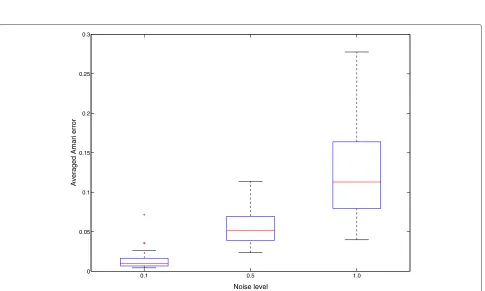
0.1 0.5 1.0
0 0.05 0.1 0.15 0.2 0.25 0.3
Noise level
Averaged Amari error
the previous sections. For an in-depth introduction on optimization on matrix manifolds, we refer the interested reader to [23].
LetMbe a submanifold of some Euclidean space with inner product ·,· and letf: M → Rbe smooth. The CG method is initialized by somex0∈Mand the descent
directionH0:= −gradf(x0)given by the Riemannian
gra-dient. Iff is the restriction of a globally defined function
f to M, the Riemannian gradient is just the orthogonal projection of the gradient off to the tangent space, i.e.
gradf(x)=x
∇f(x)
, (35)
where ∇f(x) denotes the Euclidean gradient off, and xis the orthogonal projection ontoTxM. Subsequently,
sweeps are iterated that consist of two steps, aline search
in a given direction (i.e. along a geodesic in that direc-tion) followed by an update of thesearch direction. Several different possibilities for these steps lead to different CG methods. Assume now thatxi,Hi, andGi := gradf(xi)
are given.
Given a geodesicγi with γi(0) = xi andγ˙i(0) = Hi,
the line search aims to findλi ∈ Rthat minimizes f ◦
γ: t → R. A generic approach for the step-size selec-tion is a Riemannian adapselec-tion to the backtracking line search and several modifications, cf. [23,25]. Here, we present a closed form solution for the step-size selection that works particularly well for our problem due to the quadratic nature of our cost function, cf. [26]. It is based on the assumption that a one-dimensional Newton step alongf ◦γ yields a good approximation for its minimizer. Explicitly, we choose the step-size as
λi:= −
d
dλ(f◦γ)(λ)|λ=0 d2
dλ2(f◦γ)(λ)|λ=0
. (36)
The absolute value in the denominator is chosen for the following reason. While being an unaltered one-dimensional Newton step in a neighborhood of a mini-mum the step size is the negative of a regular Newton step ifddt22(f◦γ )(λ)λ=0<0 and thus yields non-attractiveness for critical points that are not minima.
In order to compute the new search directionHi+1 ∈ Txi+1M, we need to transportHiandGi, which are tangent
toxi, to the tangent spaceTxi+1M. This is done via parallel
transport along the geodesicγ, which we denote by
τ:TxiM→Txi+1M. (37)
The updated search direction is now chosen accord-ing to a Riemannian adaption of the Hestenes-Stiefel, the Polak-Ribi`ere, or the Fletcher-Reeves update. Here, we choose a different formulation that performs slightly bet-ter in our situation than the afore mentioned ones, namely
γi:= −
Gi+1,Gi+1−τGi Hi,Gi
. (38)
Albeit the nice performance in applications, conver-gence analysis of CG methods on smooth manifolds is still an open problem. Partial convergence results for CG-methods on manifolds can be found in [27,28] and a recent result in [29].
As it is clear from the above, the first step towards for-mulating a CG algorithm for minimizing the cost function
g2is to compute its Riemannian gradient. Let us denote
by g2 the continuation of g2 to the embedding space
Cm×m×m×k. Following the computation in Equation (27),
we have the Euclidean gradient ofg2atP ∈ Qk(m), i.e.
∇g2(P):=(J1,. . .,Jk), for each elementJip∈Cm×m, as
Jip= k
j>i m p=q n t=1
C(ijt)PiqCij(t)H+ k
j<i m p=q n t=1
Cij(t)HPiqCij(t).
(39)
By projecting it onto the tangent spaceTPQk(m), we
get the Riemannian gradient of g2 at P ∈ Qk(m), i.e.
gradg2(P) := (G1,. . .,Gk) ∈ TPQk(m), for each ele-mentGip∈TPipCPm−1, as
Gip=
Pip,
Pip, k
j>i m p=q n t=1
C(ijt)PiqCij(t)H
+ k
j<i m p=q n t=1
Cij(t)HPiqCij(t)
.
(40)
The above formula for the Riemannian gradient now allows to implement the geometric CG algorithm for minimizing the functiong2as define in (14) in a
straight-forward way. A pseudo code is provided in Algorithm 1.
Algorithm 1 A CG IVA algorithm.
Input:A set of matrices{C(ijt)} ⊂Cm×mfor i,j=1,. . .,n;
Step 1:Generate an initial guess P(0)=[P(0)
1 . . .,P
(0)
k ]∈Qk(m)and seti=1;
Step 2:Compute
G(1)=H(1)=[H
1,. . .,Hk]← −gradg2(P(0))using
Equation (40);
Step 3:Seti=i+1;
Step 4:UpdatePi+1←γ
P1,H1(λi),. . .,γPk,Hk(λi)
, whereλiis computed (36);
Step 5:UpdateH(i+1)← −G(i+1)+γ
iτP(i),Hi(λi), where
G(i+1)=
gradg2(P(i)),
andγiis chosen according to Equation (38);
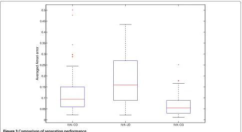
IVA−CO IVA−JD IVA−CG 0
0.05 0.1 0.15 0.2 0.25 0.3 0.35 0.4 0.45 0.5
Averaged Amari error
Figure 3Comparison of separation performance.
Step 7:IfG(i+1)is small enough, stop. Otherwise, go to Step 3;
7 Numerical experiments
In our experiment, we investigate the performance of our method in terms of both local convergence property and accuracy of estimating the joint diagonalizers.
7.1 Experiment one
The First task of our experiment is to jointly diagonalize two sets of complex matrices,{Cij(t)}i<jand{R(ijt)}i<j, which
are constructed by
Cij(t)=Aiij(t)AHj +εNijH and R
(t)
ij =Ai
(t)
ij Aj +εNijS
(41)
where the matricesAi∈Gl(m)are randomly picked, both
real and imaginary parts of the diagonal entries of(ijt)and
(ijt)are drawn from a uniform distribution on the inter-val (0, 10), the matricesNijH ∈ Cm×m andNijS ∈ Cm×m
are a Hermitian and a complex symmetric matrix, respec-tively, whose real and imaginary parts are generated from a uniform distribution on the unit interval(−0.5, 0.5), rep-resenting additive stationary noise, andε∈Ris the noise level.
In our experiments, we setm = 3,k = 3,n = 3. First of all, we choose the noise levelε = 0. A typical local convergence curve of our proposed algorithm is shown in
Figure 1. A tendency of superlinear convergence can be observed.
In order to investigate the performance of the proposed algorithm in terms of estimation accuracy, we restrictε∈
{0.1, 0.5, 1.0}, and run 50 tests. The performance index is chosen to be the averaged Amari error, proposed in [30]. Generally, the smaller the Amari error, the better the sep-aration. The quartile based boxplot of averaged Amari errors of our proposed algorithm against three different noise levels are drawn in Figure 2. Our CG algorithm demonstrates its correspondingly delaying performance with the increasing noise levels.
7.2 Experiment two
In this experiment, we compare our CG based IVA approach, referred to asIVA-CG, with two second-order statistics based IVA algorithms. We refer to one contrast optimization based IVA algorithm as IVA-CO, cf. [5,6], and the other matrix joint diagonalization based approach as IVA-JD, cf. [13]. The task of this experiment is to separate two groups of complex valued signals. We take three real audio source signals with 480,000 samples, and apply the short time Fourier transform to the sources with the number of FFT points being 1,024. By doing so, we end up with a complex IVA problem with 513 groups of statistically dependent complex signals.
this issue by only taking two neighboring frequency bins randomly at one time. The sources from each fre-quency bin are mixed independently via multiplying a mixing matrix, whose entries are drawn from a normal distribution. We run the experiment 100 times, and plot the boxplot of averaged Amari errors of the three stud-ied algorithms in Figure 3. It depicts clearly that our proposed IVA-CG algorithm outperforms the other two consistently.
8 Conclusion
We propose a matrix joint diagonalization approach to solve the complex IVA problem which does not rely on a pre-whitening step nor on the estimation of the unknown distribution of the sources. A mathematical setting is derived that allows a formulation without ambiguity on the set of unknown parameters, i.e. the dimension of the search space is maximally reduced. This leads in a natural way to a smooth manifold structure that we callcomplex oblique projective manifold, due to its close relation to the oblique manifold which consists of invertible matri-ces with normalized columns. We propose to solve the complex IVA problem via minimizing a cost function that is based on the well-known off-norm function for mea-suring joint diagonality. We show that our setting leads to a non-degenerate Hessian for the solution of the IVA problem. This is an important result for the design of minimization methods, since in many cases, the speed of convergence relies on the non-degeneracy of the min-ima. We develop a geometric CG method for solving the IVA problem and conclude by providing some numerical experiments.
Endnote
aNote, thatQ(m)is not a geodesically complete manifold.
Competing interests
The authors declare that they have no competing interests.
Acknowledgements
This study had been supported by the Cluster of Excellence
CoTeSys—Cognition for Technical Systems, funded by the Deutsche Forschungsgemeinschaft (DFG).
Received: 21 May 2012 Accepted: 31 October 2012 Published: 21 November 2012
References
1. JF Cardoso, inProceedings of the 23rdIEEE International Conference on Acoustics, Speech, and Signal Processing (ICASSP), vol. 4. Multidimensional independent component analysis, (Seattle, WA, USA, 1998) pp. 1941–1944 2. A Hyv¨arinen, PO Hoyer, Emergence of phase and shift invariant features
by decomposition of natural images into independent feature subspaces, Neural Comput.12(7), 1705–1720 (2000)
3. S Araki, R Mukai, S Makino, T Nishikawa, H Saruwatari, The fundamental limitation of frequency domain blind source separation for convolutive mixtures of speech, IEEE Trans. Speech Audio Process.11(2), 109–116 (2003)
4. I Lee, T Kim, TW Lee, inBlind Speech Separation, Signals and Communication Technology, ed. by S Makino, TW Lee, and H Sawada.
Independent vector analysis for convolutive blind speech separation, (Springer, Netherlands, 2007) pp. 169–192
5. M Anderson, XL Li, T Adalı, Complex-valued independent vector analysis: application to multivariate Gaussian model, Signal Process.
92(8), 1821–1831 (2012)
6. M Anderson, T Adalı, XL Li, Joint blind source separation with multivariate Gaussian model: algorithms and performance analysis, IEEE Trans. Signal Process.60(4), 1672–1683 (2012)
7. T Kim, Real-time independent vector analysis for convolutive blind source separation, IEEE Trans. Circ. Syst. I: Regular Papers.57(7), 1431–1438 (2010)
8. J Hao, I Lee, TW Lee, TJ Sejnowski, Independent vector analysis for source separation using a mixture of Gaussians prior, Neural Comput. 22(6), 1646–1673 (2010)
9. I Lee, GJ Jang, Independent vector analysis based on overlapped cliques of variable width for frequency-domain blind signal separation, EURASIP J. Adv. Signal Process.113, 1–12 (2012)
10. S Bermejo, Finite sample effects in higher order statistics contrast functions for sequential blind source separation, IEEE Signal Process. Lett. 12(6), 481–484 (2005)
11. H Ghennioui, EM Fadaili, N Thirion-Moreau, A Adib, E Moreau, A nonunitary joint block diagonalization algorithm for blind separation of convolutive mixtures of sources, IEEE Signal Process. Lett.
14(11), 860–863 (2007)
12. H Ghennioui, N Thirion-Moreau, E Moreau, D Aboutajdine, Gradient-based joint block diagonalization algorithms: application to blind separation of FIR convolutive mixtures, Signal Process.90(6), 1836–1849 (2010) 13. XL Li, T Adalı, M Anderson, Joint blind source separation by generalized
joint diagonalization of cumulant matrices, Signal Process.91(10), 2314–2322 (2011)
14. H Shen, M Kleinsteuber, inProceedings of the 10thInternational Conference on Latent Variable Analysis and Signal Separation (LVA/ICA), vol. 7191 Lecture Notes in Computer Science, ed. by F Theis, A Cichocki, A Yeredor, and M Zibulevsky. A matrix joint diagonalization approach for complex independent vector analysis, (Springer-Verlag, Berlin/Heidelberg, 2012) pp. 66–73
15. H Shen, M Kleinsteuber, inLecture Notes in Computer Science, Proceedings of the 9thInternational Conference on Latent Variable Analysis and Signal Separation, vol. 6365. Complex blind source separation via simultaneous strong uncorrelating transform, (Springer-Verlag, Berlin/Heidelberg, 2010) pp. 287–294
16. P Smaragdis, Blind separation of convolved mixtures in the frequency domain, Neurocomputing.22, 21–34 (1998)
17. P Comon, C Jutten,Handbook of Blind Source Separation: Independent Component Analysis and Applications. (Academic Press Inc, San Diego, USA, 2010)
18. S Makino, TW Lee, H Sawada,Blind Speech Separation Signals and Communication Technology. (Springer, Netherlands, 2007)
19. S Hosseini, Y Deville, H Saylani, Blind separation of linear instantaneous mixtures of non-stationarysignals in the frequency domain, Signal Process.89, 819–830 (2009)
20. T Maehara, K Murota, Simultaneous singular value decomposition, Linear Alg. Appl.435, 106–116 (2011)
21. PA Absil, KA Gallivan, inProceedings of the 31stIEEE International Conference on Acoustics, Speech, and Signal Processing (ICASSP), vol. 5. Joint diagonalization on the oblique manifold for independent component analysis, (Toulouse, France, 2006) pp. V945–V948
22. B Afsari, Sensitivity analysis for the problem of matrix joint diagonalization, SIAM J. Matrix Anal. Appl.30(3), 1148–1171 (2008) 23. PA Absil, R Mahony, R Sepulchre,Optimization Algorithms on Matrix
Manifolds. (Princeton University Press, Princeton, NJ, 2008)
24. U Helmke, K H ¨uper, J Trumpf, Newton’s method on Graßmann manifolds (2007). [ArXiv:0709.2205v2]
25. J Nocedal, SJ Wright,Numerical Optimization, 2nd edn. (Springer, New York, 2006)
26. M Kleinsteuber, K H ¨uper, inProceedings of the 32ndIEEE International Conference on, Acoustics, Speech, and Signal Processing (ICASSP), vol. 4. An intrinsic CG algorithm for computing dominant subspaces, (Hawaii, USA, 2007) pp. IV1405–IV1408
on Riemannian manifolds (American Mathematical Society, Providence, RI, 1994) pp. 113–136
28. D Gabay, Minimizing a differentiable function over a differential manifold, J. Optimiz. Theory Appl.37(2), 177–219 (1982)
29. W Ring, B Wirth, Optimization methods on Riemannian manifolds and their application to shape space, SIAM J. Optimiz.22(2), 596–627 (2012) 30. SI Amari, A Cichocki, HH Yang, inAdvances in Neural Information
Processing Systems (NIPS), vol. 8, ed. by DS Touretzky, MC Mozer, and ME Hasselmo. A new learning algorithm for blind signal separation (The MIT Press, Cambridge, MA, USA, 1996) pp. 757–763
doi:10.1186/1687-6180-2012-241
Cite this article as:Shen and Kleinsteuber:Non-unitary matrix joint diag-onalization for complex independent vector analysis.EURASIP Journal on
Advances in Signal Processing20122012:241.
Submit your manuscript to a
journal and benefi t from:
7Convenient online submission
7Rigorous peer review
7Immediate publication on acceptance
7Open access: articles freely available online
7High visibility within the fi eld
7Retaining the copyright to your article