R E S E A R C H
Open Access
K
-cluster-valued compressive sensing for imaging
Mai Xu
*and Jianhua Lu
Abstract
The success of compressive sensing (CS) implies that an image can be compressed directly into acquisition with the measurement number over the whole image less than pixel number of the image. In this paper, we extend the existing CS by including the prior knowledge ofK-cluster values available for the pixels or wavelet coefficients of an image. In order to model such prior knowledge, we propose in this paperK-cluster-valued CS approach for imaging, by incorporating theK-means algorithm in CoSaMP recovery algorithm. One significant advantage of the proposed approach, rather than the conventional CS, is the capability of reducing measurement numbers required for the accurate image reconstruction. Finally, the performance of conventional CS andK-cluster-valued CS is evaluated using some natural images and background subtraction images.
Keywords:compressive sensing,K-means algorithm, model-based method
1 Introduction
Image compression is currently an active research area, as it offers the promise of making the storage or trans-mission of images more efficient. The aim of image compression [1] is to reduce the data size of image and then make the image stored or transmitted in an effi-cient form. In image compression, we may transform the image into an appropriate basis and only store or transmit the important expansion coefficients [2]. Since such coefficients are normally sparse (only few coeffi-cients are nonzero) or compressible (decaying rapidly according to power law), the compression (e.g., image compression in JEPG2000 [3]) can be achieved via stor-ing and transmittstor-ing the nonzero coefficients.
For example, assume that we have acquired an image signal x ÎℝN withNpixels. Through DCT or wavelet transform, imagexmay be represented in terms of sets of coefficients via a basis expansion:x=Ψa, whereΨis anN×Nbasis matrix. Therefore,xmay be represented by sparse coefficientsα={αi}N1, where S (≪ N) coeffi-cients are nonzero and then only these S coefficients with their locations need to be stored such that the compression can be achieved. Note that such a is defined as S-sparse. In practice, it is clear [4] that the natural images normally have compressible coefficients,
decaying rapidly enough to zero when sorted, and thus can be approximated well asS-sparse.
A Compressive sensing
Most recently compressive sensing (CS), as a sampling method in image compression, has been proposed [5-7], in order to compress the sparse/compressible signals x directly into acquisition during the sensing procedure. In CS, givenM×Nrandom measurement matrixF, we are able to achieveM-dimensional measurement values
yvia inner product:
y=x (1)
where each entry ys of y represents the value
mea-sured by measurement vectorjs that issth row ofF. It has been proved [6] that image can be robustly recov-ered fromM=O(Slog(N/S)) measurements. In practice, M = 4Smeasurements are required for precise recovery as reported in [4], and therefore, compression can be reached by sensing and storing M measurements y. It has been proved that the signal can be recovered by seeking the sparest x with the solution of convex pro-gram [8]:
ˆ
x= arg min x’
x’1 s.t.y=x’ (2)
Equation 2 can be solved by a linear program within polynomial time [9]. For reducing the computational time, some other approaches have been proposed in the
* Correspondence: [email protected]
Department of Electronic Engineering, Tsinghua University, Beijing, People’s
Republic of China
spirit of either greedy algorithms or combinatorial algorithms.
These include orthogonal matching pursuit (OMP) [10], StOMP [11], subspace pursuit [12] and CoSaMP [13].
It is attractive that CS is also applicable to images with sparse or compressible coefficients in the transform domain sinceycan be written asy=FΨx, in whichFΨ can be seen as M × N measurement matrix. In the sequel, without generality loss we shall focus on the images, sparse or compressible in the pixel domain. However, in our experiments of Section 4, we shall also consider the images, compressible in wavelet domain.
B Basic idea
Beyond CS, most recently, various extensions of CS have been proposed. CS, at heart, utilizes the prior knowledge of the sparsity of signal to compress the signal. Actually, some signals, such as digital images, have some prior knowledge other than sparsity. For example, we know that the nonzero coefficients of images usually cluster together, and a model-based CS was thus proposed in [14-16] to integrate the prior knowledge of signal struc-ture in CS for reducing the amount of measurements required for the recovery of images. However, to our best knowledge, all the state-of-the-art model-based CS approaches only concentrate on the prior knowledge of the locations of nonzero value pixels in digital images and assume that all theNpixel values of a digital image Î ℝN. For example, [17] proposed (S, C)-model-based
CS for reconstructing the S-sparse signal with the prior knowledge of block sparsity model in which there are at mostCclusters with respect to the locations of nonzero coefficients of the signal. This approach is applicable to some practical problems such as MIMO channel equali-zation. However, in some other applications, the values of the sparse signal rather than nonzero-valued locations cluster together. Therefore, in this paper, we consider sparse signals with the prior knowledge of K-cluster-valued coefficients, either in the canonical (pixel) domain or in the wavelet domain.
As a matter of fact, it has been shown [18] that for the most digital images, the intensities of each pixel are usually the subspaceaof [0, 255]. The motivation of this paper is thereby to extend the model-based CS theory to include such prior knowledge. Then, we propose a reconstruction approach based on K-cluster-valued intensities for CS (calledK-cluster-valued CS) to incor-porate K-means algorithm in CS for recovering the images using onlyKclusters of nonzero intensity values, {μ1,μ2,...,μK}⊆[1, 255]. Once the measurement number
M is less than required 4Sfor image compression with CS, there may exist several unreasonable solutions to the estimation of target image. However, during the
reconstruction procedure, the proposedK-cluster-valued CS avoids the possibility of intensity values being assigned beyond K clusters: {μ1, μ2,..., μK}, and it thus
may be capable of discarding those unreasonable solu-tions. So, K-cluster-valued CS is possible to reduce the number of measurements M required for robust image recovery. Note that in a gray image even we set cluster numberK to be 255 at limit,K-cluster-valued CS can still avoid the recovered intensity values of each pixel to be greater than 255 or less than 0 in conventional CS. Since our proposedK-cluster-valued CS is an extension of based CS, we shall briefly review the model-based CS in the following section.
For instance, when we apply CS in compressing the binary image, the measurement number M may be reduced with the prior knowledge that only one cluster of nonzero intensity values is available for reconstruct-ing image. As illustrated in Figure 1, CS recovery algo-rithm, even with insufficient measurements, is able to refuse the solution not supported by the prior knowl-edge of only binary values being available for image intensities. Consequently,K-cluster-valued CS is possible to reduce the measurement number for precise recon-struction of the target image. Since our proposed K-cluster-valued CS is an extension of model-based CS, we shall briefly review the model-based CS in the fol-lowing section.
2 Overview of model-based CS
Model-based CS [14] incorporates some other prior knowledge rather than the sparsity or compressibility of signal in CS. It is intuitive that the restriction of such an additive prior knowledge may decrease the redundancy of measurements in CS, and the reduction in measure-ment numberM of CS may therefore be possible.
In order to introduce the model-based CS, let us first consider the model-based restricted isometry property (RIP). Here, we define structured Ssparsity model MS
as the union ofmS subspaces subjective to ||x||0 ≤ S. Thus, the prior knowledge of theS-sparse signals can be encoded inMS. Then, RIP of [19] can be rewritten as
•AnM ×Nmatrix Fhas theMS-restricted isometry
propertywith constantδMSfor all x∈MS, we have
(1−δMS)x
2
2≤ x22≤(1 +δMS)x
2
2 (3)
It has been proved [19] that if
M≥ 2 cδ2
MS
ln(2mS) +Sln
12 δMS
+t
(4)
where c is a positive constant, then F has MS-restricted isometry property with the probability at
least 1 - e-tgiven constant δMS. It can be seen from
measurement numbers will be required for recovering the target signal, and model-based CS increasingly resembles conventional CS, becoming equivalent to
con-ventional CS at limit mS of being
N S
. It satisfies the
intuition that the more prior knowledge we have (such that mS decreases), the less measurement number is
required for target signal recovery.
Next, we defineM(x, S)as the algorithm obtaining the bestS-sparse approximation ofx,xˆ:
M(x, S) = arg min
ˆ
x∈MS
x− ˆx2 (5)
Then, the prior knowledge can be encoded in algo-rithm Min advance. Given such an algorithm, the recovery method CoSaMP [13] may be extended for model-based CS (See Algorithm 1 of [14] for the sum-mary of model-based CoSaMP). Also, note that there is no difference between conventional CS and model-based CS in the measuring/sampling step summarized in Equation 1.
It has also been proved in [14] that error bound of model-based CoSaMP is
x− ˆxi2= 2−ix2+ 15ε2 (6)
for MS-RIP constant δM4S≤0.1. In Equation 6,ε is
the noises additive to the measurements,i is the itera-tion number and xˆiis the estimated xˆ at theith
itera-tion. This equation guarantees the error of model-based CS to be the same as conventional CS.
In a word, on the basis of prior knowledge encoded in advance, the model-based CS is capable of reducing the measurement numbers without increasing any error bound.
3 K-cluster-valued CS
In this section, we provide the detail of the proposed approach on the basis of model-based CS. It is intuitive that a digital image is comprised of the pixels with sev-eral clusters (at most 256) of the intensities, rather than all possible values used for estimating the image/signal in conventional CS or model-based CS [14]. So, struc-turedSsparsity modelMSas mentioned in Section II is
set here to be ˆx0 ≤Ss.t.ˆxn∈ {0, 1, 2, . . ., 255} for
image reconstruction. Then, the algorithm of Equation 5 for obtainingxˆ={ˆxn}N1 is
M(x, S) = arg min
ˆ
xn∈{0,1,2,...,255} N
n=1
xn− ˆxn2, s.t. ˆx0 ≤S (7)
The K-means algorithm [20] ensures that the clusters of data with the same or similar values can be identified in the same data set. So, K-means algorithm can be applied to the algorithm of Equation 7 using at mostK = 255 clusters of nonzero intensities to reconstruct the target image at each iteration of recovery algorithm in CS. However, in practice, since most digital images have less than 255 clusters of nonzero intensities (the statisti-cal analysis will be presented in the last part of this sec-tion), K is normally set to be less than 255 for image reconstruction. Even though Kis the rough estimation
(a) (b) (c)
0 5000 10000 15000 −2
−1 0 1 2 3
Original Reconstruction
(d)
0 5000 10000 15000 −2
−1 0 1 2 3
Original Reconstruction
(e)
Figure 1(a) The original 96 × 128 binary image, (b) the reconstructed image using CS with the prior knowledge that only one cluster
of nonzero intensity values exist, and (c) the reconstructed image without any prior knowledge.(d)The reconstruction results of
1-cluster-intensity-based CS, after aligning 96 × 128 pixels of the image to be a vector with 12,288 entries, and(e)the reconstructing results of
conventional CS, after aligning 96×128 pixels of the image to be a vector with 12,288 entries. The sparsitySin this image is 1,592, and
of real cluster numbers, K-means algorithm still works in model-based CS due to the fact that the goal of K-means algorithm is to minimizenxn− ˆxn, where
ˆ
xn∈ {μ1, μ2, . . ., μK}with μk being the center of kth
cluster.
As assumed above, xˆi={ˆxi
1,xˆi2, . . .,xˆiN}are the
esti-mated gray values of all pixels in the image at theith iteration of recovery algorithm for CS. Then, we have the prior knowledge that all the nonzero values ofxˆican
be replaced at iterationibyKclusters of intensity values
{μi
1, μi2, . . ., μiK}, in which eachμik∈[1, 255]. Our aim
then is to partition the nonzero values of
{ˆxi1,xˆi2, . . .,xˆiN}intoK(≤255) clustersb, at each iteration of CS reconstruction step. To this end, we may apply K-means algorithm [20] in model-based CS for target image recovery.
Given each nonzeroxˆi
nin xˆi, there is a corresponding
set of binary indicatorrnki ∈ {0, 1}, showing which ofK clusters the intensity value ofnth pixelxˆi
nis assigned to.
Ifxˆinis assigned to beμi
k, thenrink= 1, andr i
nj= 0forj≠
k. Next, inK-cluster-valued CS, we may obtainri nk and
μi
kat iteration iby minimizing the objective function:
J= N n=1 K k=1
rnki ˆxin−μik2 (8)
For the purpose of minimizing J, we may apply an iterative procedure involving two successive optimiza-tions. The first optimization deals with minimizing J with respect to rink, keepingμikfixed. Then, the second optimization involves minimizingJ relating toμi
k, with
ri
nkbeing fixed. Therefore, at iteration i, there are
two-stage optimizations for updatingrinkandμik, respectively:
1.Maximization: Since Equation 8 is a linear func-tion of rnk, this optimization can be easily solved by
setting rnk to be 1 once kmakes ˆxin−μik2 mini-mum. In another word, each nonzero xˆi
nis assigned
to the closestμi
k. So, this may be represented as
rnki =
1 if k= arg minj ˆxin−μik2andxˆin= 0
0 otherwise (9)
2.Expectation: In this stage,rnkhas been fixed such
that Equation 8 can be minimized with respect toμi k
by setting its derivative to be 0:
2
N n=1
rnki (xˆin−μik) = 0 (10)
So, Equation 8 can be solved by
μi k=
N n=1rnki xˆin N
n=1rink
(11)
The above two stages are then repeated until reaching at convergence. However, it may converge to a local minimization rather than global minimization. There-fore, a good initialization procedure can reduce the oscillations and improve the performance of the pro-posed approach. Fortunately, we have the prior
knowl-edge that for an image,
{μi
1, μi2, . . ., μiK} ⊆ {1, 2, . . ., 255}. Hence, in the
pro-posed K-cluster-valued CS, the initial values ofμikmay be chosen randomly from [1, 255]. Then, the iterations of the two stages ofK-means are run until there is tri-vial change in objective functionJin Equation 8 or until some maximum number of iterations (100 as set in Sec-tion 4) is exceeded.
After these iterative two stages, the values of each xˆi n
are set to be μi
kif rnk = 1. The proposed
K-cluster-valued CoSaMP recovery algorithm for CS is summar-ized in Table 1. Note that the measuring method of K-cluster-valued CS is same as the conventional CS, which has already been expressed in Equation 1 of Section 1.
At each iteration, not only the measurement residual but also EM is applied for estimating the target signal. Since there are only a few clusters of intensity values for the target image, it is able to reduce the error caused by assigning unreasonable estimated values (e.g., more than 255 clusters) to each pixel at each iteration. Although the estimation error of the image may influence the clustering accuracy at each iteration, the minimization of Equation 8 also makes such influence minimal and the proposed approach converges after a few iterations. The computational time reported in section 4 also reveals that the robust of clustering.
Then, we have to answer how to confirm cluster num-ber Kfor K-cluster-valued CS. Here, we first consider the images sparse in pixel domain, and we statistically tested on 1,000 images from Caltech 101 and Berkeley Segmentation Database to obtain the optimal cluster numbers of pixel intensities forK-means in each image, which make the PSNR greater than 20 dB (since the acceptable value for the quality of lossy image compres-sion is above 20 dB [21]). The statistical results are shown in Figure 2. As seen from this figure, more than 85% cluster numbers of intensities range below 10, and thus 10 may be chosen as an optimal cluster number for images sparse in pixel domain.
number of wavelet coefficients, we also statistically tested on the same 1,000 images as above with the fol-lowing procedure: (1) obtain the wavelet coefficients of each image, and set wavelet coefficients less than 20 to be 0; (2) reconstruct the image with nonzero wavelet coefficients by non-Kmeans algorithm and compute the PSNR of reconstructed image; (3) reconstruct the image by Kmeans algorithm with increasing number of clus-ters of nonzero wavelet coefficients, and once the cluster number makes the difference in the PSNRs between images reconstructed by non-K means and K-means algorithms less than 2 dB, we output this cluster num-ber as optimal one. The statistical results are then
demonstrated in Figure 3. From this figure, we may con-firm that clustering is a reliable prior in the wavelet transform for images, and 40 is an optimal cluster num-ber for wavelet coefficients.
4 Experimental results
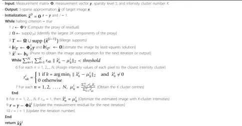
In this section, experiments were performed for validat-ing the proposed K-cluster-valued CS. For comparison, we also applied the conventional CS to exactly the same images. In all the experiments, we utilized random Gaussian matrix as the measurement matrix Fon the images. For conventional CS and K-cluster-valued CS, the maximum iteration numbers of CoSaMP were both set to be 30. Besides, the iterations can also be halted Table 1 Summary of theK-cluster-valued CoSaMP algorithm
-Input:Measurement matrixF, measurement vectory, sparsity levelS, and intensity cluster numberK.
-Output:S-sparse approximationxˆof target imagex.
-Initialization:xˆ0
=0,r=yandi= 1.
Whilehalting criterion =true
1z¬F*r{Compute the proxy of residual}
2Ω¬supp(z2K) {Identify the largest 2Kcomponents of the proxy}
3T←∪supp (xˆ(i−1)){Merge supports}
4b|T ←†
Tyandb|TC ←0{Estimate the image by least-squares solution}
5xˆi←bK{Prune to obtain the image approximation for the next iteration or output}
WhileNn=1Kk=1rnk ˆxin−μik2<threshold
6 For eachn= 1, 2,...,N, {Assign intensity values of each pixel to the closest intensity cluster}
rink=
1 ifk= arg minj ˆxin−μik2 and xˆin= 0
0 otherwise
7 For eachn= 1, 2, . . ., N, μik= Nn=1rinkˆxin
N n=1rnki
. {Obtain theKcluster centres}
End
8 Forn= 1, 2,...,N, ifrnk= 1, thenxˆin=μik{Optimize the estimated image withK-cluster intensities}
9r=y−xˆi{Update the measurement residual for the next iteration}
10i=i+ 1 {Update the iteration number}
End returnxˆxˆi
0 5 10 15 20 25 30 35
0 20 40 60 80 100 120 140 160
cluster number
image number
Figure 2 The number of images along with their optimal
cluster numbers of intensities forK-mean algorithm. Note that
the cluster number is chosen to be optimal one once it makes the
accuracy ofK-mean algorithm greater than 20 dB.
0 20 40 60 80 100 120
0 10 20 30 40 50 60 70 80
cluster number
image number
Figure 3 The number of images along with their optimal
once ˆxi− ˆxi−12 <10−2 ˆxi2. For K-cluster-valued CS, the iterative two stages ofK-means algorithm are repeated 100 times. The experiments have been per-formed under the following system environments: Matlab R2008b on a computer with Pentium(R) D 2.8-GHz CPU and 3-GB RAM. Section A focuses on utiliz-ing the K-cluster-valued and conventional CSs to com-press one lunar image relying on a canonical (pixel) sparsity basis. This subsection shows the results in detail. In Section B, we demonstrate the experiments on other extensive images in brief. This subsection mainly concentrates on the 2D images, using either a canonical sparsity basis or wavelet sparsity basis, as the input to our experiments. In addition, the experiments on some background subtracted images in color are demon-strated as well.
A One experiment in detail
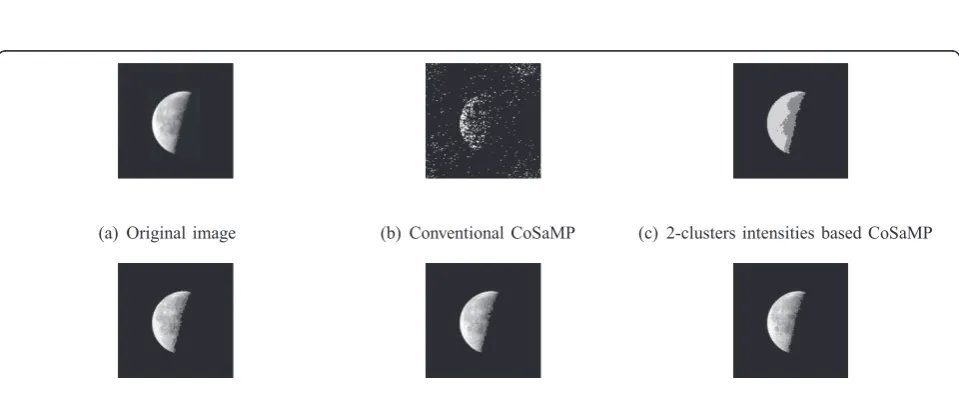
First of all, a lunar image (Figure 4a) was tested on con-ventional CS. Then, the reconstructed image is shown in Figure 4b using the recovery methods of CoSaMP, withM = 3S = 5217 random Gaussian measurements, whereS= 1739 indicates the nonzero intensity values of the lunar image. Note that the measurement numberM is approximately 13N, which is high compared to the undersampling ratio in wavelet domain. However, the advantage of the proposed and conventional CSs is that the image can be compressed directly during the acqui-sition procedure. Further, we utilized the K-cluster-valued CS to reconstruct the target lunar image given the same measurements. The recovery results are shown
in Figure 4c-f with cluster numbersK= 2, 5, 10 and 50, respectively. From Figure 4, it can be seen that when the measurements are insufficient (less than 4S), K-clus-ter-valued CS outperforms over conventional CS refer-ring to recovery accuracy. We may see that once the cluster number increases, the reconstructed images become smoother and the accuracy thus will be better. Moreover, there is almost no difference between the images reconstructed by 10-cluster and 50-cluster, and it agrees with statistical analysis of the cluster number introduced in the above section.
From the viewpoint of computational time, as can been seen from Figure 4,K-cluster-valued CS runs faster than conventional CS when cluster number Kis small (e.g.,K= 2, 5 and 10). It may be due to the fast conver-gence of K-cluster-valued CoSaMP caused by more accurate recovery result at each iteration.
Next, we shall compare the recovery error of conven-tional andK-cluster-valued CSs in terms of peak signal-to-noise ratio (PSNR). PSNR refers to the ratio between the maximum possible power of a signal and the power of corrupting noise that affects the fidelity of its repre-sentation. Since many signals have very wide dynamic ranges, PSNR is normally expressed in terms of the logarithmic decibel scale. In our experiments, PSNR, as a measure of quality of lossy image compression, is defined by:
PSNR = 20log10 255
√
N
x− ˆx2
(12)
(a) Original image (b) Conventional CoSaMP (c) 2-clusters intensities based CoSaMP
(d) 5-clusters intensities based CoSaMP (e) 10-clusters intensities based CoSaMP (f) 50-clusters intensities based CoSaMP
Figure 4(a) The original lunar gray image (resolution: 128 × 128) withS= 1,739 nonzero values. The random Gaussian measurement
number of CS over this image isM= 3S= 5,217 measurements, which is1285217×128N(∼ 13N).(b)The reconstructed image using conventional
CoSaMP recovery method.(c)-(f)The images reconstructed with 2, 5, 10 and 50 clusters of values for intensities CoSaMPs. The computational
whereN is the number of pixels at each image and 255 is the dynamic range of intensities of the image. x andxˆ are the intensities of the original image and com-pressed image, respectively.
Then, we run Monte Carlo (50 times) simulation on computing the PSNR of image reconstruction via con-ventional andK-cluster-valued CSs. The results can be seen in Figure 5. Figure 5a shows the impact of mea-surement numberM on the performance of K-cluster-valued and conventional CSs for the target image dis-played in Figure 4. Since the acceptable value for the quality of lossy image compression is above 20 dB [21], Figure 5a reveals that the proposedK-cluster-valued CS approach reaches at tolerable recovery result when M= 3S, while the conventional CS failsc. Also, it can be further seen that even when the measurement number is sufficient (M = 4S), the performance of K-cluster-valued CS is superior to conventional one. Figure 5b further shows the performance of K-cluster-valued CS given different cluster numberK. We can observe that K-cluster-valued CS works well with different cluster numbers and that the more cluster number we choose, the better K-cluster-valued CS will perform in most cases.
B More experiments in general
In this subsection, we evaluated our proposed approach on three different images sets: (1) the image set chosen from Caltech 101 database contains five images, sparse in pixel domain; (2) the natural image set contains four images, sparse or compressible in wavelet domain; (3) background subtracted color image set.
For the first image set, since we have concluded in the above section that 10 can be seen as an optimal cluster
number of intensities for the images sparse in pixel domain, we set K of K-cluster-valued CS to be 10. In addition, all the measurement numbers used for com-pressing these images were chosen to be 3S, which is less than the least measurement number 4Srequired for successful reconstruction in conventional CS [4]. Then, the reconstruction results are presented in Figure 6, and these results show the better performance of K-cluster-valued CS for compressing images that are sparse in standard domain.
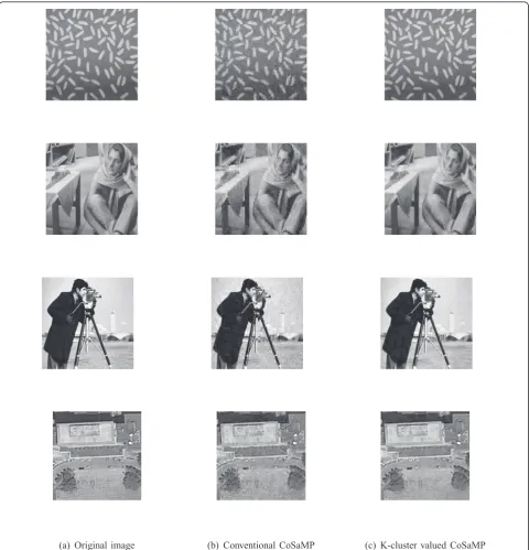
With the second image set, we have evaluated the pro-mise of the proposed CS approach on compressing the images in wavelet domain. Here, as aforementioned in Section 3, we chose the cluster number of wavelet coef-ficients forK-cluster-valued CS to be 40 as concluded in the above section. In order to obtain the more accurate results, the measurement numbers here were all set to be 3.5S, whereSis the number of largestS wavelet coef-ficients used for image reconstruction. Then, the input and output images are shown in Figure 7, and the PSNRs of the reconstructed images in this figure are further demonstrated in Table 2. Again,K-cluster-valued CS offers the better performance in compressing images, sparse in wavelet domain.
The K-clusters-valued CS is also applicable to back-ground subtracted images. Here, we tested the proposed K-clusters-valued CS and conventional CS on the third image set with two background subtraction images from [16]. According to [16], these images are obtained by selecting at random two frames of video sequence and subtracting them in a pixel-wise fashion. For each image, we set the cluster number Kto be 10 as well. Then, we performed K-clusters-valued CoSaMP and conventional CoSaMP under M= 3SGaussian random
2 2.5 3 3.5 4
14 16 18 20 22 24 26 28 30 32 34
Number of Measurements
PSNR
5−clusters based CS 50−clusters based CS Conventional CS
(a)
0 50 100 150 200
10 15 20 25 30 35
Cluster number K
PSNR
(b)
Figure 5(a) The reconstruction error of Figure 4 measured by PSNR. In this figure, the PSNR (vertical axis) is shown along with various
measurement number and the values at the horizontal axis indicate how many times of sparsity levelS.(b)The results of PSNR output byK
measurements. The recovery results are shown in Figure 8. We may see from this figure thatK-cluster-valued CS outperforms conventional one and thatK-cluster-valued CS is also capable of recovering background subtracted images with insufficient measurements (e.g., 3S measurements).
5 Conclusions
In this paper, in order to compress the image, we have aimed to propose an advanced model-based CS, named K-cluster-valued CS, which utilizes K-means algorithm as the model for CS. In contrast to conventional CS, the proposed K-cluster-valued CS incorporates the prior
knowledge that only Kclusters values of intensities are available for all the pixels of an image. In this paper, we also investigated cluster numberKas prior knowledge. Such prior knowledge goes beyond the simple sparsity/ compressibility of CS and therefore has the advantage in using fewer measurements than conventional CS for accurate image reconstruction. This way, K-cluster-valued CS is applicable to other K-cluster-valued signals (e.g., binary digital signals) besides the images. Also, it is applicable to other model-based CS by considering all the prior knowledge together. Moreover, the experi-ments were performed and presented to validate the proposed approach.
.
(a) Original image (b) Conventional CoSaMP (c) 10-cluster intensities valued
CoSaMP
Figure 6(a) The original gray images. The measurement numbers of both conventional andK-cluster-valued CS over these images areM=
3S, whereSis the sparse level.(b)The reconstructed images using conventional CoSaMP recovery method.(c)The images reconstructed byK
Endnotes
a
This is the usual case since an image is normally com-prised of a few categories of objects with limited color intensities as exploited in computer vision community. b
The Kclusters can also be applied in color image by extending each gray valuexˆi
nto be 3 space comprising
(a) Original image (b) Conventional CoSaMP (c) K-cluster valued CoSaMP
Figure 7(a) The original gray images measured by CS with wavelet sparsity basis. The measurement numbers of both conventional and
K-cluster-valued CS over these images areM= 3.5S, whereSis the number of compressible wavelet coefficients greater than threshold 20.(b)
The reconstructed images using the conventional CoSaMP recovery method.(c)The images reconstructed byK-cluster-valued (wavelet
coefficients) CoSaMP. Note that cluster numberKwas chosen to be 40 for all these images.
Table 2 The PSNRs of reconstructed images of Figure 7
Methods (a) (b) (c) (d)
Conventional CoSaMP 22.61 22.10 20.85 21.67
the intensities of the red, blue and green channels.cIt is due to the fact that conventional CS does not have any prior knowledge of the range of intensity values of the pixels.
Acknowledgements
This work was partially supported by China National Basic Research Program (973) under Grant number 2007CB310600 and partially supported by NSFC 30971689.
Competing interests
The authors declare that they have no competing interests.
Received: 18 February 2011 Accepted: 26 September 2011 Published: 26 September 2011
References
1. M Petrou, C Petrou,Image Processing: The Fundamentals, 2nd edn. (Wiley,
Amsterdam, 2010)
2. S Mallat,A Wavelet Tour of Signal Processing(Academic Press, New York,
1999)
3. D Taubman, M Marcellin,JPEG 2000: Image Compression Fundamentals,
Standards and Practice, 1st edn. (Kluwer Academic, Dordrecht, 2001)
4. E Candès, M Wakin, An introduction to compressive sampling. IEEE Signal
Process Mag.25(2), 21–30 (2008)
5. E Candès, J Romberg, T Tao, Robust uncertainty principles: exact signal
reconstruction from highly incomplete frequency information. IEEE Trans Inf
Theory.52(02), 489–509 (2006)
6. E Candès, T Tao, Near-optimal signal recovery from random projections:
Universal encoding strategies?. IEEE Trans Inf Theory52(12), 5406–5425
(2006)
7. D Donoho, Compressed sensing. IEEE Trans Inf Theory.52(4), 1289–1306
(2006)
8. E Candès, J Romberg, T Tao, Stable signal recovery from incomplete and
inaccurate measurements. Commun Pure Appl Math.59(8), 1207–1223
(2006). doi:10.1002/cpa.20124
9. S Boyd, L Vandenberghe,Convex Optimization(Cambridge University Press,
Cambridge, 2004)
10. J Tropp, A Gilbert, Signal recovery from random measurements via
orthogonal matching pursuit. IEEE Trans Inf Theory.53(12) 267–288 (2007)
11. DL Donoho, Y Tsaig, I Drori, J luc Starck, Sparse solution of
under-determined linear equations by stagewise orthogonal matching pursuit.
Tech Rep, March, 1–39 (2006)
12. W Dai, O Milenkovic, Subspace pursuit for compressive sensing signal
reconstruction. IEEE Trans Inf Theory55(5), 267–288 (2009)
13. D Needell, J Tropp, Cosamp: iterative signal recovery from incomplete and
inaccurate samples. Appl Comput Harmon Anal.26(3), 301–321 (2009).
doi:10.1016/j.acha.2008.07.002
14. R Baraniuk, V Cevher, M Duarte, C Hegde, Model-based compressive
sensing. IEEE Trans Inf Theory56(4), 1982–2001 (2010)
15. Y Eldar, P Kuppinger, H Bolcskei, Compressed sensing of block-sparse
signals: uncertainty relations and efficient recovery. IEEE Trans Signal Process (2009)
16. V Cevher, M Duarte, C Hegde, R Baraniuk, Sparse signal recovery using
markov random fields, inProceedings of NIPS(2008)
17. V Cevher, P Indyk, H Chinmay, R Baraniuk, Recovery of clustered sparse
signals from compressive measurements, inProceedings of Sampta09(2009)
18. CM Bishop,Pattern Recognition and Machine Learning, 1st edn. (Springer,
New York, 2006)
19. T Blumensath, M Davies, Sampling theorems for signals from the union of
finite-dimensional linear subspaces. IEEE Trans Inf Theory55(4), 1872–1882
(2008)
20. SP Lloyd, Least squares quantization in pcm. IEEE Trans Inf Theory28(2),
129–136 (1982). doi:10.1109/TIT.1982.1056489
21. N Thomos, N Boulgouris, M Strintzis, Optimized transmission of jpeg2000
streams over wireless channels. IEEE Trans Image Process15(1), 54–67
(2006)
doi:10.1186/1687-6180-2011-75
Cite this article as:Xu and Lu:K-cluster-valued compressive sensing for imaging.EURASIP Journal on Advances in Signal Processing20112011:75.
Submit your manuscript to a
journal and benefi t from:
7Convenient online submission 7Rigorous peer review
7Immediate publication on acceptance 7Open access: articles freely available online 7High visibility within the fi eld
7Retaining the copyright to your article
Submit your next manuscript at 7 springeropen.com
.
(a) Original image (b) Conventional CoSaMP (c) 10-clusters intensities valued
CoSaMP
Figure 8(a) Two original background subtraction images. The recovery results are shown in(b)for conventional CS and(c)forK