Volume 2007, Article ID 87046,22pages doi:10.1155/2007/87046
Research Article
Design and Implementation of Numerical Linear Algebra
Algorithms on Fixed Point DSPs
Zoran Nikoli´c,1Ha Thai Nguyen,2and Gene Frantz3
1DSP Emerging End Equipment, Texas Instruments Inc., 12203 SW Freeway, MS722, Stafford, TX 77477, USA
2Coordinated Science Laboratory, Department of Electrical and Computer Engineering,
University of Illinois at Urbana-Champaign, 1308 West Main Street, Urbana, IL 61801, USA
3Application Specific Products, Texas Instruments Inc., 12203 SW Freeway, MS701, Stafford, TX 77477, USA
Received 29 September 2006; Revised 19 January 2007; Accepted 11 April 2007
Recommended by Nicola Mastronardi
Numerical linear algebra algorithms use the inherent elegance of matrix formulations and are usually implemented using C/C++ floating point representation. The system implementation is faced with practical constraints because these algorithms usually need to run in real time on fixed point digital signal processors (DSPs) to reduce total hardware costs. Converting the simulation model to fixed point arithmetic and then porting it to a target DSP device is a difficult and time-consuming process. In this paper, we analyze the conversion process. We transformed selected linear algebra algorithms from floating point to fixed point arithmetic, and compared real-time requirements and performance between the fixed point DSP and floating point DSP algorithm implementations. We also introduce an advanced code optimization and an implementation by DSP-specific, fixed point C code generation. By using the techniques described in the paper, speed can be increased by a factor of up to 10 compared to floating point emulation on fixed point hardware.
Copyright © 2007 Zoran Nikoli´c et al. This is an open access article distributed under the Creative Commons Attribution License, which permits unrestricted use, distribution, and reproduction in any medium, provided the original work is properly cited.
1. INTRODUCTION
Numerical analysis motivated the development of the earli-est computers. During the last few decades linear algebra has played an important role in advances being made in the area of digital signal processing, systems, and control [1]. Numer-ical algebra tools—such as eigenvalue and singular value de-composition, least squares, updating and downdating—are an essential part of signal processing [2], data fitting, Kalman filters [3], and vision and motion analysis. Computational and implementational aspects of numerical linear algebraic algorithms have strongly influenced the ways in which com-munications, computer vision, and signal processing prob-lems are being solved. These algorithms depend on high data throughput and high speed computations for real-time per-formance.
DSPs are divided into two broad categories: fixed point and floating point [4]. Numerical algebra algorithms often rely on floating point arithmetic and long word lengths for high precision, whereas digital hardware implementations of these algorithms need fixed point representation to reduce total hardware costs. In general, the cutting-edge, fixed point families tend to be fast, low power and low cost, while
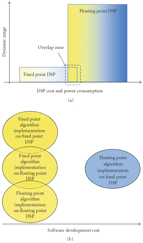
float-ing point processors offer high precision and wide dynamic range. Fixed point DSP devices are preferred over floating point devices in systems that are constrained by chip size, throughput, price-per-device, and power consumption [5]. Fixed point realizations vastly outperform floating point re-alizations with regard to these criteria.Figure 1shows a chart on how DSP performance has increased over the last decade. The performance in this chart is characterized by number of multiply and accumulate (MAC) operations that can execute in parallel. The latest fixed point DSP processors run at clock rates that are approximately three times higher and perform four times more 16×16 MAC operations in parallel than floating point DSPs.
Therefore, there is considerable interest in making float-ing point implementations of numerical linear algebra algo-rithms amenable to fixed point implementation. In this pa-per, we investigate whether the fixed point DSPs are capable of handling linear numerical algebra algorithms efficiently and accurately enough to be effective in real time, and we look at how they compare to floating point DSPs.
1996 1997 1998 1999 2000 2001 2002 2003 2004 2005 2006 2007 Year
102 103 104 105
(M
illions
o
f
m
ultiply
and
ac
cum
ulat
e
oper
ations)/S
Fixed point DSP Floating point DSP TMS320C6701
TMS320C6711
TMS320C6713 TMS320C67x+ TMS320C62x
TMS320C64x
TMS320C64x+
Figure1: DSP performance trend.
floating point and extended-precision fixed point allows de-signers to balance dynamic range and precision on an as-needed basis, thus giving them a new level of control over DSP system implementations. The overlap between fixed point and floating point DSPs is shown inFigure 2(a).
The modeling efficiency level on the floating point is high and the floating point models offer a maximum degree of reusability. Converting the simulation model to fixed point arithmetic and then porting it to a target device is a time con-suming and difficult process. DSP devices have very different instruction sets, so an implementation on one device cannot be ported easily to another device if it fails to achieve suffi-cient quality. Therefore, development cost tends to be lower for floating point systems (Figure 2(b)).
Designers with applications that require only minimal amounts of floating point functionality are caught in an “overlap zone,” and they are often forced to move to higher-cost floating point devices. Today however, fixed point pro-cessors are running at high enough clock speeds for designer to combine floating point emulation and fixed point arith-metic in order to meet real-time deadlines. This allows a tradeoffbetween computational efficiency of floating point and low cost and low power of fixed point. In this paper, we are trying to extend the “overlap zone” and we investigate fixed point implementation of a truly float-intensive applica-tion, such as numerical linear algebra.
A typical design flow of a floating point system targeted for implementation on a floating point DSP is shown in Figure 3.
The design flow begins with algorithm implementation in floating point on a PC or workstation. The floating point system description is analyzed by means of simulation with-out taking the quantization effects into account. The mod-eling efficiency on the floating point level is high and the floating point models offer a maximum degree of
reusabil-Floating point DSP
Fixed point DSP
DSP cost and power consumption Overlap zone
Dynamic
range
(a)
Fixed point algorithm implementation
on fixed point DSP Fixed point
algorithm implementation on floating point
DSP Floating point
algorithm implementation on floating point
DSP
Floating point algorithm implementation
on fixed point DSP
Software development cost (b)
Figure2: Fixed point and floating point DSP pros and cons.
PC
or
wo
rk
st
at
io
n
de
ve
lopment
en
vi
ro
nment
DSP/target deve
lopment
en
vi
ro
nment
Mapping of a floating point algorithm to a floating point
DSP target Floating point
algorithm implementation
DSP-specific optimizations
Ok?
Figure3: Floating point design process.
PC
or
wo
rk
st
at
io
n
de
ve
lopment
en
vi
ro
nment
DSP/target deve
lopment
en
vi
ro
nment
Floating point algorithm implementation
Only critical sections are selected for conversion to fixed point
Ok?
Quantization/ bit-true fixed
point algorithm implementation
System partitioning
Mapping of the fixed point algorithm to a fixed point DSP
target DSP-specific optimizations Range estimation
OK? The partitioning
is based on performance
Bit-true fixed point simulation
(e.g., in systemC)
Figure4: Fixed point design process.
There are several program languages and block diagram-based CAD tools that support fixed point data types [6,8], but C language is still more flexible for the development of digital signal processing programs containing machine vision and control intensive algorithms. Therefore, design flow— in a case when the floating point implementation needs to be mapped to fixed point—is more complicated for two rea-sons:
(i) it is difficult to find fixed point system representa-tion that optimally maps to system model developed in floating point;
(ii) C/C++ does not support fixed point formats. Model-ing of a bit-true fixed point system in C/C++ is diffi -cult and slow.
A previous approach to alleviate these problems when target-ing fixed point DSPs was to use floattarget-ing point emulation in a high level C/C++ language. In this case, design flow is very similar to the flow presented inFigure 3, with the difference that the target is a fixed point DSP. However, this method sac-rifices severely the execution speed because a floating point operation is compiled into several fixed point instructions. To solve these problems, a flow that converts a floating point C/C++ algorithm into a fixed point version is developed.
A typical fixed point design flow is depicted inFigure 4. To speed up the porting process, only the most time con-suming floating point functions can be converted to fixed
point arithmetic. The system is divided into subsections and each subsection is benchmarked for performance. Based on the benchmark results functions critical to system per-formance are identified. To improve overall system perfor-mance, only the critical floating point functions can be con-verted to fixed point representation.
In a next step towards fixed point system implementa-tion, a fixed exponent is assigned to every operand. Deter-mining the optimum fixed point representation can be time-consuming if assignments are performed by trial and error. Often more than 50% of the implementation time is spent on the algorithmic transformation to the fixed point level for complex designs once the floating point model has been specified [9]. The major reasons for this bottleneck are the following:
(i) the quantization is generally highly dependent on the stimuli applied;
(ii) analytical methods for evaluating the fixed point per-formance based on signal theory are only applicable for systems with a low complexity [10]. Selecting opti-mum fixed point representation is a nonlinear process, and exploration of the fixed point design space cannot be done without extensive system simulation;
The bit-true fixed point system model is run on a PC or a work station. For efficient modeling of fixed point bit-true system representation, language extensions implement-ing generic fixed point data types are necessary. Fixed point language extensions implemented as libraries in C++ of-fer a high modeling efficiency [10,11]. The libraries supply generic fixed point data types and various casting modes for overflow and quantization handling and some of them also offer data monitoring capabilities during simulation time. The simulation speed of these libraries on the other hand is rather poor.
After validation on a PC or workstation, the quan-tized bit-true system is intended for implementation in soft-ware on a programmable fixed point DSP. The implementa-tion needs to be optimized with respect to memory utiliza-tion, throughput, and power consumption. Here the bit-true system-level model developed during quantization serves as a “golden” reference for the target implementation which yields bit-by-bit the same results.
Memory, throughput, and word length requirements may not be important issues for off-line implementation of the algorithms, but they can become critical issues for real-time implementations in embedded processors—especially as the system dimension becomes larger [3,12]. The load that numerical linear algebra algorithms place on real-time DSP implementation is considerable. The system implementation is faced with the practical constraints. Meaningful measures of this load are storage and computation time. The first item impacts the memory requirements of the DSP, whereas the second item helps to determine the rate at which measure-ments can be accepted. To reach a high level of efficiency, the designer has to keep the special requirements of the DSP tar-get in mind. The performance can be improved by matching the generated code to the target architecture.
The platforms we chose for this evaluation were Very Long Instruction Word (VLIW) DSPs from Texas Instru-ments. For evaluation of the fixed point design flow we used the C64x+ fixed point CPU core. To evaluate floating point DSP performance we used C67x and C67x+ floating point CPU cores. Our goals were to identify potential numerical algebra algorithms, to convert them to fixed point, and to evaluate their numerical stability on the fixed point of the C64x+. We wanted to create efficient C implementations in order to test whether the C64x+ is fast and accurate enough for this task, and finally to investigate how fixed point real-ization stacks up against the algorithm implementation on a floating point DSP.
In this paper, we present methods that address the chal-lenges and requirements of fixed point design process. The flow proposed is targeted at converting C/C++ code with floating point operations into C code with integer operations that can then be fed through the native C compiler for var-ious DSPs. The proposed flow relies on the following main concepts:
(i) range estimation utility used to determine fixed point format. The range estimation software tool presented in this paper, semiautomatically transforms numerical linear algebra algorithms from C/C++ floating point
to a bit-true fixed point representation that achieves maximum accuracy. Difference between this tool and existing tools [5,9,13–15] is discussed inSection 3; (ii) software tool support for generic fixed point, data
types. This allows modeling of the fixed point behavior of the system. The bit-true fixed point model is simu-lated and finely tuned on PC or a work station. When desired precision is achieved, the bit-true fixed point is ported to a DSP;
(iii) seamless design flow from bit-true fixed point simu-lation on PC down to system implementation, gener-ating optimized input for DSP compilers. The maxi-mum performance is achieved by matching the gener-ated code to the target architecture.
The remainder of this paper is organized as follows: the next subsection gives a brief overview of fixed point arithmetic; Section 2gives a background on the numerical linear alge-bra algorithms selection;Section 3presents dynamic range estimation process;Section 4presents the quantization and bit-true fixed point simulation tools.Section 5gives a brief overview of DSP architecture and presents tools for DSP-specific optimization and implementation. Results are dis-cussed inSection 6.
1.1. Fixed point arithmetic
In case of the 32-bit data, the binary point is assumed to be located to the right of bit 0 for an integer format, whereas for a fractional format it is next to the bit 31, the sign bit. It is difficult to represent all the data satisfactorily just by using in-teger of fractional numbers. The generalized fixed point for-mat allows arbitrary binary point location. The binary point is also calledQpoint.
We use the standardQnotationQnwherenis the num-ber of fractional bits. The total size of the numnum-ber is as-sumed to be the nearest power of 2 greater than or equal to n, or clear from the context unless it is explicitly spelled out. Hence “Q15” refers to a 16-bit signed short with a thought comma point to the right of the leftmost bit. Likewise, an “unsigned Q32” refers to a 32-bit unsigned integer with a thought comma point directly to the left of the leftmost bit. Table 1summarizes the range of 32-bit fixed point number for differentQformat representations.
In this format, the location of the binary point, or the integer word length, is determined by the statistical magni-tude, or range of signal not to cause overflows. Since each signal can have a different value for the range, a unique in-teger word length can be assigned to each variable. For ex-ample, one sign bit, two integer bits and 29 fractional bits can be allocated for the representation of a signal having dy-namic range of [−4, 3.999999998]. This means that the bi-nary point is assumed to be located two bits below the sign bit. The format not only prevents overflows, but also has a small quantization level 2−29.
Table1: Range of 32-bit fixed point number for differentQformat representations.
Type Range Type Range
Min Max Min Max
IQ30 −2 1.999 999 999 IQ15 −65536 65535.999 969 482
IQ29 −4 3.999 999 998 IQ14 −131072 131071.999 938 965
IQ28 −8 7.999 999 996 IQ13 −262144 262143.999 877 930
IQ27 −16 15.999 999 993 IQ12 −524288 524287.999 755 859 IQ26 −32 31.999 999 985 IQ11 −1048576 1048575.999 511 719 IQ25 −64 63.999 999 970 IQ10 −2097152 2097151.999 023 437 IQ24 −128 127.999 999 940 IQ9 −4194304 4194303.998 046 875 IQ23 −256 255.999 999 981 IQ8 −8388608 8388607.996 093 750 IQ22 −512 511.999 999 762 IQ7 −16777216 16777215.992 187 500 IQ21 −1024 1023.999 999 523 IQ6 −33554432 33554431.984 375 000 IQ20 −2048 2047.999 999 046 IQ5 −67108864 67108863.968 750 000 IQ19 −4096 4095.999 998 093 IQ4 −134217728 134217727.937 500 000 IQ18 −8192 8191.999 996 185 IQ3 −268435456 268435455.875 000 000 IQ17 −16384 16383.999 992 371 IQ2 −536870912 536870911.750 000 000 IQ16 −32768 32767.999 984 741 IQ1 −1073741824 1 073741823.500 000 000
the integer word length can be changed by using arithmetic shift. An arithmetic right shift of n-bit corresponds to in-creasing the integer word length byn. The output of multi-plication has the integer word length which is sum of the two input integer word lengths, assuming that one superfluous sign bit generated in the two’s complement multiplication is deleted by one left shift.
For a bit-true and implementation independent specifi-cation of a fixed point operand, a three-tuple is necessary: the word length WL, theinteger word length IWL, and thesign S. For every fixed point format, two of the three parametersWL, IWL, andFWL(fractional word length) are independent; the third parameter can always be calculated from the other two, WL = IWL + FWL. Note that aQ0 data type is merely a spe-cial case of a fixed point data type with anIWLthat always equalsWL—hence an integral data type can be described by two parameters only, the word lengthWLand the sign encod-ingS(an integral data typeQ0 is not presented inTable 1).
2. LINEAR ALGEBRA ALGORITHM SELECTION
The vitality of the field of matrix computation stems from its importance to a wide area of scientific and engineering ap-plications on the one hand, and the advances in computer technology on the other. An excellent, comprehensive refer-ence on matrix computation is Golub and van Loan’s text [16].
Commercial digital signal processing applications are constrained by the dictates of real-time implementations. Usually a big part of the DSP bandwidth is allocated for com-putationally intensive matrix factorizations [17,18]. As the processing power of DSPs keeps increasing, more of these al-gorithms become practical for real-time implementation.
Five algorithms were investigated: Cholesky decomposi-tion, LU decomposition with partial pivoting,QR
decom-position, Jacobi singular-value decomdecom-position, and Gauss-Jordan algorithm.
These algorithms are well known and have been exten-sively studied, and efficient and accurate floating point im-plementations exist. We want to explore their implementa-tion in fixed point and compare it to floating point.
3. PROCESS OF DYNAMIC RANGE ESTIMATION
3.1. Related work
During conversion from floating point to fixed point, a range of selected variables is mapped from floating point space to fixed point space. Some published approaches for floating point to fixed point conversion use an analytic approach for range and error estimation [9, 13,19–23], and others use a statistical approach [5,11,24,25]. After obtaining mod-els or statistics of range and error by analytic or statistical approaches, respectively, search algorithms can find an opti-mum word length. A useful survey and comparison of search algorithms for word length determination is presented in [26].
The advantages of analytic techniques are that they do not require simulation stimulus and can be faster. However, they tend to produce more conservative word length results. The advantage of statistical techniques is that they do not re-quire a range or error model. However, they often need long simulation time and tend to be less accurate in determining word lengths. After obtaining models or statistics of range and error by analytic or statistical approaches, respectively, search algorithms can find an optimum word length.
of adaptive or nonlinear systems. The range estimation based upon L1 norm analysis is applicable only to specific signal processing algorithms (e.g., adaptive lattice filters [28]). Op-timum word length choices can be made by solving equations when propagated quantized errors [29] are expressed in an analytical form.
Other analytic approaches use a range and error model for integer word length and fractional word length design. Some use a worst-case error model for range estimation [19,23], and some use forward and backward propagation forIWLdesign [21]. Still others use an error model forFWL [15,19].
By profiling intermediate calculation results within ex-pression trees-in addition to values assigned to explicit pro-gram variables, a more aggressive scaling is possible than those generated by the “worst case estimation” technique de-scribed in [9]. The latter techniques begin with range infor-mation for only the leaf operands of an expression tree and then combine range information in a bottom up fashion. A “worst-case estimation” analysis is carried out at each opera-tion whereby the maximum and minimum result values are determined from the maximum and minimum values of the source operands. The process is tedious and requires the de-signer to bring in his knowledge about the system and specify a set of constraints.
Some statistical approaches use range monitoring for IWLestimation [11,24], and some use error monitoring for FWL[22,24]. The work in [22] also uses an error model that has coefficients obtained through simulation.
In the “statistical” method presented in [11], the mean and standard deviation of the leaf operands are profiled as well as their maximum absolute value. Stimuli data is used to generate a scaling of program variables, and hence leaf operands, that avoid overflow by attempting to predict from the signal variances of leaf operands whether intermediate results will overflow.
During the conversion process of floating point numeri-cal linear algebra algorithms to fixed point, the integer word length (IWL) part and the fractional word length (FWL) part are determined by different approaches while architecture word length (WL) is kept constant. In case when a fixed point DSP is target hardware,WLis constrained by the CPU archi-tecture.
Float to fixed conversion method, used in this paper, originates in simulation-based, word length optimization for fixed point digital signal processing systems proposed by Kim and Sung [5] and Kim et al. [11]. The search algorithm at-tempts to find the cost-optimal solution by using “exhaus-tive” search. The technique presented in [11] requires mod-erate modification of the original floating point source code, and does not have standardized support for range estimation of multidimensional arrays.
The method presented here, unlike work in [5,11], is minimally intrusive to the original floating point C/C++ code and has a uniform way to support multidimensional arrays and pointers which are frequently used in numerical linear algebra. The range estimation approach presented in the subsequent section offers the following features:
(i) minimum code intrusion to the original floating point C model. Only declarations of variables need to be modified. There is also no need to create a secondary main()function in order to output simulation results; (ii) support for pointers and uniform standardized sup-port for multidimensional arrays which are frequently used in numerical linear algebra;
(iii) during simulation, key statistical information and value distribution of each variable are maintained. The distribution is kept in a 32-bin histogram where each bin corresponds to oneQformat;
(iv) output from the range-estimation tool is split in dif-ferent text files on function by function basis. For each function, the range-estimation tool creates a separate text file. Statistical information for all tracked variables within one function is grouped together within a text file associated to the function. The output text files can be imported in Excel spreadsheet for review.
3.2. Dynamic range estimation algorithm
The semiautomated approach proposed in this section uti-lizes simulation-based profiling to excite internal signals and obtain reliable range information. During the simulation, the statistical information is collected for variables speci-fied for tracking. Those variables are usually the floating point variables which are to be converted to fixed point. The statistics collected is the dynamic range, the mean and standard deviation and the distribution histogram. Based on the collected statistic information Qpoint location is sug-gested.
The range estimation can be performed on function-by-function basis. For example, only a few of the most time consuming functions in a system can be converted to fixed point, while leaving the remaining of the system in floating point.
The method is minimally intrusive to the original float-ing point C/C++ code and has uniform way of support for multidimensional arrays and pointers. The only modifica-tion required to the existing C/C++ code is marking the vari-ables whose fixed point behavior is to be examined with the range estimation directives. The range estimator then finds the statistics of internal signals throughout the floating point simulation using real inputs and determines scaling parame-ters.
· · ·
ti floatX
Static member: VarList (a linked list of statistics):
· · ·
ti floatY ti floatZ Statisticsx Statisticsy Statisticsz
Update stats
Update stats
Update stats ti float class
Figure5:ti floatclass composition.
Classstatisticsare used to keep track of the minimum, maximum, standard deviation, overflow, underflow and his-togram of floating point variable associated with it. All in-stances of class statistics are stored in a linked-list class VarList. The linked list VarList is a static member of class ti float. Every time a new variable is declared as a ti float, a new object of classstatisticsis created. The new statistics object is linked to the last element in the linked listVarList, and associated with the variable. Statistics information for all floating point variables declared asti floatis tracked and recorded in the VarList linked list. By declaring linked list of statistics objects as a static member of class ti float we achieved that every instance of the objectti floathas access to the list. This approach minimizes intrusion to the origi-nal floating point C/C++ code. Structure of classti float is shown inFigure 5.
Every time a variable, declared as ti float, is assigned a value during simulation, in order to update the variable statistics, the ti float class searches through the linked list VarList for thestatisticsobject which was associated with the variable.
The declaration of a variable asti floatalso creates asso-ciation between the variable name and function name. This association is used to differentiate between variables with same names in different functions. Pointers and arrays, as frequently used in ANSI C, are supported as well.
Declaration syntax forti floatis
ti float<var name>(“<funct name>,””<var name>”);
where<var name>is the name of floating point variable des-ignated for dynamic range tracking, and<funct name>is the name of function where the variable is declared.
In case dynamic range of multidimensional array of float needs to be determined, the array declaration must be changed from
float<var name>[<M>][<N>]· · ·[<Z>];
to
ti float<var name>[<M>][<N>]· · ·[<Z>] ={ti float(“<funct name>,””<var name>,”
<M>∗<N>∗· · ·∗<Z>)}.
Please note that declaration of multidimensional array of ti float can be uniformly extended to any dimension. The declaration syntax keeps the same format for one, two, three, andndimensional array ofti float. In the declaration <var name>is the name of floating point array selected for dynamic range tracking. The <func name>is the name of function where the array is declared. The third element in the declaration of array ofti floatis size. Array size is defined by multiplying sizes of each array dimension.
In case of multidimensionalti floatarrays only one statis-ticsobject is created to keep track of statistics information of the whole array. In other words,ti floatclass keeps statistic information for array at array level and not for each array el-ement. Product defined as third element in the declaration defines the array size.
Theti floatclass overloads arithmetic and relational op-erators. Hence, basic arithmetic operations such as addition, subtraction, multiplication, and division are conducted au-tomatically for variables. This property is also applicable for relational operators, such as “==,” “>,” ”<,“ ”>=,“”!=“ and “<=.” Therefore, anyti floatinstance can be compared with floating point variables and constants. The contents, or pri-vate members, of a variable declared by the class are updated when the variable is assigned by one of the assignment op-erators, such as “=,” “+ =,” “− =,” “∗ =,” and “/ =.” For example,ti floatis updated when the absolute of the present value is larger than the previously determined.
The floating point simulation model is prepared for range estimation by changing the variable declaration from float to ti float. The simulation model code must be com-piled and linked with the overloaded operators of theti float class. The Microsoft Visual C++ compiler, version 6.0, is used throughout the floating point and range estimation develop-ment.
The dynamic range information is gathered during the simulation for each variable declared asti float. The statisti-cal range of a variable is estimated by using histogram, stan-dard deviation, minimum and maximum values. Finally, the integer word lengths of all signals declared asti floatare sug-gested.
(1) void choldc(float **a, int n, float p[]) (2){
(3) void nrerror(char error text[]); (4) int i,j,k;
(5) float sum; (6)
(7) for (i=0;i<n;i++){ (8) for (j=i;j<n;j++){
(9) for (sum=a[i][j],k=i-1;k>=1;k- -) sum -=a[i][k]*a[j][k]; (10) if (i==j){
(11) if (sum<=0.0)
(12) nrerror(“choldc failed”); (13) p[i]=sqrt(sum);
(14) }else a[j][i]=sum/p[i];
(15) }
(16) } (17)}
Figure6: Floating point code for Cholesky decomposition.
in which the assigned value can be represented with mini-mumIWL is selected. The decision is made based on his-togram data collected during simulation.
In this case, large floating point dynamic range is mapped to one of 31 possible fixed point formats fromTable 1. To identify the best fixed point format the variable values are tracked by using a histogram with 32 bins. Each of these bins present one Q format. Every time during simulation, the tracked floating point variable is assigned a value, a corre-spondingQformat representation of the value is calculated and the value is binned to a correspondingQpoint bin. In case floating point value is too large to be presented in 32-bit fixed point it is sorted in the Overflow bin. In case floating point value is too small to be presented in 32-bit fixed point it is sorted in the Underflow bin.
At the end of simulation,ti float objects save collected statistics in a group of text files. Each text file corresponds to one function, and contains statistic information for variables declared asti floatwithin that function.
Cholesky decomposition is used to illustrate porting from floating point to fixed point arithmetic. The overall procedure to estimate the ranges of internal variables can be summarized as follows.
(1) Implement Cholesky decomposition in floating point arithmetic C/C++ program. Floating point implementa-tion of Cholesky decomposiimplementa-tion is presented in Figure 6 [30].
(2)Insert the range estimation directives.In this case dy-namic range is tracked for all floating point variables de-clared in choldc() function. Dynamic range of float vari-able sum, two-dimensional array of floatsa[][], and one-dimensional float arrayp[] are traced. Declarations for these variables are changed from float toti floatas shown in lines (5), (7), and (8) shown in Figure 7. In line (7), a two-dimensional array ofti floatis declared. The declaration as-sociates the name of two-dimensional array “a” with func-tion name “choldc.”
Note that declaration of ti float can be uniformly ex-tended for multidimensional arrays.
(3)Rebuild model and run. Code must be linked with li-brary containing theti floatimplementation. During simu-lation, statistic data is collected for all variables declared as ti float. After the simulation is complete, the collected data is saved in a group of text files. A text file is associated with each function. All variables declared asti floatwithin a function are grouped and saved together. In this case, data associated to tracked variables from functioncholdc()are saved in text file namedcholdc.txt. Content of thecholdc.txt is shown in Figure 8.
Statistics collected for each variable is presented in sepa-rate rows. In rows (7), (8), and (9) statistics for variablesp, a, andsum are presented. TheQpoint information shown in column B presentsQformat suggestion. For example, the tool suggestsQ28 format for elements of two-dimensional arraya. The count information, shown in column C, presents how many times particular variable was assigned a value dur-ing course of simulation. The information shown in columns D through I inFigure 8, respectively, present
(i) Min: smallest value of the selected variable during sim-ulation;
(ii) Max: largest value of the selected variable during sim-ulation;
(iii) Abs Min: absolute smallest value of the selected vari-able during simulation;
(iv) Abs Max: absolute largest value of the selected variable during simulation;
(v) Mean: mean value of the selected variable during sim-ulation;
(vi) Std dev:standard deviation value of the selected vari-able during simulation.
(1) choldc(float **ti a, int n, float ti p[]) (2){
(3) int i,j,k; (4)
(5) ti float sum(“choldc,” “sum”); (6)
(7) ti float a[M][M]={ti float(“choldc,” “a,” M*M)}; (8) ti float p[M]={ti float(“choldc,” “p,” M)}; (9)
(10) for (i=0; i<n; i++) (11) {
(12)
(13) for (j=0; j<n; j++) a[i][j]=ti a[i][j]; (14) }
(15)
(16) for (i=0;i<n;i++){ (17) for (j=i;j<n;j++){
(18) for (sum=a[i][j],k=i-1;k>=0;k- -) sum -=a[i][k]*a[j][k]; (19) if (i==j){
(20) if (sum<=0.0)
(21) nrerror(“choldc failed”); (22) p[i]=sqrt(sum);
(23) }else a[j][i]=sum/p[i];
(24) }
(25) } (26)
(27) for (i=0; i<n; i++) (28) {
(29) ti p[i]=p[i];
(30) for (j=0; j<n; j++) ti a[i][j]=a[i][j]; (31) }
(32)}
Figure7: Floating point code for Cholesky decomposition prepared for range estimation.
Figure8: Output from range estimation tool imported in excel spreadsheet.
course of simulation variablesumtook twice values that can be represented inQ28 fixed point format, it took 100 times values that can be represented inQ29 fixed point format and it took 458 times values that can be represented inQ29 fixed point format. Overflow and Underflow bins track number of overflows and underflows, respectively.
4. BIT-TRUE FIXED POINT SIMULATION
fixed point code to a DSP platform. Cosimulating this fixed point algorithm with the original floating point code will give an accuracy evaluation.
Since ANSI C or C++ offers no efficient support for fixed point data types, it is not possible to easily carry the fixed point simulation in pure ANSI C or C++. Several library ex-tensions to C++ have been proposed in the past to compen-sate for this deficiency [7,31]. These fixed point language extensions are implemented as libraries in C++ and offer a high modeling efficiency. They supply generic fixed point data types and various casting modes for overflow and quan-tization handling. The simulation speed of these libraries on the other hand is rather poor.
The SystemC fixed point data types and cast operators are utilized in proposed design flow [7]. Since ANSI C is a subset of SystemC, the additional fixed point constructs can be used as bit-true annotations to dedicated operands of the original floating point ANSI C file, resulting in ahybridspecification. This partially fixed point code is used for simulation.
In the following paragraphs, a short overview of the most frequently used fixed point data types and functions in Sys-temC is provided. A more detailed description can be found in the SystemC user’s manual [7].
The data typessc fixed andsc ufixedare the data types of choice. The two’s complement data typesc fixedand the unsigned data typesc ufixedreceive their format when they are declared, that is, the fixed point attributes must be known at compile time (static arguments). Thus they behave accord-ing to these fixed point parameters throughout their lifetime. Pointers and arrays, as frequently used in ANSI C, are sup-ported as well.
For a cast operation to a fixed point format<WL, IWL, SIGN>, it is also important to specify the overflow and pre-cision reduction in case the target data type cannot hold the original value. The most important casting modes are listed below. SystemC also specifies many additional cast modes to model target specific behavior.
(i) Quantization modes
(a)Truncation(SC TRN). The bits below the spec-ified LSB are cut off. This quantization mode is the default for SystemC fixedpoint types and will be used if no other value is specified.
(b)Rounding (SC RND). Adds LSB/2 first, before cutting offthe bits below the LSB.
(ii)Overflow modes
(a)Wrap-around(SC WRAP). In case of an overflow the MSB carry bit is ignored. This overflow mode is the default for SystemC fixed point types and will be used if no other value is specified. (b)Saturation (SC SAT). In case the minimum or
maximum values are exceeded, the result is set to the minimum or maximum values, respectively.
Described above are thealgorithmic leveltransformations as illustrated inFigure 9, that change the behavior or accuracy of an algorithm.
Transformation starts from a floating point program, where the designer abstracts from the fixed point problems and does not think of a variable as finite length register.
Fixed point formats are suggested by range estimation tool. Based on this advice, when migrating from floating point C to bit-true fixed point C code, the floating point vari-ables should be converted to varivari-ables with appropriate fixed point range.
To illustrate this step,choldc()function fromFigure 6is converted to fixed point based on advice from range estima-tion tool. It is assumed that funcestima-tioncholdc()accepts float-ing point inputs, performs all calculations in fixed point, and then converts the results back to floating point. Based on data collected during range estimation step, floating point vari-ables in choldc() should be converted to appropriate fixed point formats. The output from the range estimation tool (Figure 8) recommends that floating point variablessum,p[] anda[][] should haveQ28,Q29, andQ28 fixed point for-mats, respectively. In listing shown inFigure 9, in line (5), variablesumis declared asQ28 (IWL = 4). Variablesa[][], andp[] are declared in lines (7) and (8) asQ28 andQ29, re-spectively. Note that lines (16)–(27) from listing inFigure 9 are equivalent to lines (7)–(16) fromFigure 6. Since variables ti a[][]andti p[]passed from calling function tocholdc()are floating point variables, it is required to convert them to fixed point variables (lines (10)–(14) in Figure 9). The choldc() function should return floating point results therefore before returning the fixed point results must be converted back to floating point (lines (28)–(32) inFigure 9).
The resulting completely bit-true algorithm inSystemC is not directly suited for implementation on a DSP. The algo-rithm needs to be mapped to a DSP target. This is an imple-mentation leveltransformation, where the bit-true behavior normally remains unchanged.
5. ALGORITHM PORTING TO A TARGET DSP
Selecting a target DSP, and porting the bit-true fixed point numerical linear algebra algorithm to its architecture is not a trivial task. The internal DSP architecture plays a significant role in how efficiently the algorithm runs in real time. The internal architecture, number and size of the internal data paths, type and bandwidth of the external memory interface, number and precision of functional units, and cache archi-tecture all play important role in how well numerical algebra tasks will be carried in real time.
Programming modern DSP processors manually utiliz-ing assembly language is a very tedious task. In awareness of this problem, the modern DSP architectures have been de-veloped using a processor/compiler codesign methodology which led to compiler-efficient processor designs.
(1) choldc(float **ti a, int n, float ti p[]) (2){
(3) int i,j,k; (4)
(5) sc fixed<32,4>sum; (6)
(7) sc fixed<32,4>a[M][M]; (8) sc fixed<32,3>p[M]; (9)
(10) for (i=0; i<n; i++) (11) {
(12)
(13) for (j=0; j<n; j++) a[i][j]=ti a[i][j]; (14) }
(15)
(16) for (i=0;i<n;i++){ (17) for (j=i;j<n;j++){ (18) sum=a[i][j];
(19) for (k=i-1;k>=0;k- -) sum -=a[i][k]*a[j][k]; (20) if (i==j){
(21) if (sum<=0.0)
(22) nrerror(“choldc failed”); (23) p[i]=sqrt(sum);
(24) }else a[j][i]=sum/p[i];
(25) }
(26) } (27)
(28) for (i=0; i<n; i++) (29) {
(30) ti p[i]=p[i];
(31) for (j=0; j<n; j++) ti a[i][j]=a[i][j]; (32) }
(33)}
Figure9: Fixed point implementation of Cholesky decomposition algorithm in SystemC.
require “square root” and “reciprocal square root” opera-tion. By standardizing these building blocks, we are mini-mizing manual implementation and necessary optimization of target specific code for the DSP. This will decrease time-to-market and make design changes less tedious, error prone and costly.
5.1. DSP architecture overview
In this paper, we selected TMS320C6000 DSP family as an implementation target for numerical linear algebra algo-rithms. The TMS320C6000 family consists of fixed point DSPs [32], and floating point DSPs [33]. TMS320C6000 DSPs have an architecture designed specifically for real-time signal processing [34].
To achieve high performance through increased instruction-level parallelism, the architecture of the C6000 platform use advanced Very Long Instruction Word (VLIW). A traditional VLIW architecture consists of multiple ex-ecution units running in parallel, performing multiple instructions during a single clock cycle. Parallelism is the key to high performance, taking these DSPs well beyond the performance capabilities of traditional superscalar
de-signs. The TMS320C6000 DSPs have a highly deterministic architecture, having few restrictions on how or when in-structions are fetched, executed, or stored. This architectural flexibility enables high-efficiency levels of the TMS320C6000 optimizing C compiler. Features of the C6000 devices include
(i) advanced (VLIW) CPU with eight functional units, in-cluding two multipliers and six arithmetic units. The CPU can execute up to eight 32-bit instructions per cycle;
(ii) these eight functional units contain: two multipliers and six ALUs instruction packing: reduced code size; (iii) all instructions can operate conditionally: flexibility of
code;
(iv) variable-width instructions: flexibility of data types; (v) fully pipelined branches: zero-overhead branching.
to performance. We need to keep the fast arithmetic units busy with enough deliveries of matrix data and we have to ship the result back to memory fast enough to avoid backlog.
Customization of bit-true fixed point algorithm to a fixed point DSP target
Compiling the bit-true fixed point model, developed in Section 4, by using a target DSP compiler does not give opti-mum performance. The C64x+ DSP compilers support C++ language constructs, but compiling the fixed point libraries for the DSP is no viable alternative as the implementation of the generic data types makes extensive use of operator over-loading, templates and dynamic memory management. This will render fixed point operations rather inefficient com-pared to integer arithmetic performed on a DSP. Therefore, target specific code generation is necessary.
In this study, we have chosen the TMS320C64x+ fixed point CPU and its C compiler as an implementation target [32,35,36]. We had to develop a target-optimized DSP C code for C64x+ CPU core. The most frequently used routines in numerical linear algebra are optimized in fixed point to C64x+ CPU.
Texas Instruments has developed IQmath library for TI’s TMS320C28x processor [37]. The C28x IQmath library was used as a starting point to create a similar library for C64x+ CPU. The C64x+ IQmath library is a highly optimized and high-precision mathematical function library for C/C++ programmers to seamlessly port the bit-true fixed point al-gorithm into fixed point code on the C64x+ family of DSP devices. These routines are intended for use in computation-ally intensive real-time applications where optimal execution speed and high accuracy are critical. By using these routines, execution speeds are considerably faster than equivalent code written in standard ANSI C language can be achieved.
The resulting system enables automated conversion of the most frequently used ANSI floating point math functions such as sqrt(), isqrt(), div(), sin(), cos(), atan(), log(), and exp() by replacing these calls with their fixed point equiva-lents coded using portable ANSI C. This substitution of func-tion calls is part of the floating point to fixed point conver-sion process.
Numerical precision and dynamic range requirement will vary considerably from one application to the other. IQmath Library facilitates the application programming in fixed point arithmetic, without fixing the numerical preci-sion up-front. This allows the system engineer to check the application performance with different numerical precision and finally fix the numerical resolution.
Typically C64x+ IQmath function supportsQ0 toQ30 format. In other words,Qpoint can be placed anywhere as-suming 32-bit word length (WL). Nevertheless some func-tions like IQNsin, IQNcos, IQNatan2, IQNatan2PU, IQatan do not supportQ30 format, due to the fact that these func-tions input or output need to vary between−πtoπradians. For definition ofQ0 toQ30 format please refer toTable 1.
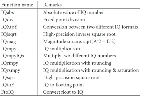
A subset of IQmath functions used in this paper is pre-sented inTable 2.
Table2: List of relevant functions from IQmath library.
Function name Remarks
IQabs Absolute value of IQ number IQdiv Fixed point division
IQXtoY Conversion between two different IQ formats IQisqrt High-precision inverse square root
IQmag Magnitude square: sqrt(Aˆ2 + Bˆ2) IQmpy IQ multiplication
IQmpyIQx Multiply two different IQ numbers IQrmpy IQ multiplication with rounding
IQrsmpy IQ multiplication with rounding & saturation IQsqrt High-precision square root
IQtoF IQ to floating point FtoIQ Convert float to IQ
In order to include an IQmath function in C code the following steps must be followed:
(i) include theIQmathLib.hinclude file;
(ii) link your code with the IQmath object code library, IQmath.lib
(iii) use a correct linker command file to place “IQmath” section in program memory;
(iv) the section “IQmathTables” contains lookup tables for IQmath functions.
The C code functions from IQmath library compile into effi-cient C64x+ assembly code. The IQmath functions are im-plemented by using C64x+ specific C language extensions (intrinsics) and compiler directives to restructure the off -the-shelf C code while maintaining functional equivalence to the original code [36]. The intrinsics are built in functions that usually map to specific assembly instructions. The C64x+ in-struction such as multiplication of two 32-bit numbers to 64-bit result is utilized to have higher precision multiplication [32].
To illustrate this step, a bit-true fixed point version of functioncholdc()shown inFigure 9is ported to fixed point DSP.
The process of porting to a fixed point target starts with a bit-true fixed point model (Figure 9). The fixed point vari-ables from listing shown inFigure 9are converted to corre-sponding fixed point formats supported by IQmath library. In listing presented inFigure 10, lines (11)–(14) and (33)– (38) convert between floating point and fixed point formats. Lines (16)–(30) from listing in Figure 10are equivalent to lines (16)–(26) from listing inFigure 9. Note that fixed point multiplication and square root operations are replaced with the equivalents from IQmath library. These functions are optimized for maximum performance on target fixed point DSP architecture.
(1) void choldc(float **aa, int n, float pp[]) (2){
(3) void nrerror(char error text[]); (4) int i,j,k,ip,iq;
(5) iq28 a[M][M]; (6) iq29 p[M]; (7) iq28 sum; (8)
(9) a=imatrix(1,n,1,n); (10) p=ivector(1,n);
(11) //convert input matrix to IQ format (12) for (i=0;i<n;i++){
(13) for (j=0;j<n;j++) a[i][j]= FtoIQ28(aa[i][j]); (14) }
(15)
(16) for (i=0;i<n;i++){ (17) for (j=i;j<n;j++){
(18) for (sum=a[i][j],k=i-1;k>=0;k- -) (19) sum -= IQ28mpy(a[i][k],a[j][k]); (20) if (i==j){
(21) if (sum<=0.0)
(22) nrerror(“choldc failed”);
(23) p[i]=IQXtoIQY( IQ28sqrt(sum),28,29);
(24) }else{
(25) iq28 tmp;
(26) tmp= IQXtoIQY(p[i],29,28); (27) a[j][i]=IQ28div(sum,tmp);
(28) }
(29) }
(30) } (31)
(32) //convert back to floating point (33) for (i=0;i<n;i++){ (34) pp[i]= IQ29toF(p[i]); (35) for (j=0;j<n;j++)
(36) aa[i][j]= IQ28toF(a[i][j]); (37) }
(38) (39) (40)}
Figure10: Fixed point implementation of Cholesky decomposition algorithm in IQmath.
a few CPU cycles can be saved if the variable is in Q28 fixed point format. If all fixed point variables in the function were inQ28 fixed point format, the function would execute slightly faster since it would not be necessary to spend CPU cycles for conversion between different formats (lines (23) and (26) inFigure 10).
Usually, the implementation optimized for a target DSP must not only run on the DSP but it should also run and simulate on a work station or a PC. Since the IQmath library functions are implemented in C, it is possible to recompile and run fixed point target DSP code on a PC or workstation providing that DSP intrinsics library for the host exists.
6. RESULTS
Real-time performance of selected numerical linear algebra algorithms is compared between their implementations on
fixed point DSP and floating point DSP platforms. Imple-mentation of the numerical linear algebra algorithms on a floating point DSP target was straight forward since their original implementation was in floating point C/C++ [18]. On the other hand, in order to run on a fixed point DSP target, the numerical linear algebra algorithms described in Section 2had to be ported to fixed point arithmetic.
The flow presented in this paper significantly shrinks the time spent on algorithm conversion from a floating point to fixed point DSP target. The conversion process turns out to be at least four times faster than trial-and-error determina-tion of the fixed point formats by hand.
The simulation speed of bit-true fixed point implementa-tion in SystemC is rather slow compared to the original float-ing point C program. The SystemC simulation runs approx-imately one thousand times slower. The simulation time re-quired for the range estimation process is 5–20 times shorter than bit-true fixed point model simulation in SystemC.
Optimization for different design criteria, like through-put, chip size, memory size, or accuracy, are in general mu-tually exclusive goals and result in a complex design. We use three points to compare performance between fixed point and floating DSP platforms for running the numerical lin-ear algebra algorithms:
(i) speed which translates to number of CPU cycles re-quired to run the algorithm, and CPU frequency; (ii) code size;
(iii) accuracy.
To optimize the speed performance of the algorithms, only compiler-driven optimization is used. We wanted to pre-serve connection to the original floating point C algorithm throughout different stages of the conversion flow described in Sections 3,4, and 5. In order to keep simple mapping between the different stages of the float-to-fixed conversion flow we did not change the original algorithms. In order to maintain portability between different platforms (work sta-tion/target DSP) the algorithm implementation is kept in C/C++. Although better performance can be achieved by im-plementation of critical functions (such as square root) in assembly this was not exploited to maintain code portability. For the occasional cases where additional CPU performance is needed, additional techniques are available to improve per-formance of C/C++ applications [38].
In the following three sections each aspect will be dis-cussed separately.
The selected numerical linear algebra algorithms are im-plemented on the TMS320C6000 DSP family from Texas In-struments.
The algorithm performance in floating point was evalu-ated on TMS320C6713 (C67x CPU core) and TMS320C6727 DSPs (C67x+ CPU core). Compiler used for both cases was v5.3.0.
The performance of the numerical algebra algorithms on the fixed point DSP is evaluated on C64x+ CPU core. To evaluate algorithm performance in fixed point, we used TMS320C6455 DSP (C64x+ CPU core). Compiler used was v6.0.1.
6.1. Number of CPU cycles/speed
6.1.1. Code/compiler optimizations
Pivoting is nothing more than interchange of rows (partial pivoting) or rows and columns (full pivoting) so as to put a particularly desirable element in the diagonal position from
which the pivot is about to be selected. Pivoting operation can be separated to (1) search for pivot element, and (2) interchange rows, if needed. Search for pivot element adds a slight overhead on a DSP since conditional branch pre-vents efficient pipelining. The computational overhead of row swapping (permutation operation) is significantly re-duced on TMS320C6000 DSPs, since, interchange of rows (once the pivot element is found), is fully pipelined by the compiler.
The Gauss-Jordan algorithm requires row operations and pivoting (swapping rows) for numerical stability. The com-piler successfully pipelines row swapping loops, and scaling loops in Gauss-Jordan algorithm.
The LU factorization algorithm uses Crout’s method with partial pivoting. Crout’s algorithm solves a set of equations by arranging the equations in a certain order. Pivoting is es-sential for stability of Crout’s algorithm. In LU decomposi-tion the compiler is successfully pipelining five inner loops: loop over row elements to get the implicit scaling informa-tion, the inner loop over columns of Crout’s method, the in-ner loop in search for largest pivot element, the row inter-change loop, and pivot divide loop.
Performing the pivoting by interchange of row indexes significantly speeds up decomposition of large matrices. In case of small matrices the pivoting by interchange of row in-dexes is only slightly faster. It takes∼30 CPU cycles to inter-change two rows in 5×5 matrix which is less than 1.5% of total number of cycles required forLUdecomposition. The accuracy of decomposition is not affected by either pivoting implementation. In our implementation of LU decomposi-tion we perform pivoting by really interchanging rows.
Cholesky decomposition is extremely stable without any pivoting. Cholesky decomposition requires multiplication, division, and the square root computation. In the fixed point implementation of Cholesky decomposition the square root, division, and multiplication are replaced by IQmath C func-tions optimized for C64x+ CPU architecture. The numerical linear algebra algorithms usually contain double- or triple nested loops. The compiler is the most aggressive on in-nermost loops. The inner loop of block dot product im-plementation of Cholesky decomposition (lines (18)-(19) inFigure 10) is successfully pipelined by the compiler. The compiler extracts an impressive amount of parallelism out of the application. Optimized with the appropriate flags the inner loop is unrolled so that a multiple of 2 elements are computed at once.
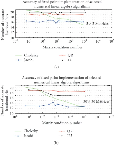
Givens and Householder transformations are frequently used in matrix factorizations [16]. When Givens rotations are used to diagonalize a matrix, the method is known as a Jacobi transformation. For this reason, Givens rotations are also known as Jacobi rotations. In numerical terms, both Givens and Housholder are very stable and accurate methods of introducing zeros to a matrix. Backward error analysis re-veals that error introduced by limited precision computation is on order of machine precision, which is an important fact given that we have limited number of bits on fixed point.
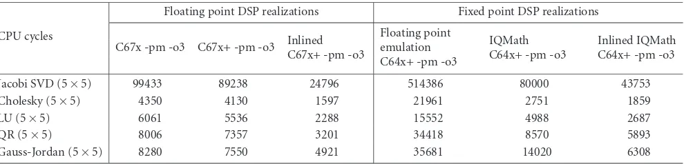
Table3: Cycle count and code size for floating point emulation of the key operations for numerical linear algebra (fixed point C64x+ CPU).
Floating point emulation on C64x+ CPU core
C64x+ [CPU clocks]
Code size [bytes]
Addition 66 384
Multiplication 69 352
Square root 3246 512
Division 114 320
when compared to most other methods, for example, QR iteration. The exact Jacobi Algorithm [16] involves the cal-culation of a square root, the calcal-culation of a reciprocal of a square root, and multiple divisions. We implement Jacobi rotations in which division, the square root computation, and the reciprocal of the square root are replaced by IQ-math C functions optimized for C64x+ CPU architecture. Algorithms to compute the Jacobi SVD are computationally intensive when compared to the traditional factorizations. Unlike Cholesky, the Jacobi SVD algorithm is iterative. We demonstrate here that Jacobi SVD algorithm translates well to fixed point DSPs; and that the convergence property of the algorithms is not jeopardized by fixed point computations. The compiler successfully pipelines four rotation loops.
In QR decomposition, we use Householder reflection al-gorithm. In practice, using Givens rotations is slightly more expensive than reflections. Givens rotations are slower but they are easier to implement and debug, and they only re-quire four temporary variables when calculating the orthog-onal operation compared with number of reflections, they are slightly more accurate than Householder method. All of these effects stem from the fact that Givens examines only two elements on the top row of a matrix at a time, whereas Householder needs to examine all the elements at once. The compiler is successfully pipelining two inner loops of succes-sive Householder transformations.
6.1.2. Target customization of critical functions
Square root, inverse square root, multiplication and divi-sion are by far the most expensive real floating point op-erations. These operations are necessary to compute Jacobi SVD, Cholesky decomposition, QR decomposition, and LU decomposition. Their efficient implementation is crucial for overall system performance. In Tables3and4, we compare performance of these functions between two implementa-tions: floating point emulation and pure fixed point imple-mentation on fixed point C64x+ CPU.Table 3presents cycle count and memory footprint when these functions are im-plemented by emulating floating point on fixed point C64x+ CPU.
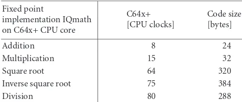
InTable 4, code size and cycle count for IQmath imple-mentation, on C64x+ CPU core, of these four critical func-tions are presented.
Table4: Cycle count and code size for IQmath implementation of the key operations for numerical linear algebra (fixed point C64x+ CPU).
Fixed point
implementation IQmath on C64x+ CPU core
C64x+ [CPU clocks]
Code size [bytes]
Addition 8 24
Multiplication 15 32
Square root 64 320
Inverse square root 75 384
Division 80 288
The IQmath division, square root, and inverse square root functions are computed using two iterations of the Newton-Raphson method. Each Newton-Raphson iteration doubles number of significant bits. First iteration gives 16-bit accuracy, and second iteration gives 32-bit accuracy. To ini-tialize the iterations a 512 byte lookup table is used for square root and inverse square root, and 1024 byte lookup table is used for division. The serial nature of Newton iterations does not allow compiler to use pipelining.
6.1.3. CPU cycle count for different algorithm realizations
InTable 5, CPU cycle counts are presented for the selected numerical linear algebra algorithms. Floating point section of Table 5 presents results for the following floating point DSP realizations:
(i) algorithm performance in CPU clocks for implemen-tation on TMS320C6711 (C67x CPU core);
(ii) algorithm performance in CPU clocks for implemen-tation on TMS320C6727 (C67x+ CPU core);
(iii) algorithm performance in CPU clocks for inline im-plementation on TMS320C6727 (C67x+ CPU core).
Fixed point section ofTable 5presents results for the follow-ing fixed point DSP realizations:
(i) algorithm performance in CPU clocks for implemen-tation using floating point emulation on C64x+ CPU core;
(ii) algorithm performance in CPU clocks for fixed point implementation using IQmath library on C64x+ CPU core;
(iii) algorithm performance in CPU clocks for fixed point implementation using inline functions from IQmath on C64x+ CPU core.
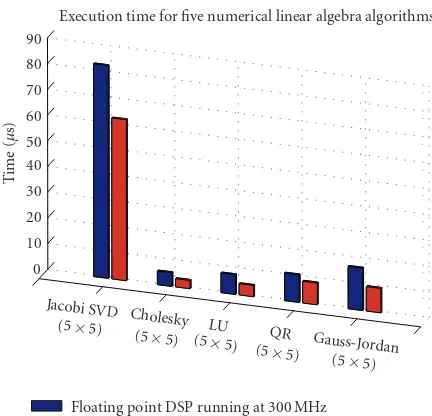
Table5: Cycle count relative to selected numerical linear algebra implementations.
CPU cycles
Floating point DSP realizations Fixed point DSP realizations
C67x -pm -o3 C67x+ -pm -o3 Inlined C67x+ -pm -o3
Floating point emulation C64x+ -pm -o3
IQMath C64x+ -pm -o3
Inlined IQMath C64x+ -pm -o3
Jacobi SVD (5×5) 99433 89238 24796 514386 80000 43753
Cholesky (5×5) 4350 4130 1597 21961 2751 1859
LU (5×5) 6061 5536 2288 15552 4988 2687
QR (5×5) 8006 7357 3201 34418 8570 5893
Gauss-Jordan (5×5) 8280 7550 4921 35681 14020 6308
fixed point and floating point CPUs is close to three. Even at clock rates that are three times higher than clock rates of the floating point DSP, the performance of floating point em-ulation on fixed point DSP is still inferior. The floating point emulation performance is satisfactory only if there are no big real-time implementation restrictions. To get the maximum performance from the fixed point DSP the algorithms must be converted to fixed point arithmetic.
The range-estimation step (Section 3) is carried in or-der to create a bit-true fixed point model (Section 4). Speed performance of numerical linear algebra algorithms on fixed point DSP becomes comparable to floating point DSP only if steps outlined in Section 5are taken. The bit-true fixed point model is adapted to a fixed point DSP target by us-ing a library of C functions optimized for C64x+ architecture (Section 5).
The two leftmost columns in the “floating point realiza-tion” part ofTable 5represent cycle counts for the algorithms executed on C67x and C67x+ floating point cores. In these cases, the floating point algorithms are calling square root, inverse square root, and division functions from an external library. The middle column of the “fixed point realization” part ofTable 5represents cycle counts for the algorithms ex-ecuted on C64x+ fixed point core. In this case, the fixed point algorithms are calling fixed point implementation of square root, inverse square root, and division functions from an ex-ternal IQmath library. Note that if exex-ternal libraries are used, algorithm realization on floating point DSP takes roughly the same amount of cycles as implementation in fixed point run-ning on a fixed point DSP. Since floating point DSPs usually run at lower clock rates, the overall execution time is much shorter on fixed point DSPs.
The maximum performance can be achieved only when inline function expansion is used (Table 5). In this case, the C/C++ source code for the functions such as square root, in-verse square root, and division is inserted at the point of the call. Inline function expansion is advantageous in short func-tions for the following reasons:
(i) it saves the overhead of a function call;
(ii) once inlined, the optimizer is free to optimize the func-tion in context with the surrounding code.
Speed performance improvement was also achieved by help-ing the compiler determine memory dependencies by ushelp-ing
Table6: Jacobi SVD algorithm: number of Jacobi rotations for dif-ferent matrix sizes.
Matrix dimension Number of Jacobi rotations
5×5 40
10×10 196
15×15 536
20×20 978
25×25 1622
30×30 2532
restrict keyword. The restrict keyword is a type qualifier that may be applied to pointers, references, and arrays. Its use rep-resents a guarantee by the programmer that, within the scope of the pointer declaration, the object pointed to can be ac-cessed only by that pointer. This practice helps the compiler optimize certain sections of code because aliasing informa-tion can be more easily determined.
By using the above optimization techniques and by us-ing the highest level of compiler optimizations, speed per-formance of the fixed point implementation can be up to 10 times improved over floating point emulation. By us-ing the above optimization, the fixed point implementation gets close in cycle counts to floating point DSP implementa-tion.
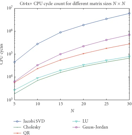
Figure 11presents number of CPU cycles required to cal-culate the selected linear algebra algorithms in fixed point arithmetic for different matrix sizesn×non a fixed point C64x+ CPU. The fixed point algorithms are implemented in pure C language, and to collect CPU cycle numbers presented inFigure 11inline function expansion and the highest com-piler optimization are used.