Initial Free Recall Data Characterized and Explained By Activation Theory of Short Term
Memory
Eugen Tarnow, Ph.D.
18-11 Radburn Road
Fair Lawn, NJ 07410
[email protected] (e-mail)
Abstract:
Introduction
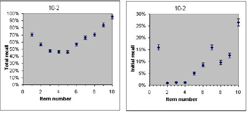
One ignored issue in short term memory research is the initial recall distribution in a free recall experiment. In Figure 1 is shown both the total recall and the initial recall in a typical ten item recall experiment (the 10-2 data from Murdock, 1962 – see Appendix 2). Both curves show the famous bowing effect (that intermediate items are remembered less well than initial or final items). Other than that, the two curves look very different. In particular, three of the items in the initial recall distribution have close to 0 recalls. There is no mention in the previous literature of this fact and there is no previous attempt to explain the initial free recall distribution.
Fig. 1. The left panel shows the famous bowed curve of total recall versus item number. The right panel shows the bowed
curve of initial recall versus item number. As a guide to the eye the error bars in each direction are the standard deviation
of a Poisson distribution (no systematic errors were considered). Experimental data from Murdock (1962).
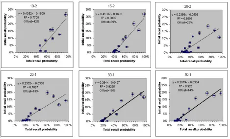
recalled in the initial recall. Figure 3 shows that the offset in each case is the same as the total recall probability of the least recalled item.
Figure 2. Number of initial recalls for each item versus the total number of recalls for that item. The six panels correspond
to the six Murdock (1962) experiments labeled on top as M-N. M is the number of items in the list and N is the number of
seconds between item presentations. Note the well defined intercepts. As a guide to the eye, the error bars in each
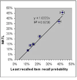
Figure 3. Offset versus recall probability of the least recalled item from the curves in Figure 3. Note the relationship
Offset=least recalled item recall probability. As a guide to the eye, the error bars in each direction are the standard
deviation of a Poisson distribution (no systematic errors were considered)
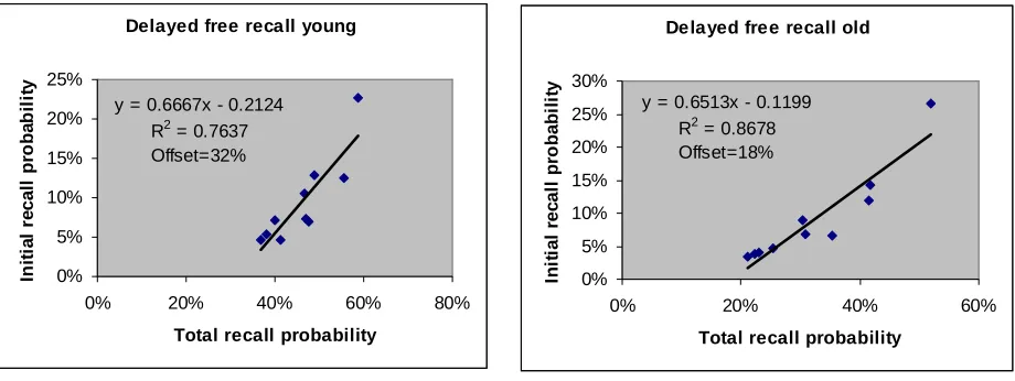
Figure 4. Number of initial recalls for each item versus the total number of recalls for that item in a delayed free recall
experiment (Kahana et al, 2002). The two panels correspond to old and young populations. For the young (old)
population the intercept is 13% (15%) lower than the probability of the least remembered item.
In this paper I will show that the initial recall distribution can be described within my activation theory of short term memory as arising from comparisons of activation levels of the presented items.
Delayed free recall young
y = 0.6667x - 0.2124 R2 = 0.7637 Offset=32% 0% 5% 10% 15% 20% 25%
0% 20% 40% 60% 80%
Total recall probability
In it ia l re c a ll p ro b a b il it y
Delayed free recall old
y = 0.6513x - 0.1199 R2 = 0.8678 Offset=18% 0% 5% 10% 15% 20% 25% 30%
0% 20% 40% 60%
Total recall probability
Activation Theory Prediction Of Initial Recall
The theory (see Appendix I) states that a short term memory is an activated long term memory (Tarnow, 2008). The activation level of a memory item is defined to be the same as the probability of recall or recognition of the item:
Activation level of item=Probability of recall or recognition of item (equation 1)
The activation level is 100% when a memory item is completely activated and subsequently decays logarithmically with time (Tarnow, 2008). For a word to be reported in a recall experiment the item has to be reactivated and the activation level has to increase back to 100%. This explains why the response time is proportional to 1-(activation level) in the high statistics data of Rubin et al (1999), see (Tarnow, 2008):
Response time=(1 – Activation level) * (Activation time)=(1-Probability of recall/recognition) * (Activation time) (equation 2)
The u-shape of the free recall curves (intermediate items are remembered less well than initial or final items) is explained by a presentation rate dependent decay (Tarnow, 2010a) – the decay is faster for higher presentation rates thus late items decay faster than initial items for which the presentation rate has not yet been established. The functional form of the decay is logarithmic in time:
Activation level = c – (Activation decay rate)*log(time) (equation 3)
elucidating the middle “asymptote” of the u-shaped curve (logarithmic decay quickly becomes slow so there is little difference between the activation levels of the middle items).
recall would look different from the overall probability of recalling that item. The single item with the lowest probability of being recalled would not be recalled at all and the items with the highest probability of recall would be more likely to be recalled than in the overall distribution. If the reactivation mechanism probes all items at the same time, the item with the highest activation level would be the one recalled – all other items would not be recalled. If n items are being reactivated at the same time the outcome would be somewhere in between.
Thus activation theory provides the following prediction of the initial recall of item i:
Probability of initial recall of item i=ΣnD(n,N)*P(n,i) (equation 4)
where D(n,N) is the normalized probability distribution of the number of items being reactivated at any one time and N+1 is the average number of items being simultaneously reactivated. n=0 corresponds to a single item and n=1 corresponds to two simultaneously reactivated items, etc. N is the only unknown quantity. It should be proportional to the number of list items (the more items the more simultaneous reactivations), so for various list lengths we write N as:
N=(number of list items)*a (equation 5)
Thus our theory has only one constant that is unknown, a. We will approximate Dn with the Poisson distribution. P(n,i) is
the probability of reactivating item i when n+1 items are simultaneously reactivated. P(0,i) is the activation level of item i, i.e. the overall distribution of item probabilities. P(1,i) is the sum over all item pairs in which i is a member; the individual terms are 0 if the activation level of item i is lower than the activation level of the other item and 1 if the activation level of item i is the higher one. The following rules apply:
ΣnΣ,iDnP(n,i)=1 (exactly one item is recalled in the initial recall). (equation 6)
and
ΣiP(n,i)=1 (exactly one item is recalled if n items are reactivated at the same time) (equation 7)
Results: Initial recall distribution described by activation theory
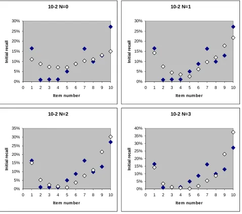
In Figure 5 is shown the activation theory prediction of the initial recall for various N for the ten item experiment in Murdock (1962). N varies from 0 (only single item reactivation) and up.
10-2 N=0 0% 5% 10% 15% 20% 25% 30%
0 1 2 3 4 5 6 7 8 9 10
Item num ber
In it ia l re c a ll 10-2 N=1 0% 5% 10% 15% 20% 25% 30%
0 1 2 3 4 5 6 7 8 9 10
Item num ber
In it ia l re c a ll 10-2 N=2 0% 5% 10% 15% 20% 25% 30% 35%
0 1 2 3 4 5 6 7 8 9 10
Item num ber
In it ia l re c a ll 10-2 N=3 0% 5% 10% 15% 20% 25% 30% 35% 40%
0 1 2 3 4 5 6 7 8 9 10
Item num ber
In it ia l re c a ll
Fig. 5. Activation theory predictions for different average number of simultaneously reactivated items N for the ten item
free recall data of Murdock (1962). The overall probability of recall for each item is the only input. As N is increased a dip
We see that as N increases, there is more of a dip in the initial recall for items that are overall the least likely to be remembered. As mentioned above, N should be proportional to the number of list items (the more items the more simultaneous reactivations), so to fit all of the Murdock (1962) data and the delayed free recall curves from Kahana et al (2002), we use a single parameter a where
a=N/(number of list items)
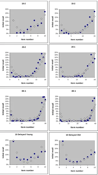
Fig. 6. Activation theory predictions of the Murdock (1962) and Kahana et al (2002) data fitted with the a parameter by
minimizing the sum of least squares. The theoretical values are shown in open diamonds and the experimental values in
filled diamonds. 10-2 0% 5% 10% 15% 20% 25% 30%
0 2 4 6 8 10
Item number In it ia l re c a ll 15-2 0% 5% 10% 15% 20% 25% 30%
0 5 10 15
Item number In it ia l re c a ll 20-2 0% 2% 4% 6% 8% 10% 12% 14% 16% 18% 20%
0 5 10 15 20
Item number In it ia l re c a ll 20-1 0% 2% 4% 6% 8% 10% 12% 14% 16% 18% 20%
0 5 10 15 20
Item number In it ia l re c a ll 30-1 0% 2% 4% 6% 8% 10% 12% 14% 16% 18% 20%
0 10 20 30
Ite m number
In it ia l re c a ll 40-1 0% 2% 4% 6% 8% 10% 12% 14% 16% 18% 20%
0 10 20 30 40
Ite m numbe r
In it ia l re c a ll
10 Delayed Young
0% 5% 10% 15% 20% 25%
0 2 4 6 8 10
Item number In it ia l re c a ll
10 Delayed Old
0% 5% 10% 15% 20% 25% 30%
0 2 4 6 8 10
Summary & Discussion
We have found that activation theory is able to explain the initial free recall distributions of the Murdock (1962) data and the Kahana (2002) data. The near zero probability of remembering lower probability items arise because comparisons between activation levels are performed and those comparisons act to amplify differences. If an item is somewhat less remembered, the first recall makes it much less remembered and if the item is the least remembered this item is almost absent from the initial recall. When something is calculated right it seems that nature rewards with excellent results. Our single parameter fit of all the initial recall distributions is such an example. The parameter, N/(number of list items)=0.14 describes the searching of our short term memory. For 7 items the average number of items reactivated at any one time is 2, for 14 items the average number of items simultaneously reactivated is 3.
APPENDIX I: The activation theory
My activation theory (Tarnow, 2008 and Tarnow, 2009, previously referred to as the Tagging/Retagging theory) started out describing the experimental data on memory decay of Rubin et al (1999) and Anderson (1981) which show a linear relationship between response time and response probability (Tarnow, 2008). The activation theory explains this linear relationship by proposing that a short term memory is an activated long term memory. When a word is heard, read from a display, or remembered, the activation level, which is the probability of recall/recognition, increases linearly in time from x% (if the item is read in for the first time x would be 0, if item is remembered x would be >0) to 100% according to equation 1:
Activation level increase = stimulus time/(Activation Time) (equation 7 – similar to equation 2)
where 0<stimulus time<Activation Time and the stimulus is either an external item read or heard or an internal item amplified during a memory search. The stimulus time is the time an item is displayed or the time an item is amplified during a search. The activation level is the probability that a word will be recalled during cued recall and the deviation of the activation level from 100% is proportional to the subjects' response time delay because the word needs to be fully reactivated. The Activation Time is related to the meaningfulness of the word – the more meaningful, the longer it takes to activate or reactivate the word. Words which lack meaning can take 0.3 seconds to activate and meaningful words can take 1.8 seconds to activate (Tarnow, 2008).
After an item is no longer displayed the activation level decreases according to equation 3 (repeated from above):
Activation level = c – (Activation decay rate)*log(time) (equation 8)
where c is a constant..
causes the word to decay from short term memory. If the endocytosis is allowed to finish (the word is not read again and is not being actively remembered), the pattern of exhausted postsynaptic terminals becomes invisible and, in our model, the short term memory of the word is gone. The long term memory remains as the pattern of the neuronal firing which is formed when a word is read.
The evidence for short term memory being related to exocytosis/endocytosis includes the shapes and slopes of the exocytosis and endocytosis curves (linear and logarithmic with time). The logarithmic decay for cued recall and recognition of words in the experiments by Rubin, Hinton and Wenzel (1999) has an associated slope of -0.11/second and endocytosis of a variety of cell ensembles in mouse hippocampus (the hippocampus is thought to play an important role in memory) varies between -0.11 and -0.14/second (Tarnow (2009) shows that experimental data, typically fitted to a sum of exponentials, is actually logarithmic). Exocytosis takes place in a quasi linear increase with a time. In one example (Dobrunz, 2002) the associated time constant (in equation 1 lagged as Activation Time) is about 1 second, similar to my finding of a activation time of 0.3-1.8 seconds for words.
In Tarnow (2010a) my activation theory explained the u-shaped free recall curve as a consequence of a presentation rate dependency of the decay of short term memory. The recency effect fits in nicely with a decay theory and the middle “asymptote”, is explained by the logarithmic time dependency which causes a large decay for the most recently activated items and a subsequently slower decay for later items. The primacy effect is explained by the dependency of the decay rate on the item presentation rate: from the data of Murdock (1962) it was found that faster presentation rates cause memory to decay faster. Since initial items have a low effective presentation rate, they decay the slowest leading to the primacy effect (typically a theory needs two variables to describe a non-monotonic curve and my activation theory uses two – the decay rate and the dependency of the decay rate on the item presentation rate).
discussion of the buffer concept see Tarnow (2010c)). In order to make this model fit the data the concepts used were contradictory and the ill-defined rehearsal concept was introduced (Tarnow, 2010b).
The experiment of Waugh and Norman (1965) is often used to argue against decay. In this experiment 16 single digits were presented at two different rates. The subjects were asked to recall the digit after the probe digit and the position of the probe digit was varied. The probability of being able to recall the subsequent digit was more sensitive to the number of digits after the probe digit than to the presentation rate, thus the authors concluded that memory does not decay with time but with interference. The result is usually plotted for 1-12 intervening items. Had the results for 13 and 14 intervening items been investigated, it would have just been shown to generate another u-shaped recall graph, not too much different from the Murdock (1962) data. Since the Murdock (1962) data can be explained with presentation rate dependent decay (Tarnow, 2010a) the Waugh & Norman data can too.
bars much too large to prove their point. The data behind the activation theory (Tarnow, 2008) shows the slow decay of short term memory on a logarithmic time scale which makes this point even harder to prove. But the main weakness of the Temporal Context Model is that it was created purely to fit the CRAP curves using abstract concepts without any regard to the underlying biology. It has lots of choices, for example, “ff one prefers the response–suppression approach, then TCM can be used to generate a set of activations, which can in turn be modulated by response suppression” (Howard & Kahana, 2001). It can be anything to anyone which also means it has no predictive power and carries no information.
Berman, Jonides and Lewis (2009) argue that interference is much more important than is decay but do not exclude decay. Here they define interference broadly: “interfering” items do not have to be similar, just tax short term memory like in the case of the counting backwards of Peterson and Peterson (1959). They state that interference “can be produced by other verbalizable items that are not similar to the to-be-remembered material.” I believe it is important to better probe this ill-defined statement: narrowing down cognitive effects to particular points in the cognitive network will tell us more about what and why interference would occur if it does. The activation theory meets these authors part of the way: it proposes that the u-shaped curve is caused by an item presentation rate dependency – the more quickly items are presented the quicker memory decays which is one way to obtain interference like effects. These authors also include a condition for decay theories: there should be a proposed process for the memory decay and the activation theory fulfills this condition.
Lewandowsky, Oberauer and Brown (2008), question decay theories on the basis of incorrect quantitative predictions of decay rates (the theories giving incorrect predictions were SIMPLE, ACT-R, PM and Trace decay). This objection does not pertain to my activation theory which is a phenomenological theory. Lewandowsky, Oberauer and Brown (2008) further argue that decay theorists can hide behind the concept of rehearsal and that rehearsal has to be carefully monitored. They state that “the notion of rehearsal is indispensable to decay models because they otherwise could not account for any persistence of immediate memory beyond a few seconds.” I argued elsewhere that rehearsal is indeed an ill-defined concept (Tarnow, 2010b) and consequently the activation theory has no rehearsal built in but it nevertheless describes the experiments of Rubin et al (1999) in which memories last a full twenty minutes.
authors also argue that the small decreases in recall at different recall speeds, or equivalent, longer delays show that there is no decay. A small decay is nevertheless a decay and can be accommodated in the activation theory, depending upon when the delay occurs and what the presentation rate is.
The Serial Order in a Box (SOB – abbreviation from model authors) interference model is a connectionist model, applied to serial recall data, in which information is stored in an associative network. The encoding strength is a function of its novelty or dissimilarity compared to what is already in the network, this being derived from the “principle that memory avoids recording redundant information” (Oberauer & Lewandowsky, 2008). But the novelty measure, is not well defined (Barrouillet and Camos, 2009). In their own words: “feature overlap,(not similarity) causes interference” (Lewandowsky, Oberauer and Brown, 2009). There is only one memory “store” in the model (Farrell, private communication) which makes it intellectually consistent but which contrasts with biochemical findings that there is a difference between short and long term memory encoding – protein synthesis is required for the latter (Kandel, 2001).
While the activation theory attempts to anchor its generalizations in biochemistry, the interference model is constructed using theoretical properties and rules that do not relate to the underlying biochemistry. These properties include “energy-gated coding”, “primacy gradient”, “response selection mechanism”, “output interference”, “response suppression”, etc (Lewandowsky and Farrell, 2008). The tests of my theory are simpler and more well defined: it can be done both via macroscopic memory experiments and microscopic biochemistry experiments.
The linear relationship between response time and response probability (Tarnow, 2008) seems to rule out interference theories in which an item is either there or it is not and there is no direct relationship between item response time and response probability. It seems that any such model would wrongly predict that the first recall distribution would be the same as the overall recall distribution. It is suggested that one such model, SOB, would account for response times in serial recall experiments (Farrell & Lewandowsky, 2004), but it has not been applied to experiments other than serial recall (Farrell, private communication).
In the activation theory the fMRI scans which apparently probe the glial cells rebuilding the neurons after firings should show a decay similar to the logarithmic time-decay discovered if this rebuilding is correlated with endocytosis.
APPENDIX II: The recall data
The Murdock (1962) data can be downloaded from the Computational Memory Lab at University of Pennsylvania (http://memory.psych.upenn.edu/DataArchive). Lists of words were read to groups of subjects to the accompaniment of a metronome (to fix the word presentation rate) after which the subjects wrote down as many of the words as they could remember in any order for a period of 1.5 minutes. There were two presentation rates: 1 or 2 seconds and there were five item list lengths – 10, 15, 20 for the two second presentation rate and 20, 30 and 40 for the one second presentation rate. The six sets of data that resulted are typically labeled M-N in which M is the number of list items and N is the number of seconds between item presentations (1 or 2).
In Kahana et al (2002) two groups of 25 subjects, one older (74 mean age) and one younger (19 mean age), studied lists of ten word items from a computer screen. Immediately following the list presentation participants were given a 16-s arithmetic distractor task and only after this delay were the subjects asked to recall the items. This data can also be downloaded from the Computational Memory Lab at University of Pennsylvania
References
Anderson JR (1981) Interference: the relationship between response latency and response accuracy. J Exp Psychol [Hum Learn] 7:326–343.
Barrouillet, P. et al. (2004) Time constraints and resource-sharing in adults’ working memory spans. J. Exp. Psychol. Gen. 133, 83–100.
Barrouillet P, Camos V (2009). Interference: unique source of forgetting in working memory? Trends in Cognitive Sciences 13(4), 145-146.
Berman MG, Jonides J, Lewis RL (2009). In search of decay in verbal short-term memory. Journal of Experimental Psychology Learning, Memory and Cognition 35 (2) 317-333.
Deese J (1959) On the prediction of occurrence of particular verbal intrusions in immediate recall. Journal of Experimental Psychology 58(1) 17-22
Dobrunz, LE. (2002) Release probability is regulated by the size of the readily releasable vesicle pool at excitatory synapses in hippocampus. : Int. J. Devl Neuroscience Vols. 20: 225-236.
Farrell S, Lewandowsky S (2004). Modelling transposition latencies: Constraints for theories of serial order memory. Journal of Memory and Language 51, 115-135.
Kahana M, Associative retrieval processes in free recall, Memory & Cognition 1996,24 (1), 103-109.
Kahana MJ, Howard MW, Zaromb F, WingField A (2002), “
Age Dissociates Recency and Lag Recency Effects in
Free Recall”
Lewandowsky S, Oberauer K, Brown G, (2009) No temporal decay in verbal short-term memory, Trends in Cognitive Sciences 13 (3) 120-126.
Lewandowsky, S., & Farrell, S. (2008). Short-term memory: New data and a model. Psychology of Learning and Motivation: Advances in Research and Theory, Vol 49, 49, 1-48.
Murdock Jr., Bennet B. (1962). The serial position effect of free recall. Journal of Experimental Psychology. Vol 64(5): 482-488.
Oberauer, K., & Lewandowsky, S. (2008). Forgetting in immediate serial recall: Decay, temporal distinctiveness, or interference? Psychological Review, 115(3), 544-576.
Peterson LR, Peterson MJ (1959) Short-term retention of individual verbal items. Journal of Experimental Psychology 58, 193-198
Rubin DC, Hinton S, Wenzel A.(1999). The Precise Time Course of Retention. Journal of Experimental Psychology: Learning, Memory and Cognition, Vols. 25:1161-1176.
Tarnow E (2008). Response probability and response time: a straight line, the Tagging/Retagging interpretation of short term memory, an operational definition of meaningfulness and short term memory time decay and search time. Cognitive Neurodynamics, 2 (4) p. 347-353.
Tarnow E (2010a) Short term memory bowing effect is consistent with presentation rate dependent decay, Cognitive Neurodynamics 2010, 4(4), 367.
Tarnow E (2010b) Why The Atkinson-Shiffrin Model Was Wrong From The Beginning, WebmedCentral NEUROLOGY 2010;1(10):WMC001021.
Tarnow E (2010c) There Is No Limited Capacity Memory Buffer in the Murdock (1962) Free Recall Data. Cognitive Neurodynamics 2010, 4(4), 395.