R E S E A R C H
Open Access
Robust adaptive filtering using recursive
weighted least squares with combined
scale and variable forgetting factors
Branko Kova
č
evi
ć
1, Zoran Banjac
2*and Ivana Kosti
ć
Kova
č
evi
ć
3Abstract
In this paper, a new adaptive robustified filter algorithm of recursive weighted least squares with combined scale and variable forgetting factors for time-varying parameters estimation in non-stationary and impulsive noise environments has been proposed. To reduce the effect of impulsive noise, whether this situation is stationary or not, the proposed adaptive robustified approach extends the concept of approximate maximum likelihood robust estimation, the so-called M robust estimation, to the estimation of both filter parameters and noise variance simultaneously. The application of variable forgetting factor, calculated adaptively with respect to the robustified prediction error criterion, provides the estimation of time-varying filter parameters under a stochastic environment with possible impulsive noise. The feasibility of the proposed approach is analysed in a system identification scenario using finite impulse response (FIR) filter applications.
Keywords:Adaptive filtering, FIR filtering, M robust parameter estimation, Recursive weighted least squares, Variable forgetting factor, Recursive variance estimation, Non-stationary noise, Impulsive noise
1 Introduction
Adaptive filtering represents a common tool in signal processing and control applications [1–6]. An overview of methods for recursive parameter estimation in adaptive filtering is given in the literature [5–7]. There is, unfortu-nately, no recursive parameter estimation that is uniformly best. Recursive least squares (RLS) algorithm has been applied commonly in adaptive filtering and system identi-fication, since it has good convergence and provides for small estimation error in stationary situations and under assumption that the underlying noise is normal [5–7]. In this context, however, two problems arise.
First, in the case of time varying parameters, forgetting factor (FF) can be used to generate only a finite memory, in order to track parameter changes [7, 8]. For a value of FF smaller than one, one can estimate the trend of non-stationarity very fast but with higher estimate variance, owing to smaller memory length. On the other hand, with a FF close to unity, the algorithm has wider
memory length and needs rather a relatively long time to estimate the unknown coefficients. However, these coefficients are estimated accurately in stationary situa-tions. Moreover, RLS with fixed value of FF (FFF) is not effective for tracking time-varying parameters with large variations. This makes it necessary to incorporate an adaptive mechanism in the estimator, resulting in the concept of variable FF (VFF). Several adaptation proce-dures have been discussed by changing the memory length of signal [7–13]. In particular, the methods re-ferred as the parallel adaptation RLS algorithm (PA-RLS) and extended prediction error RLS-based algorithm (EPE-RLS) have a good adaptability in non-stationary sit-uations [9–13]. In addition, both methods assume that the variance of interfering noise is known in advance.
The second problem arises in an application where the required filter output is contaminated by heavy tailed distributed disturbance, generating outliers [14–20]. Namely, the classical estimation algorithms optimise the sum of squared prediction errors (residuals) and, as a consequence, give the same weights to error signals, yielding a RLS type procedure. However, an adequate in-formation about the statistics of additive noise is not
* Correspondence:[email protected]
2School of Electrical and Computer Engineering, 283 Vojvode Stepe St.,
Belgrade, Serbia
Full list of author information is available at the end of the article
included in RLS computation. Possible approaches to ro-bust system identification introduce a non-linear map-ping of prediction errors. Although in the statistical literature, there are few approaches to robust parameter estimation, M robust approach (the symbol M means approximate maximum-likelihood) is emphasised, due to its simplicity for practical workers [15–23]. Robustified RLS algorithm, based on M robust principle, the so-called robustified recursive least square method (RRLS), uses the sum of weighted prediction errors as the per-formance index, where the weights are functions of pre-diction residuals [24–26]. However, M estimators provide for the solutions of the location parameters esti-mation problem [21–23]. As a consequence, in a situ-ation of non-stsitu-ationary noise signal with the time-varying variance, their efficiency should be bad [7, 24]. Therefore, a significant part of RRLS algorithm is the es-timation of unknown noise variance or the so-called scale factor [15, 16, 24, 26]. A suitable practical robust solution is the median estimator based on absolute me-dian deviations, named meme-dian of absolute meme-dian devi-ations (MAD) estimator [21–23]. However, RRLS algorithm of M robust type using MAD scale factor esti-mation is also found to be non-effective for tracking of time-varying parameters [7, 11, 24, 26]. For these rea-sons, neither of the stated algorithms alone can solve the both mentioned problems.
In this article, we design a new robust adaptive finite impulse response (FIR) system for dealing with these problems simultaneously. To alleviate the effects of non-stationary and impulsive noise, this algorithm extends the concept of M robust estimation to adaptive M ro-bust algorithm with the estimation of both filter parame-ters and unknown noise variance simultaneously. The estimated noise variance, together with the robustified extended prediction error criterion, calculated on the sliding data frame of proper length, is used to define a suitable robust discrimination function, as a normalised measure of signal non-stationarity. In addition, the VFF is introduced by the linear mapping of robust discrimin-ation function. This, in turn, enables the tacking of time-varying filter parameter under the impulsive noise. Simulation results demonstrate the effectiveness of the proposed algorithm, by the comparison with the conven-tional recursive least squares (RLS) using VFF based on the standard EPE criterion, and the adaptive M robust-based algorithm with only scale factor (RRLS).
2 Problem formulation
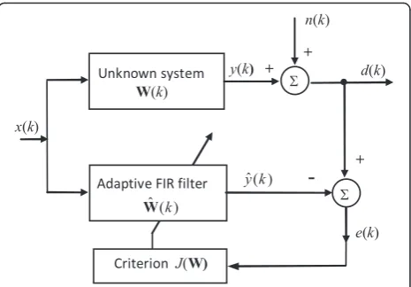
A commonly used adaptive FIR filtering scenario, expressed as a system identification problem, is pre-sented in Fig. 1. Here, x(k) is the random input signal,
d(k) is the required filter output,n(k) is the noise or dis-turbance ande(k) is the prediction error or residual. The
filter parameter vector, W(k), can be estimated recur-sively by optimising the prespecified criterion. The RLS algorithm with FF approaches the problem of estimation of non-stationary (time-varying) signal model parame-ters by minimising the sum of exponentially weighted squared residuals [5–7, 25, 26]. On the other hand, ro-bust estimates are insensitive to outliers, but are inher-ently non-linear. Moreover, most robust regression procedures are minimization problems [15–26]. Specific-ally, M robust estimates are derived as minimization of the sum of weighted residuals, instead of the quadratic performance criterion in the classical RLS computation [21–23]. To combine these two approaches, let us define a new criterion as the sum of weighted residuals
JkðW;sÞ ¼
where the prediction error (residual) signal is given by
e ið;WÞ ¼d ið Þ−XTð Þi W ð2Þ with the regression vector, X(i), and the parameter vec-tor,W, being defined by
Xð Þ ¼k ½x kð Þ; x kð −1Þ;…;x kð −nþ1ÞT; W
¼½w1;w2;⋯;wnT ð3Þ
Here, the quantities s and ρ represent the scale and forgetting factors, respectively. Moreover, W is the un-known filter parameter vector that has to be estimated. In addition, φ(⋅) is a robust score, or loss, function, which has to suppress the influence of impulsive noise, generating outliers. Having in mind the importance of reducing the influence of outliers contaminating the Gaussian noise samples, φ(⋅) should be similar to a quadratic function in the middle, but it has to increase more slowly in the tails than the quadratic one. In addition, its first derivative, ψ(⋅) =φ′(⋅), the so-called
influence function in the statistical literatures, has to be bounded and continuous [21–23, 25, 26]. The first prop-erty provides that single outlier will not have a signifi-cant influence, while the second one provides that patchy or grouped outliers will not have a big impact. A possible choice, for example, is the Huber's robust loss function, with the corresponding influence function [21].
ψð Þ ¼x min j jx
Here, sgn(⋅) is the signum function, σ is the noise standard deviation and Δ is a free parameter. This par-ameter can be adopted in such a way to provide for re-quired efficiency robustness under the zero-mean white normal noise model [21–23]. The non-linear transform-ation of data based on (4) is known in the statistical lit-erature as winsorization [21–23].
Taking the first partial derivate of (1) with respect to the elements of W in (3), say Wj,j= 1, 2,…,n, being
equal to zero, we see that the minimization of (1) re-duces to finding the solution of n non-linear algebraic relations:
where Xij is the element in the jth column of the row
vector XT(i) in (3), while ψ(⋅) is the first derivative of
φ(⋅), ψ(⋅) =φ'(⋅). Of course, for non-linear ψ(⋅), (5) must be solved by iterative numerical methods, and two suitable procedures are Newton-Raphson’s and Ditter’s algorithms, respectively, [27, 28]. Here, a slightly differ-ent approach is proposed using a weighted least-squares (WLS) approximation of (5). In this approach, the rela-tion (5) is replaced by the following approximarela-tion
Xk
i¼1
Xijβðk;iÞe ið;WÞ≈0; j¼1;2;…;n ð6Þ
where the exponentially weighted robust term is given by
βðk;iÞ ¼ρk−iωði;W0Þ ð7Þ
while its robust part is defined by
ωði;W0Þ ¼
Here,W0is an initial estimate of the parameter vector, W, which can be obtained, for example, by using the conventional non-recursive LS estimator [5, 25, 26]. The
solution of (6), say Ŵ(k), represents a one-step non-recursive suboptimal M robust estimate ofWin (3).
Application of the non-recursive M robust scheme (6)–(8) requires the non-linear residual transformation,
ψ(⋅), and scaling factor,s, to be defined in advance. But, in general, the standard deviation,σ, in (4) is not known beforehand and has to be estimated somehow. A com-monly used robust estimate of σ in the statistical litera-ture is the median scheme, based on the absolute median deviations [21–23]
s¼medianjei−medianð Þei j
0:6745 ; i¼1;2;…;L ð9Þ where L denotes the length of sliding data frame. The divisor 0.6745 in (8) is used because the MAD scale fac-tor estimate, s, is approximately equal to the noise standard deviation,σ, if the sample size,L, is large and if samples actually arise from a normal distribution [21]. Moreover, because s≈σ, Δ is usually taken to be 1.5 [21–23]. This choice will produce much better results, in comparison to the RLS method, when the corre-sponding noise probability density function (pdf ) has heavier tails than the Gaussian one. Furthermore, it will remain good efficiency of RLS when the pdf is exactly normal [21–23].
The weighting term, ω, in (8) is not strictly related to the popular robust MAD estimation of the scale factor,
s. This estimate guarantees that s≠0, but in the general case, a scale factor estimator may not guarantee that the estimate,s, should become equal to zero. This is the rea-son why the condition s= 0 is included in (8). Particu-larly, the application of a recursive robustified scale factor estimation requires the initial guess, s(0), to be given beforehand. A common choice is s(0) = 0, but in the first few steps, the obtained estimate of scale factor can be equal to zero, so that the unit value of ω in (8) has to be chosen.
the literature [12, 17–20, 29, 30]. However, similarly to sample mean and sample variance, the standard EPE ap-proach is non-robust towards outliers [21–23]. Therefore, in the next chapter, an alternative M robust approach for generating VFF adaptively is proposed.
3 A new recursive robust parameter estimation algorithm with combined scale and forgetting factors
The solution of (6) can be also represented in the com-putationally more feasible recursive form, using the well-known algebraic manipulations (for more details, see Appendix 1), [25, 26]. This results in the parameter esti-mation algorithm estimate, W0, is replaced by the preceding estimate, Ŵ(k−1), while the prediction error (residual) in (11) is given by (2), when the unknown parameter vector,W, is substituted byŴ(k−1).
Application of recursive M robust estimation algo-rithm (10)–(13) assumes the non-linear transformation,
ψ(⋅) in (4), as well as the scale factor, s in (8), and the forgetting factor,ρ in (12), to be known. Since the scale factor, s, represents an estimate of the unknown noise standard deviation, σ, and the argument of non-linearity
ψ(⋅) in (8) is the normalised residual, the non-linear transformationψ(⋅) in (8) is defined by (4) with the unit variance, i.e. σ= 1. Particularly, if one choses the linear transformation in (8), ψ(x) =x, this results in the unit weight, ω(k) = 1 in (8), and algorithm (10)–(13) reduce to the standard RLS algorithm with FF defined by (10) and (11), where the corresponding matrices, instead of (12) and (13), are given by [5, 25, 26]
In addition, if one defines the Huber’s non-linearity in (4) by using the non-normalised argument on the right-hand side of (4), yielding
ψð Þ ¼x minðj jx;ΔσÞsignð Þx ð16Þ
and approximate the first derivate,ψ′(⋅), by the weighted term ω(x) =ψ(x)/x in (8), together with the application of the winsorised residual, ψ(e), instead of original one,
e, in the parameter update equation (10), algorithm (10)–(13) can be rewritten as
where the prediction error (residual),e,is given by (11). The obtained algorithm in (3), (11), (16)–(18), repre-sents the standard M robust RLS (RRLS), where the common approach is to estimate the unknown noise standard deviation,σ, by the MAD based scale factor in (9). This algorithm can be exactly derived by applying the Newton-Raphson iterative method for solving the non-linear optimization problem in (1), with the unit pa-rameterssand ρ, respectively. Here, the non-linearity,ψ, in (16) represents the first derivative of the loss function,
φ, in (1) [24–26]. It should be noted that the parameter update equation in (17) is non-linear, in contrast to the linear parameter update equation in (10). However, both procedures for generating the weighting matrix se-quences, P(k), in (12), (13), and (18), respectively, are non-linear. Later, it will be shown that the scheme for generating the weighting matrix is very important for achieving the practical robustness.
The proposed parameter estimation algorithm (10)–(13) are derived from the M robust concept that is conservative, so the quality of parameter estimates may degrade without further adaptations ofsandρvariables.
3.1 Adaptive robustified estimation of scale factor As an adaptive robust alternative to the non-recursive robust MAD estimate in (9), the scale factor, s, can be estimated simultaneously with the filter parameter vec-tor,W. Namely, ifp nð Þis the pdf of zero-mean Gaussian white noise, n(k), in Fig. 1, with the unit variance, then the pdf of noise with some variance,σ2, is given by p nð Þ
¼p nð =σÞ=σ. Thus, one can define an auxiliary perform-ance index, in the form of the conditional maximum-likelihood (ML) criterion, [25, 26].
one can use the Newton’s stochastic algorithm for recur-sive minimization of the performance index in (19) [25, 26]. time instantk, ofW and σ, respectively. In addition, let us introduce the empirical approximation of the criter-ion (19) as
Under certain conditions, with kincreasing, Jk in (21)
approaches toJ in (19). Moreover, since p nð Þ ¼p nð =σÞ=
In addition, with large k and by using the optimality conditions, yielding
one obtains from (20)–(23) an approximate optimal so-lution in the recursive form
ks kð Þ ¼ðk−1Þs kð −1Þ
þe k ;W^ðk−1Þg e k ;W^ðk−1Þ=s kð −1Þ
ð24Þ
or equivalently
ks2ð Þ ¼k ðk−1Þs2ðk−1Þ þe2k;W^ðk−1Þωð Þk ð25Þ Here, the robust weighting term, ω(k), is defined by (8), whenψfunction is changed bygfunction, whileW0 is substituted byŴ(k−1) ands bys(k−1), respectively. As mentioned before, in M robust estimation, we wish to design estimators that are not only quite efficient in the situations when the underlying noise pdf is normal but also remain high efficiency in situations when this pdf possesses longer tails than the normal one, generating the outliers [21–27]. Thus, we can define M robust esti-mator not exactly as the ML estiesti-mator based on the stand-ard normal pdf p nð Þ, with zero-mean and unit variance, but ML estimator corresponding to a pdf p nð Þ that is similar to the standard Gaussian pdf in the middle, but has heavier tails than the normal one. This corresponds, for example, to the double exponential, or the Laplace pdf. Such choice corresponds further to the f(⋅) function in (22) being equal to the Huber’s M robust score function,
φ(⋅), in (1), with the first derivative,ψ(⋅) =φ' (⋅), given by
(4), [21–23]. Thus, in this case,g(⋅) =f' (⋅) reduces to the
ψ-function in (4), for which the noise standard deviation,
σ, is equal to one. In addition,ω(k) in (25) is given by (8), withW0and s being equal to Ŵ(k−1) and s(k−1), re-spectively. Furthermore, when the pdf,p nð Þ, is the
stand-ard normal, the influence function g(⋅) is linear and the weighting term ω(k) in (25) becomes equal to one [13]. Finally, the application of the recursive algorithm (24) or (25) requires the initial guesss(0) to be given beforehand, as it is done in Eq. (37).
The net effect is to decrease the consequence of large errors, named outliers. The estimator is then called ro-bust. In algorithm (24) or (25), this goal is achieved through the weighting term in (8), whereψis the satur-ation type non-linearity in (4). Thus, the functionψ(⋅) is linear for small and moderate arguments, but increases more slowly than the liner one for large arguments. Fur-thermore, in the normal case without outliers, one should want most of the arguments of the ψ(⋅) function to satisfy the inequality |e(i,W0)|≤Δs, because then
ψ(e(i,W0)/s) =e(i,W0)/s and ω in (8) is equal to unity. On the other hand, for large arguments satisfying |e(i, W0)| >Δs, the weighting term in (8) decreases monoton-ously with the argument absolute value and, as a conse-quence, reduces the influence of outliers.
For the scale estimation problem in question, the un-known noise variance is assumed to be constant. There-fore, after time increases, the derived recursive estimates (24) or (25) converge towards the constant value. Equa-tions (24) and (25) represent the linear combination of the previous estimate and the robustly weighted current estimation error. The coefficients in the linear combin-ation, 1−1/kand 1/k, depend on the time step,k. Thus, as kincreases, these coefficients converge towards unity and zero, respectively. As a consequence, after a suffi-ciently large time step,k, the correcting term in (24) and (25) that is multiplied by the coefficient 1/k is close to zero, so that the proposed algorithm eliminates the ef-fect of possible outliers.
Moreover, in many practical problems, it is of interest to consider the situation in which the noise variance is time-varying. However, due to the described saturation effect, the proposed estimator cannot catch the changes. These situations can be covered by simple extension of Eqs. (24) and (25). A simple but efficient solution can be obtained by resetting. The forgetting or discounting fac-tor, 1/k, in (24) and (25) is then periodically reset to the unit value, for example each 100 steps, and the initial guess,s(0), has to be set to the previous estimate.
3.2 Strategy for choosing adaptive robustifying variable forgetting factor
more heavily weights to the current samples, in order to provide for tracking of time-varying filter parameters. If a value of FF,ρ, is close to one, it needs rather long time to find the true coefficients. However, the parameter es-timates should be with high quality in stationary situa-tions. The speed of adaptation can be controlled by the asymptotic memory length, defined by [7, 25].
N¼ 1
1−ρ ð26Þ
Thus, it follows from (26) that progressively smaller values of FF, ρ, provides an estimation procedure with smaller size of data window, what is useful in non-stationary applications.
If a signal is synthetised of sub-signals having different lengths of memory, changing between a minimum value,
Nmin, and a maximum one,Nmax, the time-varying signal model coefficients can be estimated by using Eqs. (4), (8), (10–13), and (25), assigning to each sub-signal the corresponding FF, ρ, from (26), varying between ρmin and ρmax. However, in practice, the memory length and the starting points of sub-signals are unknown in ad-vance. Thus, one has to find the degree of signal non-stationarity, in order to generate the value of FF, ρ, in the next step. Although many adaptation procedures have been analysed by changing the memory length, the method using the extended prediction error (EPE) criter-ion is emphasised, since it involves rather easy computa-tion, and has good adaptability in non-stationary situations, and a low variance in the stationary one [10, 12, 13]. Particularly, the extended prediction error criter-ion, as a local measure of signal non-stationarity, is defined by [10]: Here, e(⋅) is the prediction error, or residual, in (11), and the length of the sliding window Lis a free param-eter, which has to be set.
Thus, the quantityE(k) in (27) represents a measure of the local variance of prediction residuals at the given sliding data frame of sizeL, and it contains the informa-tion about the degree of data non-stainforma-tionarity. In addition, L should be a small number compared to the minimum asymptotic memory length, so that averaging does not obscure the non-stationarity of signal. Thus, the value ofLrepresents the trade-off between the esti-mation accuracy and tracking ability of time varying pa-rameters. Unfortunately, the EPE statistics in (27), like the sample mean and sample variance, lacks robustness towards outliers [21–23]. Therefore, we suggest to derive a robust alternative to the EPE criterion in (27) using the M robust approach. Thus, if the prediction errors
e(k) in (2) are assumed to be independent and identically distributed (i.i.d) random variables, a simple parameter estimation problem can be constructed. Define a ran-dom variable (r.v.), ζ, on the sample space Ω, from which the data e(k), k= 1, 2,⋯,N, are obtained. Based on empirical measurements, the mean,me, and variance, σ2 mating Eq. (28) is non-linear, and some form of WLS approximation, similar to (6), can be used for its solu-tion. Moreover, a popular statisticsis the MAD estima-tion in (9). Althoughsin (9) is robust, it turns out to be less efficient than some other robust estimates of vari-ance [21–23]. However,sis a nuisance parameter in the computation of me, and in this context, the efficient
issue is not as crucial as in the estimation of the variance of the data, estimates of the latter being used in robusti-fying the EPE criterion (27) and setting the VFF. A more efficient estimator of the data variance should be based on the asymptotic variance formula for the location M estimate in (28). When s=σe, this formula
A natural estimate of V in (29) is
^
where VN^ in (30) would appear to be a reasonable esti-mate of σ2
e, with m^eð ÞN being the M estimate of mein
Erð Þ ¼k s2ð Þk than the criterion (31) reduces to the standard EPE cri-terion in (27), under the assumption that the scale factor estimate,s(i),i=k−L+ 1,⋯,k, on the sliding data frame of lengthLis close to thes(k) value.
On the other hand, the total noise variance robust esti-mate in (25) is rather insensitive to the local non-stationary effects. Therefore, in order to make the esti-mation procedure invariant to the noise level, one can define the normalised robust measure of non-stationarity or the so-called robust discrimination function
Q kð Þ ¼Erð Þk
s2ð Þk ð32Þ
A strategy for choosing the VFF at current time in-stant,k, may now be defined by using the relations (25), (26), (31) and (32), that is
ρð Þ ¼k 1− 1
N kð Þ; N kð Þ ¼ Nmax
Q kð Þ ð33Þ
Thus, the maximum asymptotic length, Nmax, will de-termine the adaptation speed. Furthermore, for a sta-tionary signal with possible outliers, the quantityEr(k) in
(31) will converge to the noise variance, yieldingQ(k)≈1 and N(k) =Nmax. Finally, since (33) does not guarantee
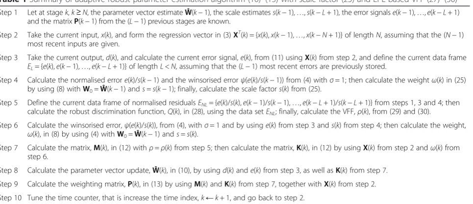
that FF,ρ, does not become negative, a reasonable limit has to be placed on FF,ρ, yielding A brief description of the proposed algorithm with both scale and forgetting factors is given in Table 1. Since the proposed algorithm combines the three adap-tive procedures (recursive robust parameter estimation, recursive robustified noise variance estimation and adap-tive robustified variable forgetting factor calculation), the theoretical performance analysis is very difficult with the coupled algorithms. Therefore, the figure of merit of the proposed approach will be given by simulations in the next section. The following algorithms are tested:
1. Recursive robust weighted least squares type method, defined by (4), (8) and (10)–(13) together with the both recursive robust scale estimation in (25) and adaptive robustified VFF calculation in (31)–(34), denoted as RRWLSV (see Table1). 2. Recursive least squares algorithm with exponentially
weighted residuals defined by (11), (14) and (15) and VFF given by (27) and (32)–(34), denoted as RLSVF. 3. Recursive robustified least squares algorithm defined by (16)–(18) and MAD-based scale factor estimation in (9), denoted as RRLSS.
4 Experimental analysis
To analyse the performances of previously discussed methods, a linear parameter estimation scenario in stationary and non-stationary contexts, related to the additive noise, is applied (see Fig. 1) [10]. The required
Table 1Summary of adaptive robust parameter estimation algorithm (10)–(13) with scale factor (25) and EPE-based VFF (27)–(30)
Step 1 Let at stagek,k≥N, the parameter vector estimateŴ(k−1), the scale estimatess(k−1),…,s(k−L+ 1), the error signalse(k−1),…,e(k−L+ 1) and the matrixP(k−1) from the (L−1) previous stages are known.
Step 2 Take the current input,x(k), and form the regression vector in (3)XT(k) = {x(k),x(k−1),…,x(k−N+ 1)} of lengthN, assuming that the (N−1) most recent inputs are given.
Step 3 Take the current output,d(k), and calculate the current error signal,e(k), from (11) usingX(k) from step 2, and define the current data frame
EL= {e(k),e(k−1),…,e(k−L+ 1)} of lengthL<N, assuming that the (L−1) most recent errors are previously stored.
Step 4 Calculate the normalised errore(k)/s(k−1) and the winsorised errorψ(e(k)/s(k−1)) from (4) withσ= 1; then calculate the weightω(k) in (25) by using (8) withW0=Ŵ(k−1) ands=s(k−1); finally, calculate the scale factors(k) from (25).
Step 5 Define the current data frame of normalised residualsENL= {e(k)/s(k),e(k−1)/s(k−1),…,e(k−L+ 1)/s(k−L+ 1)} from steps 1, 3 and 4; then
calculate the robust discrimination function,Q(k), in (28), using the data setENL; finally, calculate the VFF,ρ(k), from (29) and (30).
Step 6 Calculate the winsorised error,ψ(e(k)/s(k)), from (4), withσ= 1 and by usinge(k) from step 3 ands(k) from step 4; then calculate the weight,
filter output, d(k), is generated by passing the standard white Gaussian sequence, x(k), of the zero-mean and unit variance, through the FIR system of the ninth order, with the true values of parameters
W¼½0:1;0:2;0:3;0:4;0:5;0:4;0:3;0:2;0:1T ð35Þ
In addition, a zero-mean white additive noise, n(k), with corresponding variance is involved to its output. The value of variance is adopted so to give the desired signal-to-noise ratio (SNR) at the signal segment in question, before the impulsive noise component is intro-duced. Four situations regarding the additive noise are considered: stationary context with fixed variance and possible outliers and non-stationary context with chan-ging variance and possible outliers. The variances are chosen so to give the different values of SNR equal to 15, 20 and 25 dB, respectively. The outliers, generated by the impulsive noise, are produced using the model
n(k) =α(k)A(k), with α(k) being an i.i.d binary sequence defined by the corresponding probabilities P(α(k) = 0) = 0.99 and P(α(k) = 1) = 0.01, respectively, and A(k) is the zero-mean normal random variable with the variance var{A(k)} = 104/12 that is independent of the random variable α(k). The random variable n(k) has zero-mean and variance proportional to var{A(k)} (see Appendix 3).
A priory information of the impulsive noise is used to choose the length,L= 5, of the sliding window that cap-ture the non-stationarity. This means that no more than one outlier, in average, is in the sliding data frame of size
L= 5 during the robustified EPE calculation in (31) and MAD calculation in (9), respectively, when the fraction of outliers is 1 %.
The following algorithms, described in previous section, are tested: (1) the proposed adaptive robust filtering algo-rithm with the both robust adaptive scale and VFF, de-noted as RRWLSV; (2) the conventional RLS with EPE based VFF, denoted as RLSVF; and (3) the standard M ro-bust RLS with MAD-based scale factor, denoted as RRLS.
The analysed algorithms have been tested on both the time-varying parameter tracking ability and the log nor-malised estimation error norm
NEEð Þ ¼k 10 logk⌢Wð Þ−k Wk
2
W
k k2 ð36Þ
where ‖⋅‖ is the Euclidian norm, averaged on 30 inde-pendent runs. In each experiment, the following values are used to the initial conditions of analysed algorithms:
⌢Wð Þ ¼0 0;Pð Þ ¼0 100I; sð Þ ¼0 1 ð37Þ with I being the identity matrix of corresponding order.
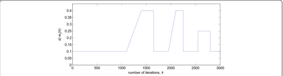
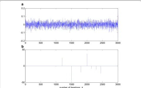
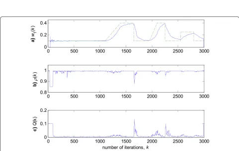
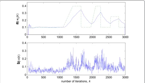
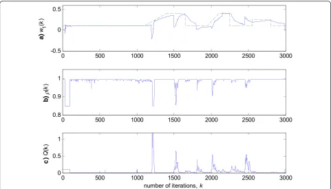
4.1 Time-varying parameter tracking in a stationary zero-mean white normal noise with possible outliers In this experiment, the first filter parameter w1in (3) is changed using the trajectory depicted in Fig. 2. The vari-ance of noise, n(k), is taken so that the SNR of 25 dB is achieved before the impulsive noise component is added. Figure 3 gives a realisation of the zero-mean white Gaussian sequence without (Fig. 3a) and with impulsive component (Fig. 3b), respectively. In Figs. 4, 5 and 6, the true and the estimated trajectories of changing param-eter, under the pure zero-mean white Gaussian noise, are shown. Moreover, the estimated scale and variable forgetting factors are also depicted in these figures. Fig-ures 7, 8 and 9 give the simulation results in the case of zero-mean and white and Gaussian noise with outliers. Figures 10 and 11 depicted the normalised estimation error in (36) obtained in the two discussed stationary noise environments, for the three analysed algorithms.
The obtained results have shown that the algorithms RRWLSV and RLSVF provide good and comparable re-sults, due to the application of VFF in the weighted matrix update equation (see Eqs. 10, 12, 14 and 15), while the algorithm RRLSS gives bad parameter tracking performance, since it uses the fixed unit value of FF in
(18), (see Figs. 4, 5, 6 and 10). Moreover, the results of simulations have indicated that the conventional RLS with VFF (RLSVF) is highly sensitive to outliers, since it does not use a robust influence function, ψ, in the par-ameter and weighted matrix update equations (see Eqs. 14 and 15). On the other hand, the RRLSS algorithm using scale factor estimation in (9), or com-bined the adaptive robustified scale and VFF factors (RRWLSV), are rather insensitive to outliers, due to the effect of robust influence function, ψ, in the parameter and weighted matrix update equations (Eqs. 17 and 18 or Eqs. 12 and 13). In addition, the algorithm RRWLSV has much better parameter tracking ability in the case of both time-varying parameters and impulsive noise envir-onment than the algorithm RRLSS (see Figs. 7, 8, 9 and 11), due to the combined effects of scale factor and VFF (see Eqs. 12 and 13).
4.2 Time-invariant parameter tracking in a non-stationary zero-mean normal noise with possible outliers
In this experiment, the filter parameters are taken to be time invariant, but the noise variance is changed during the simulation, producing a non-stationary signal. The variance of additive noise, n(k), is taken so that for the three sequential signal segments, the SNRs of 25, 15 and
20 dB, respectively, are produced, before the impulsive noise component is added. In order to obtain better cap-ture of long-term non-stationarity, in the sense of achieving good estimates of noise level changes, the scale factor,s, is averaged on the data frame of 400 sam-ples. On the other hand, this will not affect the ability of VFF algorithm to track the filter parameter changes. Figure 12 shows a realisation of noise, without (Fig. 12a) and with (Fig. 12b) impulsive noise component.
Figures 13 and 14 depict the obtained values of nor-malised estimation error (NEE) criterion in (36), without (Fig. 13) and with (Fig. 14) the presence of impulsive noise component.
In a pure zero-mean normal white noise environ-ment (see, Fig. 12a), at the beginning of parameter esti-mation trajectory, all three discussed methods have similar behaviour (Fig. 13). Moreover, all three algo-rithms are rather insensitive to the changes of noise variance, due to the effects of scale factor estimations in (9) or (25), or VFF in (27)–(34) or (31)–(34), re-spectively, and give similar results at the whole param-eter estimation trajectory, since there are no outliers (Fig. 13). The presented results in Fig. 14 indicated that the conventional RLS method with VFF (RLSVF) is highly sensitive to outliers, due to the lack of
non-a
b
Fig. 5Experimental results for RLSVF algorithm in zero-mean Gaussian noise (Fig. 3a).aEstimated (solid line) and true parameter (dashed line) trajectories (see Fig. 2).bVFF calculation,ρ(k).cDiscrimination function calculation,Q(k)
Fig. 6Experimental results for RRLSS algorithm in zero-mean Gaussian noise (Fig. 3a).aEstimated (solid line) and true parameter (dashed line) trajectories (Fig. 2).bScale factor estimation,s(k)
Fig. 8Experimental results for RLSVF algorithm in zero-mean Gaussian noise contaminated by outliers (Fig. 3b).aEstimated (solid line) and true parameter (dashed line) trajectories (Fig. 2).bVFF calculation,ρ(k).cDiscrimination function calculation,Q(k)
linear residual transformation, ψ (see Eqs. 14 and 15). On the other hand, the robust algorithms RRLSS and RRWLSV are rather insensitive to impulsive noise component, and give also comparable results, due to the effect of robust influence function, ψ, in the par-ameter and matrix update equations (see Eqs. 17 and 18 or Eqs. 12 and 13).
4.3 Time-varying parameter tracking in a non-stationary zero-mean normal noise with possible outliers
In this experiment, the simulation scenario is the com-bination of the previous two examples, with the excep-tion that the first filter parameter, w1, is adopted to be time-varying, using the parameters trajectory presented in Figs. 15, 16 and 17 depict the obtainedNEEcriterion Fig. 10Normalised estimation errorsNEEin (36), for different algorithms, in stationary zero-mean white normal Gaussian noise (SNR = 25dB); Experimental conditions are given in Figs. 2 and Fig 3a
(36), for different algorithms, without (Fig. 16) and with (Fig. 17) outliers, added to the non-stationary zero-mean normal noise with changing variance (see Fig. 12). The obtained results are in accordance to the conclusions derived from the previous two experiments.
In summary, the obtained results from the all three ex-periments have shown that, in order to properly estimate the time-varying parameters under the non-stationary and impulsive noise environment, both robustified VFF and adaptive M robust estimator with simultaneous estimation
of parameters and scale factor (RRWLSV) are required. Moreover, an adequate non-linear residual transformation in the parameter update equation (Eq. 17 in RRLSS algo-rithm) is not sufficient for protecting well against the in-fluence of outliers. Additionally, an important problem is also related to the way of recursive generation of the weighted matrix,P. It is found that the introduction of the Huber’s saturation type non-linearity,ψ, coupled with the proper decrease of the weighted matrix,P, depending on the non-linearly transformed residuals and VFF (Eqs. 12 Fig. 12Realisation of additive noise,n(k).aNon-stationary zero-mean white normal noise samples with changing variances (SNR = 25, 15 and 20 dB).
bNon-stationary zero-mean white normal noise samples, with changing variances, contaminated by outliers
and 13) provides low sensitivity to outliers and good par-ameter tracking performance (Figs. 4 and 7). The conven-tional M robust estimator (RRLSS) may converge very slowly, due to the introduction of the non-linearity first derivate,ψ′, and the unit FF in the recursive generation of the weighted matrix (Eq. 18). Namely, large residual rea-lisations, e, make the decrease of the weighted matrix,P, very slow, sinceψ′(e) = 0 in the saturation range (Eq. 18). This, in turn, results in an effect producing a slow conver-gence of parameter estimates (Figs. 6 and 9). The conven-tional RLS is also sensitive to outliers, but in a different way. In this algorithm, the weighted matrix,P, is not influ-enced by the residuals (Eq. 15). As a consequence, the fast decrease ofP, independent of residuals, leads to the biased parameter estimates in the presence of outliers (see Fig. 8).
In addition, the estimation of unknown noise variance (Eqs. 9 or 25) is essential to residual normalisation, in order to achieve a low sensitivity to the parameters defin-ing the non-linear transformation of the prediction resid-uals in (4).
4.4 Influence of outlier statistics
A real outlier statistics is not exactly known in practice, so a low sensitivity to outliers is very important for achieving the practical robustness. The effect of desensi-tising the parameter estimates related to the influence of outliers is illustrated in Tables 2 and 3, depicting the evaluation of sample mean and sample variance of the NEE statistics (36), for different outlier probability and intensity. It can be observed that the proposed algorithm Fig. 14Normalised estimation error normNEE, for different algorithms in non-stationary and impulsive noise environment (Fig. 12b), and fixed parameters in (35)
automatically damp out the effects of outliers, and it is rather insensitive to various fractions of outliers (see Table 2), up to 15 %, as well as to high level outliers (see Table 3). For higher percentage of outliers, more than 20 %, the normal noise model contaminated by outliers is not adequate. Furthermore, s(k) is a nuis-ance parameter in the estimation of filter coefficients, as well as in the VFF computation. Its proper estimate is crucial for good performance of overall estimator, consisting of three coupled adaptive schemes. Since
the complete algorithm performs quite well, this means that the estimation of scale factor also performs properly.
4.5 Influence of initial conditions
The proposed RRWLSV algorithm, exposed in Table 1, is non-linear and, consequently, may be highly influ-enced by the initial conditions, W(0) and P(0) in (33), respectively. However, from the practical point of view, a low sensitivity to the initial conditions represents the Fig. 16Normalised estimation error norm (NEE), for different algorithms, in non-stationary zero-mean Gaussian noise environment (Fig. 12a) and the time-varying parameter trajectory (Fig. 15)
desirable performance measure. Table 4 illustrates the influence of the initial condition P(0) to the estimation error.
In general, large residual realisations in the initial steps, caused by large ‖P(0)‖, can make the decrease of
‖P(i)‖ very slow. This, in turn, may result in an unde-sirable effect producing a slow convergence of filter par-ameter estimates. However, the proposed RRWLSV algorithm is found to be relatively insensitive to the ini-tial conditions, due to the proper way of generating of the weighting matrix, P(i), in (12) and (13), where the weighted term, ω(i) in (8), is used. This factor keeps the norm ‖P(i)‖ at values enough high for obtaining good convergence and, at the same time, enough small for preventing the described undesirable convergence effect. Similarly as in the experiment 4.1, it is observed that for higher values of ‖P(0)‖, the RRLSS algorithm converges very slowly. The reason lies in the introduction of the first derivative,ψ′, instead of the weighted termωin (8), in the weighted matrix update equation, P(i), in (18), which is equal to zero in the saturation range. Thus, large residuals in the initial steps, caused by large‖P(0)‖, make the decrease of ‖P(i)‖very slow. This, in turn, re-sults in the described cumulative effect, producing a slow convergence of parameter estimates (see Table 4).
4.6 Influence of model order
The selection of model structure depends on the intended model application [31]. With the adopted FIR model structure, one has to select the order, n, of the parameter vector,Win (3). The model order should not be selected too low, since then, all system dynamics can-not be described properly. However, it should can-not be se-lected too high either, since the higher the model order, the most parameters need to be estimated and the higher the variance of the parameter estimates is. Thus, increasing the model order beyond the true order of the system will not add to the quality of the model. Hence,
the model order is some sort of compromise between fitting the data and model complexity [32, 33]. Figure 18 illustrates the discussion through the obtained NEE cri-terion in (36), for the experimental conditions described in 4.1, in the cases of lower (n= 7), higher (n= 12) and exact (n= 9) model order of the FIR system.
4.7 Influence of additive noise correlations
The FIR model structure does not take into account the coloured additive noise. However, in general, additive noise,n(k), may represent any kind of noise, with arbitrary colour. Such noise can be simulated by filtering a zero-mean white noise through a linear time-invariant (LTI) system [34, 35]. In this way, one can shape the fit of a time-invariant model under a stationary noise environ-ment to the frequency domain. It can be shown that, in general case, the resulting estimate is a compromise be-tween fitting the estimated constant model parameters to the true one and fitting the noise model spectrum to the prediction error spectrum [35]. In addition, the estimates can be improved by using prefilters. The analysis is based on the limit parameter value to which the parameter esti-mates converge asymptotically and corresponding limit criterion [35]. However, such an analysis is not possible on the short data sequences, whether the situation is station-ary or not. Therefore, the answer to the question concern-ing the insensitivity to noise statistics, as well as the other questions related to the practical robustness, can be obtained only by simulations. Figure 19 depicts the obtained NEE criterion in (36), with the experimen-tal conditions exposed in 4.1, but using the coloured noise with the given autocorrelation function in Fig. 20, [36]. The experimental results indicate that the proposed RRWLSV filtering algorithm copes sat-isfactorily with the coloured noise.
It should be noted that in a FIR model structure, the noise model is fixed and equal to the unit constant.
Table 2The evaluation of the mean value and variance ofNEE, for different outlier density,ε=P(α(k) = 1)
ε 0.01 0.05 0.10 0.15 0.20 0.25 0.3
NEE
Mean value −30.2529 −30.6593 −30.1427 −30.3464 −24.4299 −18.6086 −14.2801
Variance 92.9838 95.1626 111.2679 112.4948 226.8080 322.398 410.0782
Table 3The evaluation of the mean value and variance ofNEE, for different outlier intensity,σ2
e¼ varA kð Þ, where the nominal
mean value −30.8406 −30.3820 −30.4177 −30.4417 −30.3870
variance 94.2645 92.8128 94.9259 95.1020 94.6418
Table 4The evaluation of the mean square error norm,‖P(i)‖, for different initial conditions (experimental conditions are the same as in the experiment 4.1)
P(0) 102I 10I I 0.1I
Iterations
50 366.9852 36.6985 0.3670 0.3530
100 0.9492 0.4582 1.1870 1.3091
5 Conclusions
The estimation problem of time-varying adaptive FIR filter parameters in the situations characterised by non-stationary and impulsive noise environments has been discussed in the article. The posed problem is solved ef-ficiently by application of a new adaptive robust algo-rithm, including a combination of the M robust concept, extended to the estimation of both filter parameters and unknown noise variance simultaneously, and adaptive robustified variable forgetting factor. The variable forget-ting factor is determined by linear mapping of a suitably defined robust discrimination function, representing the ratio of robustified extended prediction error criterion, using M robust approach, and M robust type recursive estimate of noise variance. Since the robustified version
of extended prediction error criterion is calculated on sliding data frame of proper length, it represents a ro-bust measure of local data non-stationarity. On the other hand, the total noise variance robust recursive estimate is rather insensitive to the local non-stationarity effects, so that the adopted robust discrimination function represents a suitable normalised robust measure of the degree of signal non-stationarity. In addition, since the total noise variance, or the so-called scale factor, and variable forgetting factor are adaptively calculated with respect to the prediction errors, the proposed algorithm works properly in stationary and non-stationary situations with possible outliers. Simulation results have shown that the new method gives higher accuracies of parameter esti-mates, and ensures better parameter tracking ability, in Fig. 18Normalised estimation error norm (NEE) in (36), for the experimental conditions described in 4.1 (Figs. 2 and 3b) and the algorithm RRWLSV, in the cases of lower (n= 7), higher (n= 12) and exact (n= 9) model order
comparison to the conventional least-squares algorithm with variable forgetting factor, and the standard M robust algorithm with scale factor estimation. Moreover, the standard least-squares algorithm with variable forgetting factor is very sensitive to outliers, while the new adaptive robust method with combined scale and variable forget-ting factor, and the conventional M robust-based method, with scale factor, are rather insensitive to such a disturb-ance. However, the proposed adaptive M robust algorithm with combined scale and forgetting factors has much better parameter tracking performance than the conven-tional M robust algorithm with only scale factor. The experimental analysis has shown that the real practical ro-bustness and good tracking performances are connected with both the non-linear transformation of prediction-residuals and an adequate recursive generation of the weighted matrix, depending on the non-linearity form and variable forgetting factor. Moreover, a recursive estimation of the unknown noise variance is essential for defining properly the non-linearity form. In summary, in order to properly estimate the time-varying parameters under the non-stationary and impulsive noise, both robustified vari-able forgetting factor and simultaneous adaptive M robust estimation of system parameters and unknown noise vari-ance are required.
The proposed adaptive M robust estimators for gener-ating scale factor and variable forgetting factor are gen-eral, while the adaptive M robust parameter estimation procedure depends on assumed signal, or system, model structure. Moreover, it can be easily applied to the other commonly used signal, or system models, including AR, ARX, ARMA and ARMAX models, respectively, or even
non-linear models. Furthermore, the proposed adaptive robustified algorithm is the one that, with proper adapta-tion, can be used as a robust alternative to the conven-tional recursive least squares or Kalman filter, respectively. These applications arise in various fields, including speech processing, biomedical signal processing, image analysis, and failure detection in measurement and control.
6 Appendix 1
6.1 Derivation of relations (10)–(13). The solution of (6) is given by
^
Wð Þ ¼k R−1ð Þk X
k
i¼1
βðk;iÞXð Þi d ið Þ ð38Þ
where
βðk;iÞ ¼ρk−iωð Þi ð39Þ
with ω(i) being defined by (8) when W0 is replaced by Ŵ(k−1). Moreover,e(i,W) in (2) is defined by (11) with W=Ŵ(k−1), while the matrixRin (38) is given by
Rð Þ ¼k X
k
i¼1
βðk;iÞXð Þi XTð Þi
¼ρXk−1
i¼1
βðk−1;iÞXð Þi XTð Þi
þωð Þk Xð Þk XTð Þk ð40Þ
Rð Þ ¼k ρRðk−1Þ þωð Þk Xð Þk XTð Þk ð41Þ Furthermore, one can also write
Xk Taking into account (38), one concludes from (42)
Xk
i¼1
βðk;iÞXð Þi d ið Þ ¼ρRðk−1ÞW^ðk−1Þ
þωð Þk Xð Þk d kð Þ ð43Þ Furthermore, by calculating ρR(k−1) from (41), and replacing it into (43), one obtains
Xk
i¼1
βðk;iÞXð Þi d ið Þ ¼Rð Þ−k ωð Þk Xð Þk XTð Þk W^ðk−1Þ
þωð Þk Xð Þk d kð Þ
ð44Þ
Finally, by replacing (44) into (38), one obtains the re-lations (10) and (11) with the gain matrix
Kð Þ ¼k R−1ð Þk ωð Þk Xð Þk ð45Þ
In addition, by introducing the weighting matrixP(k) =R−1(k), it follows from (41)
Pð Þ ¼k ρP−1ðk−1Þ þωð Þk Xð Þk XTð Þk −1 ð46Þ After applying the well-known matrix inversion lemma [25, 26]
Finally, by introducing M(k) from (12), and substitut-ing (49) into (48), one obtains the relations (12) and (13), which completes the proof.
7 Appendix 2
7.1 Derivation of relations (24)–(25). Starting from (21)–(23), one can write
kJk s=W^
In the vicinity of the optimal solution, one concludes
∂J(σ/Ŵ)/∂σ= 0 in (52), from which it follows
Furthermore, by substituting (54) in (53), one obtains
∂2J
8 Appendix 3
8.1 The derivation of mean value and variance of the random variable generating the outliers
The outliers n(k) for each time step kare generated by the random variable (r.v.) n=αA, representing the func-tion of two variables, where α is the discrete binary r.v. taking the values α1= 0 with the probability p1=P{α =α1}, andα2= 1 with the probability p2=P{α=α2},p1+
p2= 1. Moreover, A is the continuous zero-mean r.v. with varianceσ2A, and it is supposed thatαandAare in-dependent. The meanE{n} can be determined directly in terms of the joint p.d.f. fα,A(α,A) without the need for
evaluating p.d.f. ofn, that is [35]
E nf g ¼EfαAg ¼
wherem2,n and mnare non-centralized moments of the
second and the first order, respectively. Similarly as be-fore, the variance can be determined as
σ2
whereεis the density or fraction of outliers.
Abbreviations
EPE:extended prediction error; FIR: finite impulse response; FF: forgetting factor; FFF: fixed value of forgetting factor; LS: least squares; M: approximate maximum-likelihood; MAD: median of absolute median deviations; ML: maximum-likelihood;n: parameter vecor order;N: memory length; NEE: normalised estimation error; PA: parallel adaptation;Q: discrimination function; RLS: recursive least squares; RLSVF: recursive least squares with variable forgetting factor; RRLS: robustified recursive least squares; RRLSS: robustified recursive least squares with scale factor;
RRWLSV: robustified recursive weighted least squares with both scale and variable forgetting factors; SNR: signal-to-noise ratio; VFF: variable forgetting factor; WLS: weighted least-squares.
Competing interests
The authors declare that they have no competing interests.
Acknowledgments
This research was supported by Serbian Ministry of Education and Science (Project TR 32038 and III 42007)
Author details
1School of Electrical Engineering, University of Belgrade, Bulevar kralja
Aleksandra 73, Belgrade, Serbia.2School of Electrical and Computer Engineering, 283 Vojvode Stepe St., Belgrade, Serbia.3Faculty of Informatics
and Computing, Singidunum University, 32 Danijelova St., Belgrade, Serbia.
Received: 6 November 2015 Accepted: 23 March 2016
References
1. JV Candy,Model-based signal processing(John Wiley, New York, 2006) 2. SW Smith,Digital signal processing: a practical guide for engineers and
scientist(Elsevier, Amsterdam, 2003)
3. SX Ding,Model based fault diagnosis techniques, design schemes, algorithms, and tools(Springer-Verlag, Berlin Heidelberg, 2008)
4. M Barkat,Signal detection and estimation(Artech House, Norwood, 2005) 5. M Verhaegen, V Verdult,Filtering and system identification, a least squares
approach(Cambridge University Press, New York, 2012) 6. S Haykin,Adaptive filter theory(Prentice Hall, Pearson, 2013) 7. B Kovačević, Z Banjac, M Milosavljević,Adaptive digital filters
(Springer-Verlag, Berlin, Heidelberg, 2013)
8. M Basseville, A Benveniste,Detection of abrupt changes in signals and dynamical systems(Springer-Verlag, Berlin, Heidelberg, 1986)
9. S Peters, DA Antoniou, A Parallel, Adaptation algorithm for recursive least squares adaptive filters in nonstationary environments. IEEE Trans Signal Process43(11), 2484–2494 (1995). doi:10.1109/78.482100
10. YS Cho, SB Kim, EJ Powers, Time-varying spectral estimation using AR models with variable forgetting factors. IEEE Trans Signal Process 39(6), 1422–1426 (1991). doi:10.1109/78.136549
11. Z. Banjac, B. Kovačević, I. KostićKovačević,Variable forgetting factor estimation in impulsive noise environment, Telecommunications Forum
(TELFOR)22nd, Belgrade, 25–27 November 2014, pp.449–452,
doi:10.1109/TELFOR.2014.7034443
12. B. Kovačević, M. Milosavljević, M. Veinović,Time-varying AR speech analysis using robust RLS algorithm with variable forgetting factor, Proceedings of the 12thIAPR International Conference on Pattern Recognition,(Jerusalem, 09–13 October 1994),vol3,pp.211-213, doi:10.1109/ICPR.1994.577162
13. G Kvaščev,Ž Đurović, B Kovačević, I KostićKovačević,Adaptive estimation of time-varying parameters in AR models with variable forgetting factor, Mediterranean Electrotechnical Conference MELECON, (Beirut, 13–16 April 2014), pp. 68–73, doi:10.1109/MELCON.2014.6820509
14. J Chambers, A Alvonitis, A Robust, Mixed norm adaptive filter algorithm. IEEE Signal Process Lett4(2), 46–48 (1997)
15. Y Zou, SC Chan, TS Ng, Robust M-estimate adaptive filtering. IEE Proceedings Vis Image Signal Process148(4), 289–294 (2001)
16. Y Zou, SC Chan, TS Ng, A recursive least M-estimate (RLM) adaptive filter for robust filtering in impulse noise. Signal Process Lett IEEE7(11), 975–991 (2000) 17. HS Kim, JS Lim, SJ Baek, KM Sung, Robust Kalman filtering with variable
forgetting factor against impulsive noise. IEICE Trans Fundam Electron Commun Comput SciE84-A(1), 363–366 (2001)
18. T Yang, JH Lee, KY Lee, KM Sung, On robust Kalman filtering with forgetting factor for sequential speech analysis. Signal Process63(2), 151–156 (1997) 19. Y.Zhou, S. C. Chan, K. L. Ho, A new variable forgetting factor QR based
recursive least M-estimate algorithm for robust adaptive filtering in impulsive noise environment, 14thEuropean Signal Processing Conference, (Florence,
4–8 September 2006), pp. 1–5 IEEE http://ieeexplore.ieee.org/stamp/stamp. jsp?tp=&arnumber=7071126&isnumber=7065146 ISSN: 2219-5491 20. ZG Zhang, SC Chan, Recursive parametric frequency/spectrum estimation
for nonstationary signals with impulsive components using variable forgetting factor. IEEE Trans Instrum Meas62(12), 3251–3264 (2013) 21. PJ Huber, EM Ronchetti,Robust statistics(John Wiley, New Jersey, 2009) 22. RR Wilcox,Introduction to robust estimation and hypothesis testing(Academic
23. WN Venables, BD Ripley,Modern applied statistics with S(Springer, Berlin Heidelberg New York, 2002)
24. Z Banjac, B Kovačević,Robust parameter and scale factor estimation in nonstationary and impulsive noise environments, in Proceedings of IEEE Conf. EUROCON, (Belgrade, 21–24. November, 2005), pp. 1546–1549. doi:10.1109/ EURCON.2005.1630261
25. L Ljung, T Soderstorm,Theory and practice of recursive identification
(MIT Press, Cambridge, 1983)
26. YZ Tsypkin,Foundations of informational theory of identification(Nauka, Moscow, 1984)
27. M Veinović, B Kovačević, M Milosavljević, Robust nonrecursive AR speech analysis. Signal Process37(2), 189–201 (1994)
28. B Kovačević, M Veinović, M Milosavljević, M Marković,Robust speech processing(Springer Verlag, Berlin, Heidelberg, 2016). in press
29. AK Kohli, A Rai, Numeric variable forgetting factor RLS algorithm for second-order Volterra filtering. Circuits Syst Signal Process32(1), 223–232 (2013) 30. K Ak, A Rai, M Patel, Variable forgetting factor LS algorithm for polynomial
channel model. ISRN Signal Process2011, Article ID 915259 (2011) 31. PPJ van den Bosch, AC van der Klauw,Modeling, identification and
simulation of dynamical systems(CRC Press, Boca Raton, 1994)
32. R Stoica, R Eykhoff, R Janssen, T Soderstrorm, Model structure selection by cross validation. Internatt J Control43, 1841–1878 (1986)
33. H Akaike, Modern development of statistical methods, inTrends and progress in system identification, ed. by Eykhoff (Pergamon Press, New York, 1981), pp. 169–184
34. L Ljung,System identification—theory for the user, 2nd edn. (PTR Prentice Hall, Upper Saddle River, 1999)
35. B Kovačević,ŽDjurović,Fundamentals of stochastic signals, systems and estimation theory: with worked examples(Springer, Verlag, Berlin, 2008) 36. M Viswanathan,Simulation of digital communication systems using Matlab,
2013. http://www.gaussianwaves.com/simulation-of-digital-communication-systems-using-matlab-ebook. Accessed 01 march 2016
Submit your manuscript to a
journal and benefi t from:
7Convenient online submission
7Rigorous peer review
7Immediate publication on acceptance
7Open access: articles freely available online 7High visibility within the fi eld
7Retaining the copyright to your article