Simultaneous Optimization of Surface Roughness And Material
Removal Rate of Aisi 202 Steel Using Particles Swam
Optimization
1
K. Srinivasulu Reddy, 2K.Krishna Mohan Reddy 3G. Janardhana Raju3
1
Department of Mechanical Engineering Sreenidhi Institute of Science and Technology, Hyderabad
2
Department of Mechanical Engineering, Acharya Nagarjuna University, Guntur
3
Department of Mechanical Engineering, Nalla Narasimha Reddy Group of Institutions, Hyderabad
Abstract. To optimize single response problems conventional Taguchi method is popular in the design of experiments.
Performance evaluation of the manufacturing process is often determined by more than one quality characteristic. In this situation, multi-characteristics response optimization is the solution to optimize multi-objective quality characteristics. Present work is aimed at simultaneous optimization of machining problem using L8 orthogonal array (OA), and metaheuristic optimization technique Particle swam optimization.To optimize machining parameters like cutting speed, depth of cut, feed and nose radius on two different performance characteristics surface roughness (Ra) and material removal rate (MRR) during dry turning of austenitic stainless steel AISI 202 with cemented carbide tipped tool. Predictions of Taguchi and PSO matches for single objective optimization and PSO predictions for multiobjective optimization are not satisfactory because of the less complexity in the problem.
Keywords:Orthogonal array, Particle swam optimization, surface roughness, material removal rate
1. INTRODUCTION
Austenitic stainless steels are two types, 200-series and 300-series. 300-series stainless steel is most widely used. But in Asian countries, 200 series stainless steels have become more common in view of rise in nickel prices. AISI 202 stainless belongs to the low nickel and high manganese stainless steel which contains below 0.25% Nickel and manganese 7.5 to 10%. AISI 202 stainless steel is known for its high temperature strength than 18-8 steel at 800℃, with good oxidation resistance. This steel is widely used in architectural decoration, guard rail, hotel facilities, shopping malls etc.
Manufacturing industries focus their attention on surface finish and dimensional accuracy. To obtain ideal cutting parameters, they depend on the information available in machining handbooks and experience of the operator to fulfil surface finish and dimensional accuracy requirements. These traditional approaches lead to inadequate surface finish and reduced productivity due to substandard use of machining capability. This leads to low product quality and high manufacturing cost [1]. Both material removal rate (MRR) and surface roughness are important performance characteristics in turning operation. Hence, there is a need to optimize the machining parameters in an efficient way to accomplish the requirements of two response characteristics by means of design of experiments and other statistical tools.
Taguchi’s experimental design is one of the efficient and proven tool in industry to design robust experimental designs at reduced cost. These designs help to minimize
experimental trials especially when the numbers of process parameters are more. But Taguchi’s DOE approach is designed to optimize only single response problems. We can’t use this technique directly to optimize multi-response problems. Majority of the researchers concentrated on optimization of single response performance characteristic with Taguchi DOE principles [2]. As the performance of product/process is often evaluated by several quality characteristics, it is required to consider multi-response optimization. Many researchers proposed various methods to solve multi-response optimization problems by converting into optimization problem of single response [3-6].
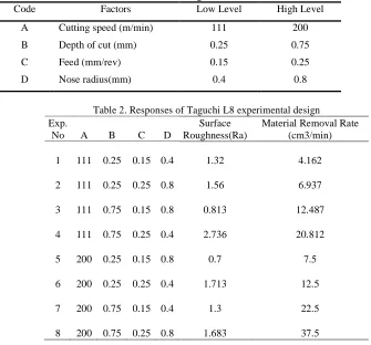
Table1. Machining Parameters and levels
Code Factors Low Level High Level
A Cutting speed (m/min) 111 200
B Depth of cut (mm) 0.25 0.75
C Feed (mm/rev) 0.15 0.25
D Nose radius(mm) 0.4 0.8
Table 2. Responses of Taguchi L8 experimental design Exp.
No A B C D
Surface Roughness(Ra)
Material Removal Rate (cm3/min)
1 111 0.25 0.15 0.4 1.32 4.162
2 111 0.25 0.25 0.8 1.56 6.937
3 111 0.75 0.15 0.8 0.813 12.487
4 111 0.75 0.25 0.4 2.736 20.812
5 200 0.25 0.15 0.8 0.7 7.5
6 200 0.25 0.25 0.4 1.713 12.5
7 200 0.75 0.15 0.4 1.3 22.5
8 200 0.75 0.25 0.8 1.683 37.5
2. METHODOLOGY
As per Taguchi’s approach responses are optimized individually, that is one response at a time.
2.1. Surface Roughness of AISI 202 Steel: Surface
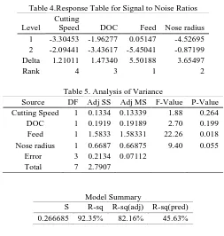
roughness of any machined component should be minimum. According to Taguchi’s methodology, smaller the better quality characteristic is to be used.Signal to Noise ratio (S/N) of surface roughness, Ra is calculated using the formula -10 log10 [Ra2]. S/N values are presented in table 3.
Following the standard Taguchi analysis, for minimum Ra, higher values of S/N ratios are obtained at A2-B1-C1-D2 settings as shown in Figure 1. Based on response table 4,feed and nose radius are more significant in achieving good surface finish. Taguchi’s predicted Ra value at A2-B1-C1-D2 settings is 0.4601 µm. Actual experimental value obtained is 1.713 µm, which is within the 95% confidence interval. ANOVA results are presented in Table 5 and corresponding regression equation is given in equation1.
Table 3. Signal to Noise ratio of Surface roughness
A B C D Ra S/N (Ra)
111 0.25 0.15 0.4 1.32 -2.41148
111 0.25 0.25 0.8 1.56 -3.86249
111 0.75 0.15 0.8 0.813 1.798189
111 0.75 0.25 0.4 2.736 -8.74232
200 0.25 0.15 0.8 0.7 3.098039
200 0.25 0.25 0.4 1.713 -4.67515
200 0.75 0.15 0.4 1.3 -2.27887
Fig 1. Main effects plot of surface roughness
Table 4.Response Table for Signal to Noise Ratios
Level
Table 5. Analysis of Variance
Source DF Adj SS Adj MS F-Value P-Value
Main Effects Plot for SN ratios
Data Means
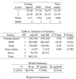
2.2 Material Removal Rate of AISI 202 steel
Material Removal Rate (MRR) should be high for any machining operation. So, larger the betterquality characteristic is chosen and Signal-to-noise(S/N) ratio is calculated using the formula, -10 log10 [1/(MRR)
2
]. S/N values calculated are presented in table 6. Main effects plot is shown in Figure 2. Based on response table 7,depth of cut and cutting speed are highly influencing material removal
rate. From standard Taguchi analysis, A2-B2-C2-D2 setting is best for high MRR with reference to high S/N values at various of process parameters and at these settings, predicted MRR is 32.21cm3/min. Actual experimental value (Exp. No.8) is 37.5 cm3/min, which is within the 95% confidence interval. ANOVA results are presented in table 8 and corresponding regression equation is presented in equation 2.
Table 6. S/N ratio of Material Removal Rate
A B C D MRR(cm3/min) S/N (MRR)
Fig.2. Main effects plot for Material removal rate 200
Main Effects Plot for SN ratios Data Means
Table 7. Response Table for Signal to Noise Ratios
Table 8. Analysis of Variance
Source DF Adj SS Adj MS F-Value P-Value local and global search combined with random search. This algorithm was originally proposed for balancing weights in neural networks, then soon later became one of the best
optimization algorithms. The popularity of PSO stems from its simplicity in performing search and especially global search since it does not need many operators for creating new solution as in evolutionary algorithms, so its implementation is straightforward [9]. But on the other hand, this algorithm suffers from two main problems: 1) slow convergence in refined search stage, and 2) Weak local search ability [10]. key concepts of PSO are given in Table 9.
Table 9. Key concepts of PSO algorithm
Concept Meaning
Swarm (X) It is the population of the algorithm which contains number of Particles.
Particle( x) Represents the potential solution as vector of M decision variables in the swarm.
pbest It is the best position of a Particle that has been achieved so far.
gbest It is the global position of the best particle in the swarm.
leader Represent the Particle that is used to guide other particles.
Velocity vector (V) It derives the optimization and determines the direction to the next move.
Inertia weight (W) It is used to control the impact of previous velocities on the current Particle’s velocity.
Learning factor (C1 and C2)
Represent the attraction of a particle to its own success or that of its neighbors.
The algorithm starts with population initialization of random solutions and velocities, and then searches for optima by updating the generations. Particles then fly through the problem space by following the current optimum Particles [39]. The position of a Particle is changed according to its own flying experience as well as the flying experience of neighbours. The pbestand gbestare updated accordingly.
2.4 Optimization of Surface roughness (Ra): Regression equation for surface roughness is given in eq.3.
z1=0.707-0.00290*x(1)+0.620*x(2)+8.9*x(3)-1.446x(4) – Eq.3
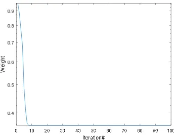
where x(1), x(2), x(3) , x(4) are cutting speed, DOC, feed and nose radius respectively. Z1 is minimised with lower bound and upper bound values as [111 0.25 0.15 0.4] and [200 0.75 0.25 0.8] respectively. From the convergence graph in Figure 3 , z1 converges to minimum after nine iterations and G.Best obtained is 0.4602 and andP.Best values are obtained at [ 200 0.25 0.15 0.8]
Fig.3 Convergence of PSO Algorithm for Ra
2.5 Optimization of MRR: Regression equation for Material
removal rate is given in eq.4
z2=-32.8+0.1*x(1)+31.1*x(2)+77.8*x(3)+2.78*x(4) –Eq.4
where x(1), x(2), x(3) , x(4) are cutting speed, DOC, feed and nose radius respectively. Z1 is minimised with lower bound and upper bound values as [111 0.25 0.15 0.4] and [200 0.75 0.25 0.8] respectively. As the algorithm is written
for minimization and the objective function has to be maximized, the regression equation for minimization of MRR is rewritten by changing the signs as given in Equation 5.
z2=32.8 - 0.1*x(1) - 31.1*x(2) -77.8*x(3) -2.78*x(4) – Eq.5
From the convergence graph in figure 4, z2 converges to minimum after nine iterations and G.Best obtained is 32.199 and andP. Best values are obtained at [ 200 0.75 0.25 0.8]
W
e
ig
h
Fig. 4. Convergence of PSO Algorithm for MRR
2.6 Multi-objective optimization of Surface roughness and Material removal rate:
Here equal weightage is given to surface roughness and material removal rate based on the customer requirements and hence w1=w2=0.5. The combined equation for optimization of both Ra (z1) and MRR(z2) is given in Equation 6.
Z= 0.5*(z1)/0.4602 – 0.5*(z2)/32.199 – Eq.6
Fig.5. Convergence of PSO Algorithm for Ra and MRR
Table 9.Comparison of different approaches
S.No Approach Response Suggested levels Predicted Values Experiment
values
1 Taguchi Ra A2-B1-C1-D2 (Exp.
No.6)
0.460125 1.713µm
2 Taguchi MRR A2-B2-C2-D2 (Exp. No. 8)
32.2188 37.5 cm3 /min
3 PSO Ra A2-B1-C1-D2 (Exp.
No.6)
0.4602µm 1.713µm
4 PSO MRR A2-B2-C2-D2 (Exp.
No.8)
32.199 cm3 /min 37.5 cm3 /min 5 PSO Ra & MRR A2-B1-C1-D2 (Exp.
No.6)
0.4602 µm and 5.759 cm3 /min
1.713 µm and 12.5 cm3 /min
3. CONCLUSIONS
For minimum surface roughness Ra, optimum levels are A2-B1-C1-D2, and value obtained experimentally is 1.713µm. For maximum material removal rate MRR, optimum levels are A2-B2-C2-D2, and experimental MRR obtained is 37.5 cm3/min. Multi-objective optimization of AISI 202 steel using Particle swarm optimization suggests A2-B1-C1-D2 experiment and predicted values of Ra is 0.4602 µm and MRR is 5.759 cm3 /min. But actual values obtained at these setting are 1.713 µm and 12.5 cm3 /min respectively.It is
observed the PSO is not effective for less complexity problems discussed here.
ACKNOWLEDGEMENTS
The authors would like to express their sincere thanks to M.Kaladharfor experimental values.
W
e
ig
h
REFERENCES
[1] Akasawa. T. Effect of free-cutting additives on the machinability of austenitic stainless steels. J. Mater. Process. Technol. 43/144, 66 (2003).
[2] Tatjana V. Sibalija, Vidosav D. Mestrovic Novel Approach to Multi Response optimization for Correlated Responses. J. of the Braz. Soc. Of Mech. Sci. & Eng. 38, 1, (2010).
[3] V. N. Gaitonde, Karnik, Paulo Davim, Multiperformance Optimization in turning of Free-machining Steel Using Taguchi Method and Utility approach. Journal of Materials Engineering and Performance,18 (3), 231 (2009).
[4] Siti AmaniahMohdChachuli , P N A Fasyar, Pareto ANOVA analysis for CMOS 0.18 micro meter two-stage Op-amp, Materials science in semiconductor processing , 24, (2014)
[5] M.Kaladhar, K.V.Subbaiah, Ch.Sreenivasa Rao, K.Narayana Rao, Application of Taguchi approach and utility approach in solving the multi-objective problem when turning AISI 202 Austenitic Stainless Steel, Journal of Engineering Science and Technology Review 4(1) 55-61, (2011)
[6] A. K. Dubey. Multi-response optimization of electro-chemical honing using utility-based Taguchi approach. Int J Adv ManufTechnol 41, 749 (2009).
[7] M.Kaladhar, Optimization of process parameter of AISI 202 austenetic stainless steel in CNC Turning. ARPN Journal of engineering and applied sciences.Vol 5, No 9, (2010)
[8] J.Kennedy, R.C Eberhart, Particle swam optimization, the 4th IEEE International conference on Neural Networks, pp.1942-1948, 1995.
[9] J.C.F Cabrera, CAC Coello, Micro MOPSO: A multi objective particle swam optimizer that uses a very small population size, Multi-objective swam intelligent Systems, Springer Berlin Heidelberg,83-104, 2010 [10] C.S. Tsou, S.C Chang, P.W.Lai using crowding distance