Automatic Image Classification for Planetary Exploration

(1)

Scholarship@Western

Electronic Thesis and Dissertation Repository

8-16-2018 11:00 AM

Automatic Image Classification for Planetary Exploration

Lei Shu

The University of Western Ontario

Supervisor

McIsaac, Kenneth

The University of Western Ontario Co-Supervisor Osinski, Gordon R.

The University of Western Ontario

Graduate Program in Electrical and Computer Engineering

A thesis submitted in partial fulfillment of the requirements for the degree in Doctor of Philosophy

Follow this and additional works at: https://ir.lib.uwo.ca/etd

Part of the Computer Engineering Commons, and the Geological Engineering Commons

Recommended Citation Recommended Citation

Shu, Lei, "Automatic Image Classification for Planetary Exploration" (2018). Electronic Thesis and Dissertation Repository. 5705.

https://ir.lib.uwo.ca/etd/5705

This Dissertation/Thesis is brought to you for free and open access by Scholarship@Western. It has been accepted for inclusion in Electronic Thesis and Dissertation Repository by an authorized administrator of

(2)

Autonomous techniques in the context of planetary exploration can maximize scientific return

and reduce the need for human involvement. This thesis work studies two main problems in

planetary exploration: rock image classification and hyperspectral image classification. Since

rock textural images are usually inhomogeneous and manually hand-crafting features is not

always reliable, we propose an unsupervised feature learning method to autonomously learn

the feature representation for rock images. The proposed feature method is flexible and can

outperform manually selected features. In order to take advantage of the unlabelled rock

im-ages, we also propose self-taught learning technique to learn the feature representation from

unlabelled rock images and then apply the features for the classification of the subclass of rock

images.

Since combining spatial information with spectral information for classifying hyperspectral

images (HSI) can dramatically improve the performance, we first propose an innovative

frame-work to automatically generate spatial-spectral features for HSI. Two unsupervised learning

methods, K-means and PCA, are utilized to learn the spatial feature bases in each decorrelated

spectral band. Then spatial-spectral features are generated by concatenating the spatial

fea-ture representations in all/principal spectral bands. In the second work for HSI classification, we propose to stack the spectral patches to reduce the spectral dimensionality and generate

2-D spectral quilts. Such quilts retain all the spectral information and can result in less

con-volutional parameters in neural networks. Two light concon-volutional neural networks are then

designed to classify the spectral quilts. As the third work for HSI classification, we propose

a combinational fully convolutional network. The network can not only take advantage of

the inherent computational efficiency of convolution at prediction time, but also perform as a collection of many paths and has an ensemble-like behavior which guarantees the robust

performance.

Keywords:autonomous techniques, planetary exploration, rock image classification,

unsuper-vised feature learning, self-taught learning, hyperspectral image classification, spatial-spectral

features, support vector machine (SVM), spectral quilts, convolutional neural network (CNN),

combinational fully convolutional network (CFCN)

(3)

Chapters 3 through 6 are co-authored with two supervisors.

Kenneth McIsaac is the student’s primary research supervisor in the graduate program in

Electrical and Computer Engineering. He provided guidance throughout the research program,

including in the selection and formulation of the problems, and selection and evaluation of

techniques to address them.

Gordon R. Osinskiis the student’s co-supervisor providing guidance especially in planetary

geology. He provided insight and instruction in the practice of terrestrial and planetary field

geology.

(4)

The thesis would not have been possible without the support of many people. I would like

to express my sincere gratitude to my supervisors, Dr. Kenneth McIsaac and Dr. Gordon

Osinski, for their continuous support, encouragement and advice. They have provided helpful

and close guidance throughout the research program and the guidance has consistently been

helpful, timely, and respectful.

Thanks as well to the team members of the research group for their kindness, valuable advice

and enlightening discussion. Special thanks to Matthew Cross and Duane Jacques for sharing

their thesis writing skills which are extremely helpful to me.

I would like also to acknowledge the funding from China Scholarship Council without which

I would not have afforded the study as an international student. Finally, I would like to thank my parents for a lifetime of uncompromising support.

(5)

Abstract i

Co-Authorship Statement ii

Acknowledgements iii

List of Figures viii

List of Tables xiii

List of Abbreviations xvi

1 Introduction 1

1.1 Planetary exploration . . . 1

1.2 Autonomous science . . . 4

1.3 Research problems . . . 5

1.3.1 Rock image classification . . . 6

1.3.2 Hyperspectral image classification . . . 7

1.4 Research contribution . . . 8

2 Literature Review and Background 11 2.1 Rock image classification . . . 11

2.1.1 Background . . . 11

2.1.2 Related work . . . 12

2.2 Hyperspectral image classification . . . 14

2.2.1 Background . . . 14

2.2.2 Related work . . . 15

(6)

2.3.2 Principal component analysis . . . 20

2.3.3 PCA-whitening . . . 21

2.3.4 Support vector machine . . . 22

2.3.5 Convolutional neural network . . . 26

2.3.5.1 Convolutional layer . . . 27

2.3.5.2 Pooling layer . . . 28

2.3.5.3 Fully-connected layer . . . 28

2.3.5.4 Regularization methods . . . 29

2.4 Summary . . . 30

3 Unsupervised Feature Learning for Autonomous Rock Image Classification 40 3.1 Introduction . . . 40

3.2 Rock image dataset . . . 42

3.3 Methods . . . 43

3.3.1 Feature representations . . . 43

3.3.1.1 Manual features . . . 43

3.3.1.2 Unsupervised feature learning based on K-means . . . 46

3.3.2 Classification method . . . 47

3.3.3 Self-taught learning . . . 48

3.4 Experimental design . . . 49

3.5 Results and Discussion . . . 51

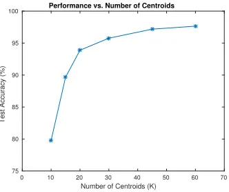
3.5.1 Parameters for unsupervised feature learning . . . 51

3.5.1.1 Number of centroids . . . 51

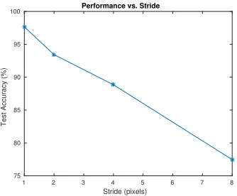
3.5.1.2 Stride . . . 52

3.5.1.3 Receptive field size . . . 52

3.5.2 Performance comparison . . . 53

3.6 Conclusion . . . 55

4 Learning Spatial-spectral Features for Hyperspectral Image Classification 59 4.1 Introduction . . . 59

(7)

4.2.1.1 Parallel computing . . . 62

4.2.1.2 Feature Extraction Approach #1: Spatial-Kmeans . . . 62

4.2.1.3 Feature Extraction Approach #2: Spatial-PCA . . . 63

4.2.2 Classifier . . . 64

4.3 Experiments and results . . . 65

4.3.1 Hyperspectral datasets . . . 65

4.3.1.1 Indian pines . . . 65

4.3.1.2 Pavia University . . . 65

4.3.2 Analysis and discussion . . . 68

4.3.2.1 Preprocessing the spectral image . . . 68

4.3.2.2 Parallel computing . . . 69

4.3.2.3 Feature bases . . . 71

4.3.2.4 Parameter sensitivity analysis . . . 71

4.3.2.5 Performance comparison . . . 74

5 Hyperspectral Image Classification with Stacking Spectral Patches and Convo-lutional Neural Networks 83 5.1 Introduction . . . 83

5.2 Method . . . 84

5.2.1 Preprocessing hypespectral data . . . 85

5.2.1.1 PCA whitening . . . 85

5.2.1.2 Stacking spectral patches . . . 86

5.2.2 Convolutional neural networks . . . 89

5.2.2.1 CNN-1 . . . 89

5.2.2.2 CNN-2 . . . 89

5.3.1.1 Indian pines . . . 90

(8)

5.3.2 Analysis of PCA whitening . . . 94

5.3.3 Analysis of patch size . . . 96

5.3.4 Performance comparison . . . 96

6 Hyperspectral Image Classification with Combinational Fully Convolutional Network 104 6.1 Introduction . . . 104

6.2 Method . . . 107

6.2.1 1×1 convolutional layers . . . 108

6.2.2 Combinational fully convolutional network . . . 108

6.3.1.1 Indian pines . . . 110

6.3.1.2 Pavia University . . . 110

6.3.1.3 Salinas scene . . . 111

6.3.1.4 Data splitting . . . 113

6.3.2 Analysis of PCA-whitening . . . 115

6.3.3 The first 1×1 convolutional layer . . . 115

6.3.4 Characteristics of CFCN . . . 119

6.3.5 Patch size . . . 120

6.3.6 Process at prediction time . . . 122

6.3.7 Computational cost and performance comparison . . . 123

6.3.7.1 Computational cost . . . 123

6.3.7.2 Performance comparison . . . 124

7 Conclusion 130

Curriculum Vitae 133

(9)

1.1 Artist’s conception of (a) MER rovers (Spirit and Opportunity) and (b) MSL

rover (Curiosity). Photo courtesy of NASA/JPL. . . 2 1.2 (a) Airborne remote sensing (b) Spaceborne remote sensing. . . 3

1.3 A hyperspectral image cube. This image was acquired in 1997 over

Mof-fett Field in California by the Airborne Visible-Infrared Imaging Spectrometer

(AVIRIS), developed by NASA JPL Laboratory. Photo courtesy of NASA. . . . 7

2.1 The typical framework of image classification. . . 13

2.2 Process and effect of PCA-whitening. (a) unwhitened data, where the two fea-tures are clearly correlated with each other. (b) rotate the data to reduce the

correlation. (c) whitened data, where features are less correlated and both have

the same variance. . . 22

2.3 SVM learns a hyperplane with the largest margin. . . 22

2.4 A typical framework of CNN. . . 27

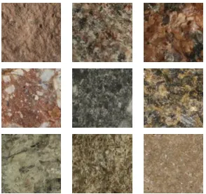
3.1 Sample images from dataset. Each sample stands for one class. All images

have size of 128×128×3 pixels and are between 1 and 2 cm across . From top

to bottom, the first column – rhyolite, volcanic breccia, limestone; the second

column – granite, andesite, oolitic limestone; the third column – red granite,

peridotite, dolostone. . . 43

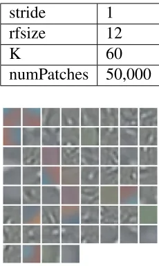
3.2 60 centroids learned from training dataset, each centroid has size of 12×12×3,

configuration of parameters refers to Table 6.1. . . 47

3.3 Framework of representing a rock image with learned features. . . 47

3.4 Framework of self-taught learning. . . 50

3.5 Dataset separation. MF-manual features, FL-feature learning, STL-self-taught

learning. . . 50

(10)

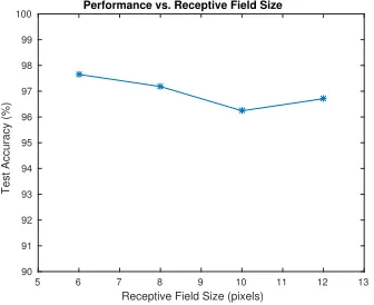
3.7 Performance vs. stride, K=60, rfsize=6. . . 52

3.8 Performance vs. receptive field size, K=60, stride=1. . . 53

4.1 Framework for generating spatial-spectral features. B is the number of spectral

bands, W is the patch size and N is the number of spectral cuboids cropped

from the spectral image. In each cuboid, the host pixel lies in the middle of the

W by W neighboring patch. . . 61

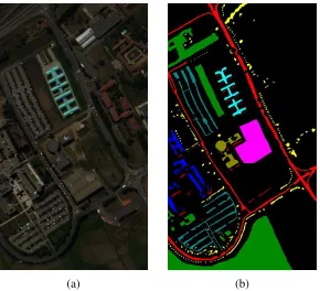
4.2 Indian Pines dataset. (a) False-color composition of bands 50, 27 and 17. (b)

Ground-truth map. The specific classes denoted by different colors refer to Table 4.1. . . 66

4.3 Pavia University scene. (a) True-color composition of bands 53, 31 and 8. (b)

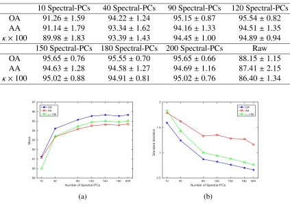
4.4 (a) Mean and (b) standard deviation of three measurements - OA, AA andκ

-over 10 random runs with different number of Spectral-PCs retained for Indian pines dataset. . . 70

4.5 Feature bases learned from Indian Pines dataset by both Spatial-Kmeans and

Spatial-PCA feature methods. The patch size is set to 15 pixels. From top to

bottom, each row corresponds to one spectral band and 5 rows correspond to

the top 5 Spectral-PCs. (a) K-means features bases - Spatial-centroids. Each

row lists 5 centroids for one certain band. (b) PCA feature bases - Spatial-PCs.

Each row lists top 5 Spatial-PCs for one certain band. . . 71

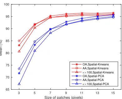
4.6 Performance with different patch size for Indian pines. Spatial-centroids/ Spatial-PCs is set to 5 and top 150 Spectral-Spatial-PCs are retained. The measurements refer

to Table 4.5. . . 72

4.7 Performance with different number of Spatial-centroids/Spatial-PCs for Indian pines. Patch size is set to 15 and top 150 Spectral-PCs are retained. . . 73

(11)

pines. Patch size is set to 15 and top 10 Spectral-PCs are retained. 20% samples

are randomly selected for training with linear-SVM. Measurements refer to

Table 4.6. . . 73

4.9 Classified maps of Indian Pines with different methods. S-Kmeans is Spatial-Kmeans and S-PCA is Spatial-PCA. . . 76

4.10 Classified maps of Pavia University with different methods. S-Kmeans is Spatial-Kmeans and S-PCA is Spatial-PCA. . . 78

5.1 Framework of hyperspectral image classification. (a) CNN-1, (b) CNN-2. . . . 85

5.2 Process and effect of PCA whitening. (a) unwhitened data, where the two features are clearly correlated with each other. (b) rotate the data to reduce the

correlation. (c) whitened data, where features are less correlated and both have

the same variance. . . 86

5.3 The benefits of stacking spectral patches. (a) three ways of convolutional

oper-ation in the first layer of CNN, namely 1) 2-D convolution with the number of

channels of convolution kernel matching the number of spectral bands, 2) 3-D

convolution with fewer channels of convolution kernel and 3) 2-D convolution

on spectral quilts. Table 5.1 shows that the proposedstacking spectral patches

has fewer convolution parameters and is computationally efficient. (b) new pat-terns (see the red squares) can be found in the spectral quilt and are effective at separating classes. . . 88

5.4 Indian Pines dataset. (a) False-color composition of bands 50, 27 and 17. (b)

5.6 Normalized pairwise correlation distribution of Indian Pines and Pavia

Univer-sity scene. . . 94

(12)

CNN-2 & Pavia University. . . 95

5.8 Performance over different patch sizes of spectral cuboid. (a) CNN-1 & Indian Pines, (b) CNN-2 & Indian Pines, (c) CNN-1 & Pavia University, (d) CNN-2

& Pavia University. . . 97

5.9 Training rate over the epochs for two networks. (a) Indian Pines, (b) Pavia

University. For both datasets, the training loss of CNN-2 converges faster than

the one of CNN-1. . . 98

6.1 The mechanism of FCN and its efficiency for predicting a map. During training, a FCN produces only one single output (top) corresponding to the central pixel

in the input patch. When applied at prediction time over a larger patch, it

produces a spatial map, e.g. 2×2 map (bottom) corresponding to the central 2×

2 pixels in the input patch. Because all layers are applied convolutionally, the

extra computation required for the lager patch is limited to the yellow regions.

This diagram omits the feature dimension for simplicity. . . 105

6.2 The architecture of the proposed family of FCNs. It consists of three 1 ×1

convolutional layers at the two ends (inside the red rectangles) and a set of

conjunct 3×3 and/or 5×5 convolutional layers in the middle (inside the green rectangle). The first 1×1 convolutional layer is used to learn overcomplete

feature maps, which in some sense increases the spectral bands of hyperspectral

images and the last two work in the same way as fully connected layers do.

Suppose we crop the 15×15 neighbor regions as the training samples for the

central pixels. There will be 21 different architectures with sets of conjunct 3×3 and/or 5×5 convolutional layers (with valid padding) to shrink the patch size from 15 down to 1. . . 108

6.3 The combinational fully convolutional network (CFCN) is the unique

combi-nation of all the 21 networks listed in Figure 6.2. . . 109

(13)

ff

Table 6.1. . . 111

6.6 Salinas scene dataset. (a) False-color composition of bands 50, 27 and 17. (b)

6.7 Normalized pairwise correlation distribution of three datasets. . . 116

6.8 Performance with/without PCA-whitening for (a) Indian Pines, (b) Pavia Uni-versity and (c) Salinas. The bars and the vertical lines on the top stand for

the average and the standard deviation of performance metrics over 10 runs,

respectively. The detailed performance refers to Table 6.5. . . 117

6.9 Analyzing the characteristic of CFCN. (a) indicates the index of each

skip-connection, (b) illustrates the predicting performance after deleting each

indi-vidual skip-connection, (c) shows the performance after deleting various

num-ber of skip-connections among the later 5 ones. . . 121

6.10 CFCN with different input patch sizes. . . 122 6.11 The whole process of predicting a map with combinational fully convolutional

network. . . 123

6.12 Loss convergence over epochs during training in Indian Pines. . . 125

6.13 Classified maps with different methods. The first row is for Indian Pines, the second row is for Pavia University and the third row is for Salinas scene.

The columns are (a) the ground-truth maps, (b) Chen2016, (c) Cao2017, (d)

Cao2017-Plus, (e) Paoletti2017, (f) SSRN, and (g) CFCN. . . 126

(14)

3.1 9 types of rocks used for classification in this study. . . 42

3.2 Parameter configuration for feature learning. stride - step size between two

adjacent sub-patches, rfsize - receptive field size, K - number of centroids,

numPatches - number of sub-patches extracted for training. . . 47

3.3 Performance of different methods. MF-manual features, FL-feature learning, STL-self-taught learning. . . 54

4.1 Classes for the Indian Pines scene and their respective number of samples. . . . 66

4.2 Classes for the Pavia University scene and their respective number of samples. . 67

4.3 Performance of different ways of preprocessing the original spectral image of Indian Pines. . . 70

4.4 Time cost of serial/parallel computing for Spatial-Kmeans and Spatial-PCA for Indian pines. . . 70

4.5 Performance with different patch size for Indian pines. Spatial-centroids/PCs is set to 5 and top 150 Spectral-PCs are retained. . . 72

4.6 Performance with different number of Spatial-centroids/Spatial-PCs for Indian pines. Patch size is set to 15 and top 10 Spectral-PCs are retained. 20% samples

are randomly selected for training with linear-SVM. . . 73

4.7 Performance comparison for Indian pines with different methods - Spectral, LADA [30], LBP [8], EMAP [3, 2], GCK [5], 3DDWT [31] and SMLR-SpATV

[32], Spatial-Kmeans and Spatial-PCA. Top 150 Spectral-PCs are retained for

both Spatial-Kmeans and Spatial-PCA. . . 75

(15)

tral, LADA [30], LBP [8], EMAP [3, 2], GCK [5], 3DDWT [31] and

SMLR-SpATV [32], Spatial-Kmeans and Spatial-PCA. All the Spectral-PCs are

re-tained for both Spatial-Kmeans and Spatial-PCA. . . 75

5.1 The number of parameters and computational complexity for three ways of

convolutional operation (with “same” padding) for one filter in the first layer

of CNN illustrated in Fig. 5.3.a. SQ is short for spectral quilts. . . 88

5.2 Architecture of CNN-1. . . 89

5.3 Architecture of CNN-2. Note that *.out stands for the output of *th layer. Two

bold layers are the shortcuts in residual blocks. . . 90

5.6 Image size after stacking spectral patches over different patch size. . . 93 5.7 Performance with PCA whitening and without PCA whitening. The patch size

is set to 15. Ouistands for with PCA whitening and Non stands for without

PCA whitening. . . 95

5.8 Performance over different patch sizes of spectral cuboid. . . 96 5.9 The number of trainable parameters in CNN-1 and CNN-2 when patch size is

set to 7. . . 97

5.10 Performance comparison with different methods - EMAP [19], GCK [20], SMLR-SpATV [21], 3DDWT [22], Chen2016 [23], Lee2017 [8], Cao2017

[24], CNN-1 and CNN-2. . . 99

6.3 Classes for Salinas scene and their respective number of samples. . . 114

6.4 Data splitting for three datasets. . . 114

6.5 Performance with/without PCA-whitening. The patch size of spectral cubes is set to 15. Yes stands for with PCA-whitening and No stands for without

PCA-whitening. . . 116

(16)

convolutional layer. Noneis the network without the 1×1 convolutional layer.

None+128is the network without 1×1 convolutional layer but increasing the

kernel sizes of the first three convolutional layers from 64 to 128. The input

patch size is set to 17 for all the networks. . . 118

6.7 Performance enhancement in Indian Pines by adding 1×1 convolutional layer

in front for Lee2017 [9] and Cao2017 [14]. *-Plus stands for the enhanced

network. Patch size is 5 for Lee2017 and 17 for Cao2017. . . 119

6.8 Predicting performance on Indian Pines after deleting each individual

skip-connection.intactstands for the full network. . . 120

6.9 Performance of CFCN over different patch sizes. . . 122 6.10 The computing resource consumption (time and memory) for different

meth-ods. Memory cost is simply the size of data ready to input to network. The

data type is npy float16.CFCN-Yesstands for the proposed network with

con-volutional implementation of sliding window at predicting time andCFCN-No

stands for the proposed network without convolutional implementation of

slid-ing window. . . 124

6.11 Performance comparison with the other state-of-the-art networks. . . 125

(17)

AA Average accuracy

AEGIS Autonomous exploration for gathering increased science

AP Attribute profile

ASTER Advanced spaceborne thermal emission and reflection radiometer CFCN Combinational fully convolutional network

CK Composite Kernel

CNN Convolutional neural network

CRISM Compact Reconnaissance Imaging Spectrometer for Mars

DBN Deep belief network

EMAP Extended multi-attribute profile EMP Extended morphological profile

ESA European Space Agency

FCN Fully convolutional network GLCM Gray level co-occurrence matrix

HSI Hyperspectral imaging

κ Kappa coefficient

MER Mars exploration rovers

MP Morphological profile

MRF Markov random field

MRO Mars Reconnaissance Orbiter

MSI Multispectral imaging

MSL Mars science laboratory

NASA National Aeronautics and Space Administration

OA Overall accuracy

OASIS Onboard autonomous science investigation system

OMEGA Observatoire pour la Min´eralogie, l’Eau, les Glaces et l’Activit´e PCA Principal component analysis

ROSIS Reflective Optics System Imaging Spectrometer RRSC Russian Roscosmos State Corporation

SSP Stacking spectral patches

SVM Support vector machine

(18)

Introduction

The present work develops new approaches to autonomous science in the context of planetary

exploration. Such missions have produced tremendous amounts of data from the instruments

they carry, requiring autonomous techniques to enhance the efficiency of scientific data analysis and enlarge the scientific returns. We address two specific problems, rock image classification

and hyperspectral image classification and produce new techniques to automatically model the

feature representation of images and conduct the classification.

1.1 Planetary exploration

The last two decades have seen unprecedented achievements in space missions on Earth and

extraterrestrial planets and we expect the scope of exploration to increase as it is powered by

human’s infinite curiosity. Take surface missions on Mars as examples. Mars Exploration

Rovers (MER) [1] and Mars Science Laboratory (MSL) [2] are two of the most successful

surface missions on Mars by NASA. MER mission (started in 2003) has two Mars rovers,

Spirit and Opportunity, exploring Martian surface and searching for and characterizing a wide

range of rocks and soils that hold clues to past water activity on Mars. MSL mission (began

in 2012) has a car-sized rover, Curiosity, investigating the Martian climate and geology, as

well as assessing the environmental conditions of the selected field site for microbial life in

(19)

preparation for human exploration. Figure 1.1 illustrates the artist’s conception of both MER

rovers and MSL rover. In the near future, Mars2020 [3] from NASA and ExoMars [4] from

ESA/RRSC are two Mars rover missions which will be launched both in 2020. Mars2020 is intended to investigate an astrobiologically relevant ancient environment on Mars and the

surface geological processes and history. ExoMars rover is to search for the existence of past

life on Mars.

(a) (b)

Figure 1.1: Artist’s conception of (a) MER rovers (Spirit and Opportunity) and (b) MSL rover (Curiosity). Photo courtesy of NASA/JPL.

In addition to the surface missions which closely explore the planet, there have been several

successful orbital missions which utilize imaging spectrometers to remotely observe the

sur-face/atmosphere of Earth/Mars without physical contact (this is also called remote sensing). The spectrometers record the electromagnetic radiation of the materials which can be used

to identify and map the materials. As indicated in Figure 1.2, there are mainly two types of

remote sensing, airborne and spaceborne remote sensing. Following are several successful

remote sensors/imaging systems.

Airborne Visible/Infrared Imaging Spectrometer (AVIRIS) [5] is an airborne hyperspectral sen-sor in the realm of Earth remote sensing. It scans the Earth’s surface and produces calibrated

images of the upwelling spectral radiance in 224 contiguous spectral bands with wavelength

range from 0.4 to 2.5 µm. The main objective of the AVIRIS project is to identify, measure,

and monitor constituents of the Earth’s surface and atmosphere based on molecular absorption

and particle scattering signatures. Research with AVIRIS data is predominantly focused on

(20)

Recon-(a) (b)

Figure 1.2: (a) Airborne remote sensing (b) Spaceborne remote sensing.

naissance Imaging Spectrometer for Mars (CRISM) [6] aboard NASA’s Mars Reconnaissance

Orbiter (MRO, launched by NASA in 2005) is a hyperspectral imaging system, operating from

3.62 to 3.92 µm wavelength with 6.55 nm per channel spacing. The best spatial resolution

mapped onto Martian surface is∼12 m per pixel using along-track oversampled observations.

CRISM is used to map both the surface and atmosphere of Mars with visible and infrared

spec-trometers and has played a significant role in the Mars expeditions, including the confirmation

of the former presence of water on Mars. Observatoire pour la Min´eralogie, l’Eau, les Glaces

et l’Activit´e (OMEGA) [7] aboard Mars Express spacecraft (launched by ESA in 2003) is a

visible and infrared mineralogical mapping spectrometer which provides hyperspectral images

of Mars, with a spatial resolution from 300 m to 4 km, on 256 spectral channels in the near

infrared range (1.0 – 5.2µm) and 128 channels in the visible range (0.5 – 1.0µm). The visible

channel will measure the wavelength of incoming radiation to within∼7 nm and the infrared

channel to within 13 – 20 nm. With the fact that different materials absorb and radiate light at different wavelengths, OMEGA builds up a map of Martian surface composition by analysing sunlight that has been absorbed and re-emitted by the surface. As radiation travelling from the

surface to the instrument must pass through the atmosphere, OMEGA also detects wavelengths

absorbed by some atmospheric constituents, in particular dust and aerosols.

A large amount of achievements of planetary exploration is due to the advancement in

imag-ing and observimag-ing techniques, which has allowed new insights into the nature of Earth and

(21)

have been gathering a huge amount of data from various sensor modalities, such as magnetism,

radar, laser altimetry, spectrum etc. The development and deployment of the exploring

plat-forms will enhance the collection of scientific data. As the exploration missions continue to

expand in scope, the growing volume of recorded data gradually requires more efficient and effective techniques for data analysis.

Among these scientific data, visual information provided by images in visible and other

ad-jacent bands is particularly significant. Landforms/materials can be identified and interpreted from images [8]. Images stand in for the eyes of human specialists, acting as an initial and

primary reference for the environment in the viewing field. Over many years, mission tasks

have required interpretations of the image data from visible-wavelength as well as other

elec-tromagnetic spectra. Images from the visible spectrum are the key tools for navigation of

mobile rovers on planetary surface. Rovers are guided towards regions of interest which are

identified by the scientific interpretation of these visible images. The route of safe planning

towards the targets also relies on the visible images. Images from other electromagnetic

spec-tra (multispecspec-tral/hyperspectral) can map the distribution of materials/minerals, monitor the environmental conditions and distinguish the types of land covering. A regional or global

geo-logical map can thereafter be generated. Thus, both operational and scientific use of the images

form fundamental elements of planetary mission operations.

1.2 Autonomous science

The growing volume of scientific data requires efficient and effective techniques for data analy-sis. Furthermore, the exploration missions on distant planets such as Mars suffer the limitation of communicating bandwidth and large delay of data transmission. To address these

chal-lenges, a possible strategy is to incorporate artificial intelligence to improve the autonomy on

the process of data analysis. The enhanced autonomy will dramatically increase the scientific

returns and reduce the intervention from human scientists. The high artificial intelligence will

enable the planetary rovers to autonomously identify and react to serendipitous science

(22)

the rovers can automatically locate rocks, analyze rock properties, and identify rocks that merit

further investigation. Also, by interpreting the scientific data in situ, the rovers will be capable

to make decisions by themselves about which new data to gather, which instruments to use,

and where to go next.

The autonomous techniques will benefit not only the distant missions on Mars, but also the

orbital missions on Earth. Instruments aboard the orbital spacecrafts collect observing data

and send for human analysis. The automated or computer-aided interpretation could speed up

the work of human scientists. The gain can come from three aspects. The first is reliability.

While humans can make mistakes, the computers can provide more reliable investigation on

data and possibly see things that humans overlook. The second is efficiency. The growing volume of scientific data almost makes it impossible for humans to manually investigate and

analyze the data. However, autonomous techniques can take advantage of high-performance

computers and dramatically improve the efficiency. The last but not least is capability. With the autonomous techniques, the computers are capable to dig into the huge amount of data and

figure out the hidden patterns, such as learning flexible feature representation for images.

1.3 Research problems

The autonomous interpretation of planetary images can enhance the performance of planetary

exploration missions by reducing the data volume needed for specific observations, and the

task load of scientists analyzing and interpreting image data [9]. Images of a planetary surface,

either in-situ photographed or remotely sensed, provide rich and useful information about that

planetary surface and enable the understanding and investigation of the nature and history of

a geological setting by recognition, classification, and mapping of different types of surface materials.

The present work addresses two primary problems representative of computer vision tasks

needed for autonomous science in the study of planetary surfaces – autonomous rock image

classification and hyperspectral image classification. Rock image classification is to identify

(23)

envi-ronment in which the rocks were created and its subsequent geological history. Hyperspectral

image classification attempts to recognize and map different types of surface materials from the spaceborne or airborne hyperspectral image. It enables the detection and investigation without

any physical contact.

1.3.1 Rock image classification

Rock image classification refers to attempts to identify the specific type of rocks based on

the visual appearance. The rock images are photographed in-situ by robotic platforms on

sur-face missions. More autonomy on the process of detection and identification can dramatically

enhance the exploration performance and the scientific returns by reducing the data volume

needed for specific observation and human scientists’ intervention. The autonomy for

extrater-restrial exploration is especially significant because of the communicating bandwidth limit and

large delay of data transmission. An autonomous geological classifier, even one which works

only for specific rock types or specific environments, would be a very valuable tool for

increas-ing the autonomy and scientific discovery rate of planetary exploration missions.

The identification of rock type is important since rocks provide information as to the

environ-ment in which they were created and the subsequent geological history [10]. For example, the

size of crystals in igneous rocks can be used to estimate cooling rates and provides constraints

on the depth of formation; the grain size and shape of sedimentary rocks provides information

as to the mode of deposition; and the properties of rocks formed by meteorite impact craters

reflects the pressure and temperature of formation and of the environment prior to impact.

Thus, autonomous rock classification has the potential to provide valuable information about

the origin and evolution of rocky planetary bodies throughout the Solar System.

Rock image classification consists of extracting a feature representation for rock images and

conducting classification. The feature representation plays a significantly important role in the

performance of classification. However, rock appearance is seldom homogeneous which makes

the design of the feature representation challenging. Conventional feature modeling methods

(24)

applica-Figure 1.3: A hyperspectral image cube. This image was acquired in 1997 over Moffett Field in California by the Airborne Visible-Infrared Imaging Spectrometer (AVIRIS), developed by NASA JPL Laboratory. Photo courtesy of NASA.

tions. These features are not flexible and are usually time-consuming to choose. Thus, they are

not good enough to represent inhomogeneous rock images. We will propose an unsupervised

feature learning method in Chapter 3, which can automatically learn the feature representation

for rock images and experiments show that our approach is more flexible and powerful than

hand-crafted feature sets.

The history and current state of the literature with respect to techniques of rock image

classifi-cation is given in section 2.1.

1.3.2 Hyperspectral image classification

A typical hyperspectral image has hundreds of spectral bands with fine spectral resolution (see

Figure 1.3 for an example). Each pixel of the image contains spectral information (absorption,

reflectance and emission of electromagnetic spectrum), which is added as a third dimension

of intensity to the two-dimensional spatial image, generating a three-dimensional image cube.

Since certain objects leave unique spectral signatures in the electromagnetic spectrum, these

spectral signatures in hyperspectral images enable the identification of materials/objects. While the spectral information identifies the materials in the scene, spatial information provides

loca-tions.

Hyperspectral images (airborne or spaceborne) can cover an enormous area of planetary surface

(25)

di-rected toward geological mapping and land cover classification with hyperspectral images [11].

Conventional methods for mapping require tremendous human intervention, such as manually

selecting spectral components for analysis and defining band ratios, and intense geological

knowledge from specialists. Modern methods apply machine learning techniques to improve

the efficiency. As with rock image classification, the feature representation is dramatically important for hyperspectral image classification. However, previous research work on

design-ing feature representation either relies on heavily hand-crafted features, or is computationally

expensive. We will propose three innovative methods in Chapter 4, 5 and 6 respectively for

hyperspectral image classification, each of which inherently has its own advantage over the

previous work.

The history and current state of hyperspectral image classification is described in section 2.2.

1.4 Research contribution

The work described in the subsequent chapters details several contributions. In particular, these

include:

• A novel technique to autonomously learn feature representations for rock images which

is more flexible and expressive than normal manual feature methods.

• A new technique to model spectral and spatial contextual information for hyperspectral

images and enable high performance of hyperspectral image classification.

• A novel strategy to stack the spectral patches to form spectral quilts which represent the

spectral volume in form of 1-channel grayscale image. The spectral quilts construct new

feature patterns which could be useful to distinguish different materials.

• Two shallow convolutional neural networks which perform well with spectral quilts.

• A combinational fully convolutional network which has an ensemble-like behavior and

(26)

[1] Mitchell Ai-Chang, John Bresina, Len Charest, Adam Chase, JC-J Hsu, Ari Jonsson, Bob

Kanefsky, Paul Morris, Kanna Rajan, Jeffrey Yglesias, et al. Mapgen: mixed-initiative planning and scheduling for the mars exploration rover mission.IEEE Intelligent Systems,

19(1):8–12, 2004.

[2] John P Grotzinger, Joy Crisp, Ashwin R Vasavada, Robert C Anderson, Charles J Baker,

Robert Barry, David F Blake, Pamela Conrad, Kenneth S Edgett, Bobak Ferdowski, et al.

Mars science laboratory mission and science investigation.Space science reviews,

170(1-4):5–56, 2012.

[3] Mars 2020 mission overview. https://mars.jpl.nasa.gov/mars2020/mission/

overview/. Accessed: 2018-03-19.

[4] J Vago, O Witasse, H Svedhem, P Baglioni, A Haldemann, G Gianfiglio, T Blancquaert,

D McCoy, and R de Groot. Esa exomars program: the next step in exploring mars. Solar

System Research, 49(7):518–528, 2015.

[5] Robert O Green, Michael L Eastwood, Charles M Sarture, Thomas G Chrien, Mikael

Aronsson, Bruce J Chippendale, Jessica A Faust, Betina E Pavri, Christopher J Chovit,

Manuel Solis, et al. Imaging spectroscopy and the airborne visible/infrared imaging spec-trometer (aviris). Remote Sensing of Environment, 65(3):227–248, 1998.

[6] Scott Murchie, R Arvidson, Peter Bedini, K Beisser, J-P Bibring, J Bishop, J Boldt,

P Cavender, T Choo, RT Clancy, et al. Compact reconnaissance imaging spectrometer

(27)

for mars (crism) on mars reconnaissance orbiter (mro).Journal of Geophysical Research:

Planets, 112(E5), 2007.

[7] J-P Bibring, A Soufflot, M Berthé, Y Langevin, B Gondet, P Drossart, M Bouyé, M Combes, P Puget, A Semery, et al. Omega: Observatoire pour la minéralogie, l’eau, les

glaces et l’activit´e. InMars Express: the scientific payload, volume 1240, pages 37–49,

2004.

[8] Ronald Greeley. Introduction to planetary geomorphology. Cambridge University Press,

2013.

[9] Raymond Francis, Kenneth McIsaac, David R Thompson, and Gordon R Osinski.

Au-tonomous rock outcrop segmentation as a tool for science and exploration tasks in surface

operations. InSpaceOps 2014 Conference, page 1798, 2014.

[10] V Gor, R Castano, R Manduchi, RC Anderson, and E Mjolsness. Autonomous rock

detection for mars terrain. Space, pages 1–14, 2001.

[11] JR Harris, L Wickert, T Lynds, P Behnia, R Rainbird, E Grunsky, R McGregor, and

E Schetselaar. Remote predictive mapping 3. optical remote sensing–a review for remote

(28)

Literature Review and Background

2.1 Rock image classification

2.1.1 Background

Autonomous geological detection is becoming an increasingly important technique for robotic

platforms exploring remote environments such as Mars (e.g. [1, 2]). It can maximize the

sci-entific return and reduce the need for human involvement. In the case of Mars specifically,

the bandwidth limit and large time delay (3 to 22 minutes one-way travel time) of data

trans-mission make autonomous techniques even more critical and valuable. The past two decades

have seen tremendous achievements in Mars exploration. Among them are Mars Exploration

Rovers (MER) and Mars Science Laboratory (MSL) missions. Both missions sent rovers to the

surface of Mars and explored their respective regions of interest with various scientific

instru-ments. Two autonomous onboard systems have been developed for these rovers: the Onboard

Autonomous Science Investigation System (OASIS) [3, 4, 5], and the Autonomous Exploration

for Gathering Increased Science (AEGIS) system [6, 7]. Both systems are actively used and

have enabled the rovers to autonomously identify and react to serendipitous science

opportuni-ties by analyzing imagery onboard with computer vision techniques. Tasks included locating

rocks in the images, analyzing rock properties, and identifying rocks that merit further

(29)

tigation through autonomous selection and sequencing of targeted observations. However, the

rovers still heavily rely on explicit instructions given by scientists on Earth, which requires

extensive communication and frequent command cycles. Therefore, there is still a long way

to go before rovers will possess sufficient “intelligence” to reason about science goals, make informed decisions, and respond to discoveries autonomously [2].

An alternative approach to AEGIS and OASIS is increasingly being used in geosciences in the

form of computer vision. For example, Chanou et al. [8] and Pittarello et al. [9] developed and

applied quantitative image analysis methods to analyze the images of individual rock samples.

In these approaches, components or particles of a rock image are first segmented, which then

allows the measurement and quantification of various properties, such as shape complexity,

preferred orientation, size-frequency, and so on. A different advanced technique that we focus on here is rock image classification [10]. Instead of the exact quantitative measurement of

particles in rock images, the approach of rock image classification is to identify the specific

type of rock(s) based on visual appearance. The identification of rock type is important as this

provides information as to the environment in which the rock was created and its subsequent

geological history [11].

2.1.2 Related work

A typical framework of image classification (see Figure 2.1) includes extracting feature

repre-sentation for input images and feeding the feature reprerepre-sentation into a classifier. In general, the

performance of image classifiers is heavily dependent on the selection of a feature

representa-tion. Unfortunately, rock textures are seldom homogeneous. As a result, the design of a feature

representation is difficult, which makes rock image classification extremely challenging. There have been a few attempts at developing feature representation for rock image classification to

date. All these previous works use either hand-engineered features manually selected for the

specific application, or features selected with time-consuming methods.

Prior works mostly involve manually selected features. In order to reduce the time-consuming

(30)

Figure 2.1: The typical framework of image classification.

conducted autonomous classification of microscopic images of rocks by four pattern

recog-nition methods - nearest neighbour, k-nearest neighbours (k-NN), nearest mode, and optimal

spherical neighbourhoods. Sharif et al. [14] built a small library of grayscale images from a

total of 30 hand samples, and used Bayesian analysis to classify them with selected Haralick

textural features [15]. In order to distinguish adjacent outcrops, Francis et al. [1] started with

some fundamental visual “channels” such as colour and difference between colour channels, then utilized multi-class linear discriminant analysis (MDA) to identify the principal visual

components. Harinie et al. [16] utilized Tamura features [17] to classify hand samples of rocks

into the three major categories, namely, igneous, sedimentary and metamorphic. Dunlop et al.

[18] studied features such as shape, albedo, colour and textures, then conducted rock

classifica-tion with different feature combinations. Singh et al. [19] compared 7 well-established image texture analysis algorithms for rocks classification and the results suggested that Law’s masks

[20] and co-occurrence matrices [15] were best. Lepisto et al. [21] classified rock images by

methods based on textural and spectral features. The spectral features are some colour

parame-ters and the textural features are calculated from the co-occurrence matrix. In order to improve

the classification accuracy, Lepisto et al. [22] combined colour information in Gabor space

[23] to the texture description. Given that various visual descriptors extracted from images

are often high dimensional and non-homogenous, Lepisto et al. [24] conducted rock images

classification based on k-nearest neighbour voting, which combined k-NN base classifiers for

different descriptors by voting. A similar idea of combining base classifiers was presented by Lepisto et al. [25]. Each feature descriptor had a corresponding separate base classifier, and

better classification accuracy can be achieved by combining opinions provided by each base

classifier.

Other works have concentrated on feature selection. Chatterjee et al. [26] used the genetic

(31)

ma-chine (SVM). Shang et al. [10] utilized a reliability-based method and mutual information to

select features, then classified rocks images in a more general dataset. Both works showed that

their own feature selection methods worked well in their dataset, but feature selection itself

is time-consuming. When the dataset becomes complicated, one might have to think of what

kind of feature pool to select from, or even devise a brand new feature representation.

2.2 Hyperspectral image classification

2.2.1 Background

Remote sensing can be broadly defined as the collection and interpretation of information about

an object, area, or event without being in physical contact with the object [27]. Aircrafts and

satellites are the common platforms for remote sensing. Though imaging in the visible

por-tion of the electromagnetic wavelength was the original form of remote sensing, technological

development has enabled the acquisition of information at other wavelengths including near

infrared, thermal infrared and microwave. The measurement of the electromagnetic radiation

takes place in spectral bands which are defined as discrete intervals of the electromagnetic

spectrum. For example, the wavelength range of 0.5µm to 0.6µm is one spectral band. Based

on different measurements of spectral information, remote sensing can be divided into multi-spectral imaging (MSI) and hypermulti-spectral imaging (HSI).

Both MSI and HSI utilize optical spectroscopy as an analytical tool. Each pixel of the image

contains spectral information, which is added as a third dimension of intensity to the

two-dimensional spatial image, generating a three-two-dimensional image cube. Unlike the common

RGB color image, where each pixel has red, green and blue color, a typical multi/hyperspectral image usually has many more spectral bands. The spectral range can extend beyond the

vis-ible range. Each pixel contains absorption and reflectance electromagnetic spectrum. Since

certain objects leave unique spectral signatures in the electromagnetic spectrum, these spectral

(32)

bands, while HSI records spectra over a continuous spectral range and the sampling

wave-lengths are equally distributed with fine resolution. Landsat [28] and ASTER [29] are two

excellent examples of multispectral imaging, AVIRIS [30] is an excellent example of

hyper-spectral imaging.

Given that HSI usually acquires digital images in many continuous and very narrow spectral

bands, it enables the construction of an essentially continuous radiance spectrum for every

pixel in the scene. Thus, HSI makes possible the remote identification of materials of interest

based on their spectral signature [31]. HSI has been widely used in areas such as planetary

science, agriculture, land use classification etc. For example, Combe et al. [32] analyzed the

mineralogical composition of the Martian surface with the hyperspectral data from OMEGA

mineralogical mapping spectrometer onboard Mars Express. Moussaoui et al. [33] studied

the chemical species on surface and the atmosphere of Mars with hyperspectral images also

from OMEGA spectrometer. Since hyperspectral remote sensing provides valuable

informa-tion about vegetainforma-tion type, leaf area index, biomass, chlorophyll, and leaf nutrient

concentra-tion, it can be used to understand ecosystem functions, vegetation growth, and nutrient cycling

[34] and estimate the biochemical and biophysical parameters of wetland vegetation [35]. HSI

can also be applied to urban area classification [36] and automatic target detection [37].

2.2.2 Related work

Remotely sensed hyperspectral images, either spaceborne or airborne, can cover relatively large

areas of Earth’s surface with rich spectral information and enable the accurate and robust

clas-sification of land cover [38]. Detailed spectral information is helpful to discriminate materials

of interest [39]. Over the last decades, many efforts have been directed toward using machine learning techniques to automatically classify hyperspectral imagery.

As with rock image classification, the feature representation for hyperspectral image is also

significant. Because of the existence of hundreds of spectral bands, the feature representation

(33)

spa-tial information [40]. However, spaspa-tially adjacent pixels usually share similar spectral

charac-teristics and combing spectral information with spatial contextual information can reduce the

uncertainty of the samples. As a result, the spatial contextual information is as important as the

spectral information [41].

There have been significant works on jointly combining spatial and spectral information to

analyze spectral imageries [42]. Early works, such as [43], [44] and [45] have sought to model

spatial contextual information to classify the multispectral imageries. More recently, Coburn

et al. [46] utilized the first and second order statistical textures to model the spatial information

for forest stands. Pesaresi et al. [47] presented the concept of morphological profiles (MPs)

to model the spatial information which has proven to be effective. MPs are constructed by applying a set of mathematical morphological operations (i.e., opening and closing) [48, 49]

on spectral images. They simultaneously attenuate some spatial details while preserving the

geometric characteristics of the other regions. Based on MP, the derivative of the morphological

profile (DMP) was also proposed in [47]. A DMP is useful for visual inspection of the scene

since it shows the differences between adjacent levels of the MP. Benediktsson et al. [36] and Fauvel et al. [50] later proposed extended morphological profiles (EMPs) which use MPs

to model the spatial information in the top principal spectral bands after reducing spectral

dimensionality.

As an extension of MPs, attribute profiles (APs)were proposed in [51]. APs provide a

mul-tilevel characterization of an image by using the sequential application of a morphological

attribute filter (AF). AFs are connected morphological operators that process an image by

con-sidering the connected components at different levels in the image. APs model the spatial information more precisely than MPs, since the input images can be processed according to

many attributes, which can be defined with great flexibility. Dalla et al. [52] proposed the

extended attribute profile (EAP) and the extended multi-attribute profile (EMAP), which rely

on the application of the APs to hyperspectral data and to a straightforward further extension

to a multi-attribute scenario, respectively.

In addition to using morphological operations to generate spatial-spectral features, composite

(34)

informa-tion. In the CKs method, a local spatial feature extraction method is used to extract spatial

features (e.g., mean or standard deviation of the pixel intensities in the spatial neighbourhood

of the pixels), then the extracted spatial features and original spectral features are used to

com-pute the spatial and spectral kernels to form a CK. With this CK containing both spatial and

spectral information, classifiers such as support vector machine (SVM) [53], multinomial

lo-gistic regression [54] or extreme learning machine [55] can be used to conduct classification.

Rather than directly generating spatial-spectral features, Markov Random Field (MRF) based

methods first conduct pixel-wise classification, then integrate spatial contextual information to

refine (smooth) the classification [56, 57, 58]. Based on the assumption that the neighboring

pixels have the same class labels as the central pixel, the maximum a posteriori decision rule

is typically formulated as the minimization of a suitable energy function. The pixel-wise

clas-sification can be conducted with probabilistic classifiers, such as probabilistic SVM [56, 59],

subspace Multinomial Logistic Regression [60], or sparse Multinomial Logistic Regression

[61] etc. In order to preserve small structures and edges, Tarabalka et al. [56] proposed to

integrate the edge information into the spatial energy function with a gradient map, Zhang et

al. [62] proposed an adaptive-MRF to adjust the weighting coefficient of the spatial energy and Sun et al. [61] also presented a weighted MRF.

Although MP-based methods are an effective technique for extracting spatial contextual in-formation, they are heavily hand-crafted and are therefore less flexible for different datasets. CK-based methods are a strong competitor, but the spatial features extracted by CKs are

usu-ally so simple that they do not accurately represent complex spatial structures. MRF-based

methods have shown great performance, but the performance heavily depends on the initial

pixel-wise classification which still require manual feature selection. Thanks to the fast

de-velopment of neural networks [63, 64, 65] in image classification in the past few years, a lot

of researchers have been focusing on utilizing neural networks as an end-to-end method to

automatically model the spatial-spectral feature representation for hyperspectral images.

Li et al. [66] first applied principal component analysis (PCA) to preserve the top 3 principal

components of spectral bands, then extracted 7×7 neighbor regions over the 3 principal bands

(35)

(DBN) was utilized for classification. Similarly, Chen et al. [67] stacked the column vector

with the original spectrum vector and fed the stacked spectral-spatial vectors into DBN for

classification. Instead of DBN, Makantasis et al. [68] utilized a convolutional neural network

(CNN) to directly classify the cropped 5×5 neighbor regions after the spectral dimensionality

reduction. Other than using the neural network as an end-to-end method to directly classify

the samples, there are some attempts to extract the high-level features with neural networks

and then conduct classification with other classifiers. For example, Zhao et al. [69] and Zhao

et al. [70] applied a logistic regression classifier to classify the extracted features. Zhao et al.

[69] utilized a multiscale convolutional neural network (MCNN) to extract multiscale spatial

features, then fused spatial features with spectral features to obtain the spectral-spatial features.

Zhao et al. [70] applied balanced local discriminant embedding (BLDE) algorithm to extract

the spectral features with lower dimensionality and used a CNN framework to extract

spatial-related deep features. Then the spectral-spatial features are obtained by simply stacking the

BLDE-based spectral features with CNN-based spatial features. All the methods above first

require compression of the hyperspectral image with dimensionality reduction methods such

as PCA. The compression step, however, will inevitably cast away a certain amount of useful

spectral information.

Instead of reducing the spectral dimensionality, Lee et al. [71, 72] proposed a contextual deep

CNN that can jointly exploit spatial and spectral features directly from the original

hyperspec-tral image. Given that usually there are hundreds of spechyperspec-tral bands for a hyperspechyperspec-tral image,

such a neural network will end up with a relatively large amount of parameters (especially the

early layers) and therefore the risk of overfitting is increased. Chen et al. [73] proposed a 3-D

CNN model to extract spectral-spatial features. Basically, the convolution and pooling are

con-ducted in both spatial and spectral dimensions rather than only in the spatial dimensions as in

conventional approaches. This model can have fewer parameters to train but the computation

(36)

2.3 Machine learning

Machine learning is a method of data analysis that can automatically find hidden insights from

data. Machine learning techniques are typically classified into two broad categories -

unsu-pervised learning and suunsu-pervised learning, depending on whether there is a learning feedback

available to the learning system. In the following subsections, we discuss several techniques

from both categories which we will utilize to solve rock image and hyperspectral image

classi-fication problems in this thesis.

2.3.1 K-means

K-means is by far the most widely used clustering algorithms. It aims to group data points

into K clusters in which each data point belongs to the cluster with the nearest mean [74]. The

main advantage of K-means is that it is fast and easily implemented at large scale. Other than

its use in market segmentation, social network analysis etc., it is also identified as a successful

method to learn feature representation for images by computer vision researchers [75].

The classic K-means algorithm finds cluster centroids that minimize the distance between data

points and the nearest centroid. Given a set of data points{x1,x2, ...,xn}, where each data point

is a d-dimensional vector, K-means aims to partition n data points into K (≤ n) clusters so as

to minimize the optimization objective:

J= 1

n

X

i=1

||xi−µci||2 (2.1)

where µci is the cluster centroid of the cluster to which data point x_i has been assigned to,

ci _{∈ {}1,2, ...,_K_}_{is the cluster number. The entire optimizing process is summarized as follows:}

a. Randomly allocate K points as the cluster centroids;

b. Go through each data point and evaluate the distance between the point and every cluster

(37)

c. Move each centroid to the average of the correspondingly assigned data points;

d. Repeat step b and c until convergence.

Note that K-means can converge to different solutions depending on the initialization of cen-troids. So there is a risk of local optimum. A typical solution is to do multiple random

initial-izations and see if they lead to the same result, since many same results are likely to indicate a

global optimum.

2.3.2 Principal component analysis

Principal component analysis (PCA) is a method for dimensionality reduction [76, 77]. When

the data is redundant, PCA is useful to compress the data into lower dimensional space with

a tiny reconstruction error. Data compression usually leads to efficient computation since the data volume is reduced. Besides, the compressed data is represented by new features which

could be more abstract and expressive than the original features. Thus, PCA is also used to

extract feature representation in some cases. For example, Turk et al. [78] applied PCA to

extract feature bases (called EigenFaces) from human faces and then represented faces as the

linear combination of the EigenFaces.

AssumeX = [x1,x2, ...,xn]T contains all the data points. xi ∈Rd is a d-dimensional vector. X

is an×dmatrix. Each row of Xcorresponds to one point and each column of Xcorresponds

to one feature. The full routine of PCA is summarized as follows:

a. Normalize the data points. X := X−√mean(X)

var(X) , where the average and standard deviation are

conducted along the first dimension. This will scale the features into a comparable range

and move the mean of data points to 0.

b. Compute the covariance matrix: Σ = 1_nXTX.

(38)

d. Select the topPcolumns (in the case of extracting feature representation, these principal

eigenvectors are the feature bases) inUand use them to project each pointxito the lower

dimensional sub-spaceRP:

xi :=U(:,1 :P)T ∗xi (2.2)

2.3.3 PCA-whitening

While PCA is to rotate and compress data points with principal components, PCA-whitening

is to rotate and rescale the data to reduce correlations among features and assure that features

all have the same variance [79]. PCA-whitening is a common method to preprocess the data

points. The full routine of PCA-whitening is summarized here:

a. Center and standardize the data: X := X−√mean(X)

var(X) . X is an n×d matrix, where n is the

number of data points anddis the number of features.

b. Compute the covariance matrix: Σ = 1_nXT_X_.

c. Calculate eigenvectors using singular value decomposition: [U,S,V]= svd(Σ). Columns of U are eigenvectors.

d. Rotate the data with eigenvectors: xi :=UT∗xi. This is to reduce the correlation between

features.

e. Rescale each feature by 1/√λi+ to make it have unit variance, whereλi is an

eigen-value of the covariance matrix. A small constant is added in case that the eigenvalues

are numerically close to 0.

(39)

(a) (b) (c)

Figure 2.2: Process and effect of PCA-whitening. (a) unwhitened data, where the two features are clearly correlated with each other. (b) rotate the data to reduce the correlation. (c) whitened data, where features are less correlated and both have the same variance.

Figure 2.3: SVM learns a hyperplane with the largest margin.

2.3.4 Support vector machine

Support vector machine (SVM) [80, 81] is one of the most powerful and widely used

classifica-tion algorithms. It learns a hyperplane or set of hyperplanes in high-dimensional space, which

separate data points with the largest margin (see Figure 2.3). For a typical binary classification

problem, assume the learned hyperplane iswT_x+_b=_{0, where}_x_{is a d-dimensional vector and}

each dimension corresponds to one feature of data points,wandbare the parameters defining

the hyperplane. The distance (margin) from each data point to the hyperplane is

|wTx+b|

(40)

Intuitively, a good classifier is the one having as large distance to every data point as possible,

i.e., the closest points have as large distance as possible. So, the overall goal is to maximize the

margin. Since the hyperplane and the closest data points will be determined for the set of data

points as long asw(direction of hyperplane) is determined,wis the only unknown variable for

the margin formula. For any hyperplane, we can always have|wTx+b|= 1 for any data point by dividing a coefficient while having the hyperplane unchanged. So, the margin formula can be simplified as

1

||w|| (2.4)

with the constraints wT_x+ _b _≥ _{1 for positive data and} _wT_x+ _b _{≤ −}_{1 for negative data (or}

yi(wTxi+b)≥ 1 for each data point (xi,yi), whereyi is label). In this case, the closest distance

from data points to hyperplane is exactly _||_w1_||. The maximization of margin can be convert to the minimization of a quadratic function,

min 1 2||w||

2

s.t.,yi(wTxi+b)≥1,i= 1, ...,n

(2.5)

To solve this optimization problem efficiently, we can add the constraints into the loss function with Lagrange duality. Then the loss function becomes

L(w,b, α)= 1

2kwk

2₋ n

X

i=1

αi

yi(wTxi+b)−1

(2.6)

whereαi ≥0,i=1, ...,n. Then the optimization function becomes

min

w,b maxαi≥0

L(w,b, α) (2.7)

Here, the optimization function is equivalent to the one switching the position of minimization

and maximization, as shown in

max

αi≥0

min

(41)

In order to first get the optimal solution for the minimization ofL, we set

∂L

∂w =0⇒ w=

n

X

i=1

αiyixi

∂L

∂b =0⇒

n

X

i=1

αiyi =0

(2.9)

Then we have

L(w,b, α)= 1

2

n

X

i,j=1

αiαjyiyjx T i xj−

n

X

i,j=1

αiαjyiyjx T i xjb

n

X

i=1

αiyi+ n

X

i=1

αi

=

n

X

i=1

αi

1 2

n

X

i,j=1

αiαjyiyjxTi xj

(2.10)

Now, our optimization problem is simplified as

max

α

n

X

i=1

αi

1 2

n

X

i,j=1

αiαjyiyjhxi,xji

s.t.,αi ≥0,i=1, . . . ,n n

X

i=1

αiyi =0

(2.11)

whereh·,·iindicates the inner product of two vectors. After optimizing the function to get the

hyperplane, the inference is only to compute

f(x)=

       n X

i=1

αiyixi

       T

x+b

=

n

X

i=1

αiyihxi,xi+b

(2.12)

Since it is the closest points (vectors) who determine the hyperplane and the inference

computa-tion is only related to the closest points (because for all the other points theiryi(wTxi+b)−1> 0,

so their correspondingαihave to be 0 to maximize Formula 2.6), we call the closest points

sup-port vectors.

(42)

for the data points which are linearly separable. For the data points which are not linearly

separable, we can project the original data points to a higher dimensional space (assumeφ(·) is

the projection). Similarly, the new optimization problem becomes

max

α

n

X

i=1

αi

1 2

n

X

i,j=1

αiαjyiyjhφ(xi), φ(xj)i

s.t.,αi ≥ 0,i=1, . . . ,n n

X

i=1

αiyi =0

(2.13)

where the inner producthφ(xi), φ(xj)ican be noted as kernel functionκ(xi,xj). Compared with

the inner product in the higher dimensional space, kernel function can be more efficiently com-puted in the lower dimensional space. Thus, kernel functions have been widely used to solve

the nonlinear classification with SVM. With kernel function, the learned hyperplane (classifier)

can be noted as

f(x)=

n

X

i=1

αiyiκ(xi,x)+b (2.14)

One of the most popular kernel functions is Gaussian (radial basis function) kernel, which

projects the original data points to the infinite dimensional space. The Gaussian kernel is noted

as

κ(xi,xj)=exp −

kxi−xjk2

2σ2

!

(2.15)

where σ is standard deviation. It is to control the shape of Gaussian kernel function. Large

σ will make the high order feature components decay fast, which results in the projection to

a approximately low dimensional space. On the other hand, smallσwill allow projecting any

data to be linearly separable but have a risk of overfitting.

In order to make the classifier less sensitive to outliers, we can add slack variables to the loss